Bayesian Methods for Estimation, Inference
and Forecasting of Flexible Models for
Value-at-Risk and Tail Conditional
Expectations
Qian Chen
A thesis submitted in partial fullfilment of the requirements for the degree of Doctor of Philosophy
Discipline of Operations Management and Econometrics Business School, University of Sydney
Statement of Originality
This is to certify that to the best of my knowledge, the content of this thesis is my own work. This thesis has not been submitted for any degree or other purposes.
I certify that the intellectual content of this thesis is the product of my own work and that all the assistance received in preparing this thesis and sources have been acknowl-edged.
Qian Chen 30.03.2011
Acknowledgements
First and foremost I offer my sincerest gratitude to my supervisor, Dr Richard Gerlach, who has supported me thoughout my thesis with his patience and knowledge whilst al-lowing me the room to work in my own way. I attribute my publications during the PhD program to his encouragement and effort as a coauthor, and without him this thesis would not have been completed or written. One simply could not wish for a better or friendlier supervisor. I also received warm care from Richard’s family, his three lovely boys Thomas, Mathew and James pray for me every night before going to bed. This brings a lot of comfort to me in this long journey in a foreign country.
In my first project and publication, Dr. Zudi Lu provided me with outstanding ideas and contributed as a coauthor and derived the formula and proof for the necessary and sufficient condition for second-order stationarity of the GJR-GARCH-ALD model.
Dr Boris Choy has offered advice and insight throughout my work, and encouraged me to present my work in international conferences, where I was greatly inspired to improve my projects.
I received consistent support from the Discipline of Operations Management and Econometrics that I need to complete the thesis. The Chair of the DOME Professor Eddie Anderson offered research funding for me to present my second project at ASC 2010. Discipline Administrative officers Kandice Cherry and Darae Jung provided me with kind help in their everyday work.
I benefit from the Faculty Research Unit of Business School, from whom I received financial support and beyond to complete the program and thesis, and the travel expense to attend international conferences.
In my daily work I have been blessed with a friendly and cheerful group of fellow students. Susana Sze and En Li shared their experience and information in writing thesis and organizing documents for submission. Min Zhu helped me regain some sort of fitness: healthy body, healthy mind by pushing me to attend the gym and group fitness classes. Yibai Yang helped on the road of LATEX, including reminding me of updated version and packages.
My friends Qian Wei, Ying Yao and Qiuyu Sun, although doing PhD in other coun-tries, they entertained me with all kinds of jokes and funny things in their PhD journey, and have comforted me with their company and great personalities.
Last but not the least, I thank my parents for understanding my dream and supporting me through the study at the University of Sydney.
Abstract
Forecasting financial risk and risk measurement methods have been of increasing inter-est for financial market regulators and financial institutions in the past two decades. While the parametric and semi-parametric models have been widely reviewed in the aca-demic literature, the non-parametric methods are popular in practice among the financial institutions. This thesis examines the forecasting models for Value-at-Risk (VaR) and conditional Value-at-Risk for financial return series.
The aims of this thesis are to:
1. Estimate and forecast the potential skewness and dynamics in higher moments for conditional return distributions;
2. Develop flexible parametric models that can accurately forecast the portfolio tail risk levels.
3. Examine the impacts of asymmetry in the volatility and that in the shape of the conditional return distributions on the risk level forecasting.
4. Derive an easily applicable backtesting method for conditional VaR or expected shortfall.
5. Improve the efficiency and accuracy of Bayesian computational schemes for param-eter estimation and forecasts.
To achieve the above goals, this thesis first proposes a parametric approach to estimat-ing and forecastestimat-ing Value-at-Risk (VaR) and Expected Shortfall (ES) for a heteroscedastic financial return series. A GJR-GARCH is used to model the volatility process, captur-ing the leverage effect. To account for potential skewness and heavy tails, the model assumes an asymmetric Laplace (AL) distribution as the conditional distribution of the financial return series. Furthermore, dynamics in higher moments are captured by allow-ing for a time-varyallow-ing shape parameter in this distribution. An adaptive Markov chain Monte Carlo (MCMC) sampling scheme is used for estimation, employing the Metropolis– Hastings (MH) algorithm with a mixture of Gaussian proposal distributions. A simulation
study shows accurate estimation and improved inference of parameters in comparison with a single Gaussian proposal MH method.
We illustrate the model by applying it to forecast return series from four international stock market indices, as well as two exchange rates, and generating one step-ahead fore-casts of VaR and ES. We apply standard and non-standard tests to these forefore-casts, as well as to those from some competing methods, and find that the proposed model performs favourably compared to many popular competitors; in particular, it is the only conser-vative model of risk among the models considered in this work over the period studied, which includes the recent financial crisis.
However, an AL conditional ditribution may forecast risk too conservatively, and over-estimate the risk levels by a factor of two. In other words, the model implies the necessity for financial institutions to set aside up to twice as much regulatory capital as they need. With fixed total capital, the capital available to invest is reduced, leading to a lowered profit potential. To address this dilemma, this study develops and employs a two-sided Weibull (TW) distribution to capture potential skewness and fat-tailed behaviour in the conditional financial return distribution for the purposes of risk measurement and man-agement, specifically focusing on the forecasting of VaR and conditional VaR measures. Four volatility model specifications, including both symmetric and nonlinear versions, are considered to capture heteroscedasticity. An adaptive Bayesian MCMC scheme is devised for estimation, inference, and forecasting. A range of conditional return distribu-tions (TW, AL, symmetric, and skewed Student t) are combined with the four volatility specifications to forecast risk measures.
The study finds that the GARCH-type volatility specification is much less important than that of the conditional distribution and, while the Student t distribution performs particularly well on VaR forecasting, the two-sided Weibull performs at least equally well for VaR, but the most favourably for conditional VaR forecasting, both prior to as well as during and after the recent financial crisis.
Nonetheless, the TW distribution can be bimodal, while the conditional distribution of real financial return series are known to be uni-modal. To address this issue, this study develops a partitioned distribution, combining the Weibull tails with a uni-modal AL
centre. The proposed distribution is combined with the GJR-GARCH volatility model, to estimate and forecast the VaR and Conditional VaR. The estimation is via an adaptive MCMC sampling scheme and the MH algorithm, with a more general and flexible mix-ture of Studentt proposal distributions. A simulation study demonstrates the estimation is marginally closer to the true values than the mixture of Gaussian proposal distribu-tions. The model is illustrated via application to real financial return series, generating one-day-ahead forecasts and is compared with several competing models. The forecasts are evaluated by formal and non-formal backtesting methods. The model-fitting perfor-mances are demonstrated by a range of residual tests. We find the partitioned distribution forecasts financial tail risks slightly less accurately than the TW, but is most favoured by the residual tests.
Contents
Statement of Originality 2
Acknowledgement 1
Abstract 1
Contents 4
List of Figures and Tables 9
1 Introduction 16
1.1 Financial Risk Measurement Methods . . . 18
1.2 Models for Value-at-Risk and Conditional Value-at-Risk . . . 19
1.2.1 Volatility models . . . 20
1.2.2 The return distributions . . . 22
1.3 Bayesian Inference and Forecasting . . . 26
1.3.1 Monte Carlo Markov chain for GARCH models . . . 27
1.4 Methodology for Evaluating the Forecast Performance . . . 28
1.4.1 Back-text based on violations . . . 28
1.4.2 Diagnostic hypothesis tests . . . 29
1.5 Structure of the Thesis . . . 30
1.6 Summary . . . 31
2 Bayesian Value-at-Risk and Expected Shortfall Forecasting via the Asym-metric Laplace Distribution 33 2.1 Model Specification . . . 34
2.1.2 Asymmetric Laplace distribution . . . 35
2.1.3 GJR-GARCH-ALD model with fixed shape . . . 39
2.1.4 Dynamic higher moments . . . 40
2.1.5 GJR-GARCH AL model with dynamic shape . . . 41
2.2 Bayesian MCMC Methods . . . 41
2.2.1 Bayesian methods . . . 41
2.2.2 Adaptive MCMC sampling using MH methods . . . 42
2.3 Simulation Study . . . 45
2.3.1 Simulation setup . . . 46
2.3.2 Simulation results . . . 48
2.4 Empirical Study . . . 48
2.4.1 Data . . . 48
2.4.2 Risk forecasting study . . . 54
2.4.2.1 One-step-ahead VaR and ES forecasting . . . 54
2.4.2.2 Ten-step-ahead VaR and ES forecasting . . . 56
2.4.3 Backtesting one-day-ahead VaR forecast models . . . 57
2.4.3.1 Overall forecast period performance . . . 58
2.4.3.2 Pre-financial-crisis and post-financial-crisis VaR performance 62 2.4.4 Theoretical expected shortfall and backtesting for 1-day-ahead ES forecast models . . . 64
2.4.4.1 Overall forecast period performance . . . 67
2.4.4.2 Pre-financial-crisis and post-financial-crisis performance . 68 2.4.5 Further model assessment . . . 70
2.4.5.1 Market risk charges . . . 70
2.4.5.3 Loss function . . . 75
2.4.6 Results summary and discussion for one-step-ahead risk forecasts . 77 2.4.7 A brief discussion of ten-step-ahead risk forecasts . . . 81
2.5 Conclusion . . . 85
3 The Two-sided Weibull Distribution and Forecasting Financial Tail Risk 87 3.1 A Two-sided Weibull Distribution . . . 88
3.1.1 Standardised Two-sided Weibull distribution . . . 89
3.1.2 VaR and tail conditional expectations for the two-sided Weibull . . 93
3.2 Model Specification . . . 94
3.2.1 Volatility models . . . 95
3.3 Estimation and Forecasting Methodology . . . 96
3.3.1 Bayesian estimation methods . . . 96
3.3.1.1 Simulation Results . . . 99
3.3.2 VaR and ES forecasts . . . 99
3.4 Empirical Study . . . 101
3.4.1 Data . . . 101
3.4.2 VaR forecast comparison . . . 108
3.4.3 Expected Shortfall forecast comparison . . . 110
3.4.4 Pre-financial-crisis and post-financial-crisis forecast performance . . 114
3.4.5 Loss function . . . 116
3.5 Conclusion . . . 117
4 Forecasting Tail Risk via a Partitioned Distribution 130 4.1 A Partitioned Distribution . . . 131
4.1.1 Standardized partitioned distribution of the Weibull and
asymmet-ric Laplace . . . 133
4.1.2 VaR and tail conditional expectations for the standardized PWAL . 135 4.2 Model Specification and Estimation Methodology . . . 135
4.2.1 Volatility model . . . 135
4.3 Estimation Methodology and Simulation . . . 137
4.3.1 Bayesian estimation methodology . . . 138
4.3.1.1 Adaptive MCMC and AdMit . . . 138
4.3.2 Simulation study . . . 139
4.3.2.1 Simulation Study for Mixture of Gaussian and Mixture of Student’s t . . . 140
4.3.2.2 Simulation Study for GJR-GARCH-SPWAL . . . 142
4.3.3 VaR and ES forecasts . . . 143
4.4 Empirical Study . . . 146
4.4.1 Data . . . 146
4.4.2 VaR forecast comparison . . . 147
4.4.3 Expected Shortfall forecast comparison . . . 152
4.4.4 Pre-financial-crisis and post-financial-crisis forecast performance . . 157
4.4.5 Loss function . . . 161
4.4.6 Further evaluations of model performance . . . 163
4.4.6.1 Log predictive likelihood . . . 163
4.4.6.2 Diagnostic tests . . . 164
4.5 Conclusion . . . 170
Bibliography 178 Appendices 188 Appendix 1 . . . 188 Appendix 2 . . . 189 Appendix 3 . . . 193 Appendix 4 . . . 195
List of Figures and Tables
List of Figures
1 Chapter 2: AL, Studentt, and skewed Student t densities and log densities. 37 2 Chapter 2: Gaussian, Studentt, and mixture of Gaussian densities and log
densities. . . 44 3 Chapter 2: Plots of adaptive MCMC scheme in burn-in and sampling
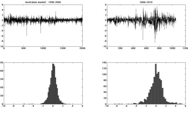
pe-riods for β1 in the GJR-GARCH-AL. . . 47 4 Chapter 2: Plots and histograms of the Australian market for both the
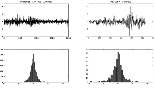
initial learning period and the forecasting period. . . 50 5 Chapter 2: Plots and histograms of the US market for both the initial
learning period and the forecasting period. . . 50 6 Chapter 2: Plots and histograms of the UK market for both the initial
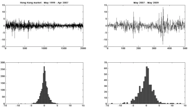
learning period and the forecasting period. . . 51 7 Chapter 2: Plots and histograms of the Hong Kong market for both the
initial learning period and the forecasting period. . . 51 8 Chapter 2: Plots and histograms of the Australian dollar to US dollar for
both the initial learning period and the forecasting period. . . 52 9 Chapter 2: Plots and histograms of the Euro to US dollar for both the
initial learning period and the forecasting period. . . 52 10 Chapter 2: Dynamic shape and skew from GJR-GARCH-AL across six
markets from May 1999 to April 2007. . . 55 11 Chapter 2: Australian stock market: 1-day-ahead 1% VaR forecasts from
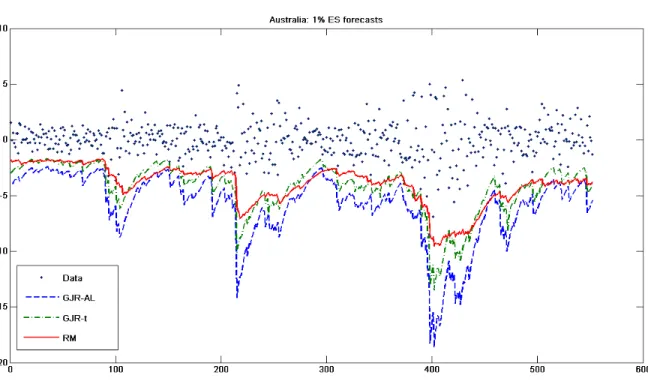
various models. . . 59 12 Chapter 2: Australian stock market: 1% 1-day-ahead ES forecasts from
13 Chapter 2: Forecasts of constant and dynamic shape parameter from the GJR-AL model. . . 80 14 Chapter 2: Dynamic shape estimates from GJR-AL in the Australian
mar-ket from May 1999 to May 2009, plus 95% credible intervals. . . 81 15 Chapter 2: 1% VaR and ES forecast over 10-day horizon from various in
the Australian market. . . 82 16 Chapter 3: Ranges for skewness and kurtosis from TW distribution with
k1 =k2. . . 91 17 Chapter 3: Some standardised two-sided Weibull densities. . . 92 18 Chapter 3: STW, AL, skewed Student t and Student t densities and log
densities. . . 93 19 Chapter 3: MCMC plots in the burn-in period with six different starting
positions forλ1 in the TGARCH-TW model. . . 101 20 Chapter 3: Plots and histograms of the Australian market for both the
initial learning period and the forecasting period. . . 102 21 Chapter 3: Plots and histograms of the US market for both the initial
learning period and the forecasting period. . . 102 22 Chapter 3: Plots and histograms of the UK market for both the initial
learning period and the forecasting period. . . 103 23 Chapter 3: Plots and histograms of the HK market for both the initial
learning period and the forecasting period. . . 103 24 Chapter 3: Plots and histograms of AU/US for both the initial learning
period and the forecasting period. . . 104 25 Chapter 3: Plots and histograms of Euro/US for both the initial learning
period and the forecasting period. . . 104 26 Chapter 3: Plots and histograms of IBM for both the initial learning period
27 Chapter 3: Estimated λ1
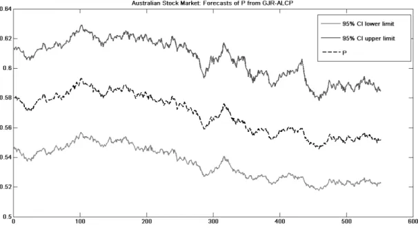
k1 andpfor TGARCH-TW and TGARCH-AL from January 2006 to January 2010. . . 106 28 Chapter 3: 1% VaR forecasts from GJR-n, GJR-t, GJR-skt, GJR-ALCP,
and GJR-TW. . . 109 29 Chapter 3: 1% ES forecasts from GJR-n, GJR-t, GJR-skt, GJR-ALCP,
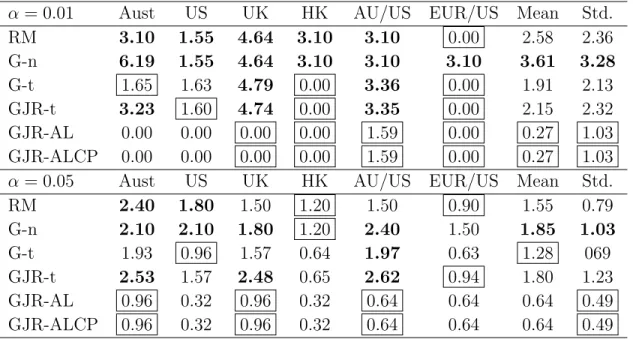
and GJR-TW. . . 111 30 Chapter 3: The ratios of VRate/α at α = 0.01,0.05 for the pre-crisis and
post-crisis periods. . . 115 31 Chapter 3: The ratios of ESRate/δα atα= 0.01,0.05 for the pre-crisis and
post-crisis periods. . . 115 32 Chapter 3: Average loss functions of VaR and ES forecasts from various
distributions across various volatility models. . . 117 33 Chapter 4: SPWAL, TW, and AL densitites and log densities. . . 136 34 Chapter 4: Estimates of the GJR-GARCH-AL parameters using AdMit
and MiG proposals.: 400 replications . . . 141 35 Chapter 4: Simulation study of the GJR-GARCH-PWAL model using AdMit.144 36 Chapter 4: Estimates from 100 replications of the GJR-GARCH-PWAL
model using AdMit. . . 145 37 Chapter 4: Ratios of ˆα/α atα= 0.01,0.05. . . 150 38 Chapter 4: 1% VaR forecasts from AS CAViaR, GJR-t, GJR-AL, and
GJR-PWAL. . . 151 39 Chapter 4: 1% ES forecasts from RiskMetrics, t, AL, and
GJR-PWAL. . . 153 40 Chapter 4: ESRatios ˆδα/δα at α= 0.01,0.05. . . 155
41 Chapter 4: Pre-crisis and post-crisis VRate of ˆα/α at α= 0.01,0.05. . . 158 42 Chapter4: Pre-crisis and post-crisis: ESRates of ˆδα/δα atα= 0.01,0.05. . . 158
43 Chapter 4: Loss function for VaR and ES forecasts. . . 162 44 Chapter 4: Log predictive likelihood for six models across five markets. . . 166 45 Chapter 4: Q-Q plots of residuals from the RiskMetrics and the
GJR-GARCH-n model fitting of the return series of the Australian market. . . . 171 46 Chapter 4: Q-Q plots of residuals from the GARCH-t and the
GJR-GARCH-AL model fitting of the return series of the Australian market. . . 171 47 Chapter 4: Q-Q plots of residuals from the GJR-GARCH-TW and the
GJR-GARCH-PWAL model fitting of the return series of the Australian market. . . 172
List of Tables
1 Chapter 2: Summary statistics for parameter estimates from 400 simulated data sets from the GJR-GARCH-AL model. . . 48 2 Chapter 2: Precision and coverage for parameter estimates from 400 simulated
data sets from the GJR-GARCH-AL model. . . 49 3 Chapter 2: Summary statistics of six return series. . . 53 4 Chapter 2: GJR-GARCH-AL parameter estimates and standard errors (bracketed). 53 5 Chapter 2: Ratios of ˆα/α for 1-day-ahead VaR atα= 0.01,0.05. . . 61 6 Chapter 2: Counts of for 1-day-ahead VaR model rejections, at the 5%
signifi-cance level, at risk levelα= 0.01,0.05. . . 62 7 Chapter 2: Before the financial crisis: ratios of ˆα/α for 1-day-ahead VaR at
α= 0.01,0.05. . . 64 8 Chapter 2: Post-Financial Crisis: ratios of ˆα/α for 1-day-ahead VaR at α =
0.01,0.05. . . 65 9 Chapter 2: ES quantile level function for the Gaussian and AL distributions. 66
10 Chapter 2: Nominal levels δα for 1-day-ahead ES for the Gaussian and AL
distributions. . . 67
11 Chapter 2: Estimated nominal ES levelsδα for 1-day-ahead ES atα= 0.01,0.05. 67 12 Chapter 2: ESRatios ˆδα/δα for 1-day-ahead ES atα= 0.01,0.05. . . 67
13 Chapter 2: Counts of 1-day-ahead ES model rejections atα = 0.01,0.05. . . 70
14 Chapter 2: Before the financial crisis: ˆδα/δα for 1-day-ahead ES at α= 0.01,0.05. 71 15 Chapter 2: After the financial crisis: ˆδα/δα for 1-day-ahead ES at α= 0.01,0.05. 71 16 Chapter 2: Average daily market risk charge for 1-day-ahead VaR atα= 0.01. . 72
17 Chapter 2: AD mean of violating 1-day-ahead returns atα= 0.01,0.05.. . . 74
18 Chapter 2: AD maximum of violating for 1-day-ahead returns atα= 0.01,0.05. 75 19 Chapter 2: AD mean for 1-day-ahead ES atα= 0.01,0.05. . . 76
20 Chapter 2: Maximum absolute deviation for 1-day-ahead ES atα= 0.01,0.05. . 76
21 Chapter 2: Loss function for 1-day-ahead VaR atα= 0.01,0.05. . . 77
22 Chapter 2: Loss function for 1-day-ahead ES atα= 0.01,0.05. . . 78
23 Chapter 2: Ratios of ˆα/α for 10-day-ahead VaR at α= 0.01,0.05.. . . 84
24 Chapter 2: ESRates for 10-day-ahead ES atα= 0.05. . . 85
25 Summary statistics for parameter estimates from 100 simulated data sets from the TGARCH-TW model. . . 100
26 Chapter 3: Summary statistics of seven return series. . . 107
27 Chapter 3: TGARCH-TW parameter estimates and standard errors (bracketed). 107 28 Chapter 3: Ratios of ˆα/α atα= 0.01,0.05. . . 119
29 Chapter 3: Counts of model rejections for VaR models atα= 0.01,0.05. . . 120
30 Chapter 3: Estimated nominal ES levelsδα atα= 0.01,0.05. . . 121
31 Chapter 3: ESRatios ˆδα/δα atα= 0.01,0.05. . . 122
33 Chapter 3: Before the financial crisis: ratios of ˆα/α atα= 0.01,0.05. . . 124
34 Chapter 3: Before the financial crisis: ˆδα/δα atα= 0.01,0.05. . . 125
35 Chapter 3: Post-financial crisis: ratios of ˆα/αatα= 0.01,0.05. . . 126
36 Chapter 3: Post-Financial Crisis: Ratios of ˆδα/δα atα= 0.01,0.05. . . 127
37 Chapter 3: Loss function for VaR atα= 0.01,0.05. . . 128
38 Chapter 3: Loss function for ES atα= 0.01,0.05. . . 129
39 Chapter 4: Summary statistics for parameter estimates from 400 simulated data sets from the GJR-GARCH-AL model. . . 142
40 Chapter 4: Summary statistics for parameter estimates from 100 simulated data sets from the GJR-GARCH-PWAL model.. . . 143
41 Chapter 4: Summary statistics of five return series. . . 147
42 Chapter 4: GJR-GARCH-SPWAL parameter estimates and standard errors (bracketed). . . 148
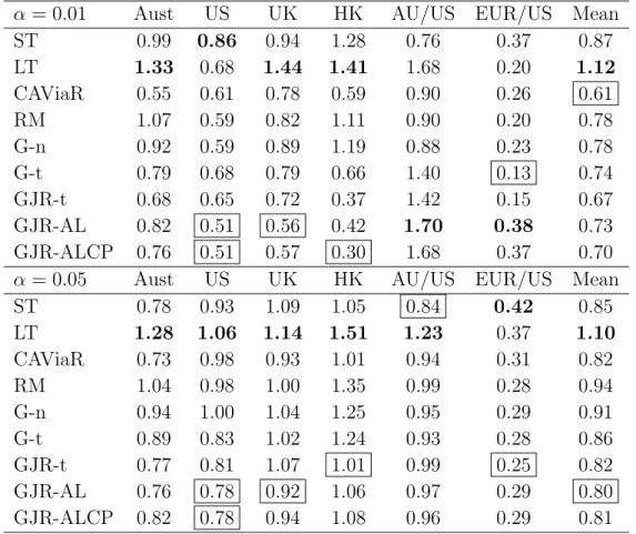
43 Chapter 4: Ratios of ˆα/α atα= 0.01,0.05. . . 149
44 Chapter 4: Counts of model rejections, at the 5% significance level, at risk level α= 0.01,0.05. . . 152
45 Chapter 4: Estimated nominal ES levelsδα atα= 0.01,0.05. . . 154
46 Chapter 4: ESRatios ˆδα/δα atα= 0.01,0.05. . . 156
47 Chapter 4: Counts of ES model rejections at α= 0.01,0.05 . . . 156
48 Chapter 4: Before the financial crisis: ratios of VRate/αatα= 0.01,0.05. . . . 159
49 Chapter 4: Before the financial crisis: ˆδα/δα atα= 0.01,0.05. . . 159
50 Chapter 4: Post-financial crisis: ratios of ˆα/αatα= 0.01,0.05. . . 160
51 Chapter 4: Post-financial crisis: ratios of ˆδα/δα atα= 0.01,0.05. . . 160
52 Chapter 4: Loss function for VaR atα= 0.01,0.05. . . 161
54 Chapter 4: Log predictive likelihood . . . 164
55 Chapter 4: Shapiro-Wilk test. . . 167
56 Chapter 4: Lilliefors test.. . . 167
57 Chapter 4: Chi-square goodness-of-fit test.. . . 168
58 Chapter 4: Jacque-Bera test. . . 168
59 Chapter 4: Ljung-Box test on residuals: a lag of 20. . . 169
60 Chapter 4: Ljung-Box test on squared residuals: 20 lags. . . 169
1
Introduction
The recent Global Financial Crisis (GFC) has once again called into question Financial Risk Management (FRM) methods and practice, as noted in Chen, Gerlach, Lin and Lee (2011). Many regulatory changes were introduced to FRM after the major stock-market crash (“Black Monday”) of October 1987. In order to better control the risk and protect financial institutions against large unexpected losses, the group of G-10 coun-tries agreed in 1988 to sponsor and subsequently form the original Basel Capital Accord (http://www.bis.org/publ/bcbsca.htm). However, in the 1990s, the occurrence of fur-ther financial crises (e.g. Orange County, US, lost $1.6 billion in 1994; in 1995 Barings Bank, UK, lost $1.4 billion; the Long-term Capital Management disaster in 1998) spurred regulators and financial institutions to establish a new benchmark for assessing market risks.
While the stock prices (and financial returns in general) cannot be predicted in the short term or long term, it is possible to forecast risk levels given certain scenarios and investment stances (that is, amount of leverage, long versus short the market, investments in derivatives and options, and so forth). With knowledge of a correctly forecasted risk level (given a set of circumstances), financial entities can manage their capital in a manner that enables them to be as prepared for specific levels of risk as possible. Therefore, loss can be reduced during volatile market movements and risk can be hedged to ensure that these institutions remain profitable.
The fundamental task of this thesis is to develop flexible parametric models for the most well-known and popular modern risk measurement methods, the Value-at-Risk (VaR) and the conditional VaR. The study aims to:
1. Estimate and forecast the potential skewness and dynamics in higher moments for conditional return distributions;
2. Accurately forecast the VaR and conditional VaR.
3. Examine the impacts of asymmetry in the volatility and that in the shape of the conditional return distributions on the VaR and conditional VaR forecasting.
4. Derive an easily applicable backtesting method for conditional VaR or expected shortfall.
5. Improve the efficiency and accuracy of Bayesian computational schemes for param-eter estimation and forecasts.
The major contributions of this work are that it has:
1. Proposed a new model with a conditional asymmetric Laplace return distribution, which repeatedly provides conservative VaR and conditional VaR forecasts.
2. Derived the first four moments, the probability density function (pdf), the cumula-tive density function (cdf), inverse cdf, as well as VaR and conditional VaR functions for an asymmetric Laplace distribution.
3. Derived the function to locate the quantile that the conditional VaR lies at for an asymmetric Laplace distribution, given confidence level α.
4. Developed a more general and flexible distribution, a two-sided Weibull for a con-ditional return distribution, which accurately forecasts the financial tail risks. 5. Derived the first four moments, the pdf, cdf, inverse cdf, VaR and conditional VaR
functions, and the ES quantile function for a two-sided Weibull ditribution.
6. Derived the ES function and ES quantile level function for the skewed Student t of Hansen (1994).
7. Addressed the ‘Capital Charge Puzzle’ by accurately forecasting risk levels via a two-sided Weibull distribution.
8. Proposed a partitioned distribution to address the bimodal problem of the two-sided Weibull ditribution, with better model-fitting performance.
9. Designed an easily comprehensible and applicable backtesting method for ES based on the actual quantile that the conditional VaR falls at.
10. Improved the accuracy of parameter estimation and speed of convergence in the Monte Carlo Markov chain, by employing a mixture of Gaussian proposals.
11. Further improved the accuracy and efficiency of Bayesian inference via a mixture of Student t proposals.
12. Found that the tails of the conditional return distribution play a more important role in VaR and ES forecasting than do the GARCH-type volatility specifications. 13. Derived necessary and sufficient conditions for second-order stationarity of the
GJR-GARCH-AL and GJR-GARCH-TW models.
1.1
Financial Risk Measurement Methods
VaR was pioneered in 1993, as a part of the “Weatherstone 4:15pm” daily risk assessment report, in the RiskMetrics model at J.P. Morgan. In 1996, the Basel Committee on Bank Supervision advised commercial banks to determine a minimum regulatory capital, possibly by using an appropriate internal model that calculated VaR thresholds. VaR represents the market risk as one number: the maximum loss expected on an investment over a given time period at specific levels of confidence. Basel II recommends a backtesting procedure for evaluating and comparing VaR models based on the number of observed violations; that is, when actual losses exceed the VaR, in a hold-out sample period. As an important and popular method, the VaR approach is frequently investigated; see Duffie and Pan (1997), Dowd (1998), Jorion (2000), Dempster (2002), Allen (2003), and Holton (2003), among many others.
Although it is widely used by financial institutions, the practicality of using VaR was questioned at least by 1999, when the Bank of International Settlements (BIS) Committee on the Global Financial System pointed out that extreme market movement events “were in the ‘tail’ of [return] distributions, and that VaR models were [thus] useless for measuring and monitoring market risk.” While this statement stood as an ‘extreme’ view, it is true that VaR does not measure the magnitude of loss for violations, illustrated well by Yamai and Yoshiba (2005). Further, Artzner, Delbaen, Eber, and Heath (1999) found that
VaR does not satisfy the sub-additivity property, that is, the sum of the risks of each asset in a portfolio is no greater than the total risk of the portfolio. Therefore VaR is not a ‘coherent’ risk measure. Consequently, the use of VaR can (sometimes) lead to portfolio concentration rather than diversification. Artzner et al. (1997, 1999) proposed an alternative, coherent measure, called Expected Shortfall (ES) (or conditional VaR, tail VaR, average value at risk, AVaR, or tail conditional expectation, TCE), which gives the expected loss (magnitude) conditional on exceeding a VaR threshold. However, VaR is recommended in Basel II, while ES is not (yet). Hence, both risk measures are considered here.
Basel II recommends a backtesting procedure for evaluating and comparing VaR mod-els based on the number of observed violations; that is, when actual losses exceed the VaR, for a hold-out sample period of at least one year. Under-estimation of VaR (and ES) lev-els can result in institutions setting aside insufficient regulatory capital and thus suffering losses leading to insolvency during extreme market movements. Ewerhart (2002) argued that prudent financial institutions tend to hold unnecessary, excessive regulatory capital to ensure their reputation and quality, while Bakshi and Panayotov (2007) called this the “Capital Charge Puzzle”. Intuitively, overstated VaR will lead financial institutions to al-locate excessive amounts of capital, which may be attractive in the market after the most recent global financial crisis. However, as the goals of financial institutions are to meet the regulatory and capital requirements and to maximize profits and attract investors, such capital over-allocation represents an investment opportunity cost. Thus, although regu-lators may prefer smaller violation numbers in case of excessive losses, investors favour models that accurately predict risk, instead of overpredicting or underpredicting it. The goal of this study is to find a model that accurately predicts risk for the period before the recent global financial crisis as well as during and after the crisis.
1.2
Models for Value-at-Risk and Conditional Value-at-Risk
The recent global financial crisis showed that international financial markets are subject at times to quickly changing volatility and risk levels. Therefore, the crisis called into question, once again, risk measurement and risk management practices. With the
in-auguration of Basel III in 2011, fundamental questions are being raised and examined concerning how to measure risk, or even if, its level can be forecast accurately. There are three categories of methods for VaR and ES estimation according to McNeil and Frey (2000, p. 272):
1. Non-parametric historical simulation,
2. Parametric methods with fully specified volatility processes and conditional distri-butions, and
3. Semi-parametric methods based on the Extreme Value Theory (EVT) or quantile regression.
This thesis focuses on the parametric methods of risk forecasting.
In the academic literature, much interest has focused on conditional asset return dis-tributions (which could help forecast financial risk levels accurately if well specified), with particular attention on two aspects: (i) the time-varying nature of the distribution, for example, volatility; and (ii) the shape and form of the standardised conditional distribu-tion itself, for example, Gaussian; Tsay (2010, Chapter 7) provides an extensive list of models and methods on VaR.
1.2.1 Volatility models
Parametric VaR and ES measures rely heavily on volatility estimation, since this aspect is important for financial returns (well-known since at least the publication by Engle, 1982). Substantial literature now exists on the time-varying, persistent, and nonlinear properties of conditional return volatility. One stream of volatility models are the GARCH speci-fications. Five highly popular and well-known volatility models are: the Autoregressive Conditionally Heteroscedastic (ARCH) model of Engle (1982); the Generalised ARCH (GARCH) of Bollerslev (1986); the EGARCH model of Nelson (1991) and the GJR-GARCH (GJR) model of Glosten et al. (1993), both of which capture the well-known asymmetric volatility effect of Black (1976); and finally the RiskMetrics (RM) IGARCH
model developed by J.P. Morgan (1996). McAleer (2005) discussed these models in de-tail. More recently, fully nonlinear GARCH models have been specified, including the Threshold (T)-GARCH of Zakoian (1994); the Double Threshold (DT)-ARCH of Li and Li (1996); the DT-GARCH of Brooks (2001), and the Smooth Transition (ST-)GARCH of Gonzalez-Rivera (1998) and Gerlach and Chen (2008). A more general Dynamic Asym-metry (DA-)GARCH model, allowing for the dynamics in the multi-threshold structure, is proposed by Caporin and McAleer (2006). Many other models have been proposed that are far too numerous to mention.
The other stream of volatility models are the stochastic volatility (SV) models, which is based on a continuous-time stochastic process. Substantial literature exists for the SV model: it was first introduced by Taylor (1986) as an alternative to GARCH volatility models; Ghysels et al. (2002) and Shephard (2005) among many other authors have well reviewed the SV models. The SV model with Studentt errors is widely adopted to model the heavy tails in the return series. However, practical studies found this model still inadequate to capture the heavier than normal tails, consequently Eraker et al. (2003) and Nakajima and Omori (2008) suggested using a jump component in the SV model to account for the tail fatness of returns. For more details of SV-jump model comparisons, refer to Chernov et al. (2003), Raggi and Bordignon (2006).
More recently, realized volatility model, based on high frequency intraday data, be-comes a quite popular observable proxy for the latent volatility. The RV models are subject to various realized volatility measures and assumption on the dynmaics of return mean and volatility. Intraday squared returns are an intuitive realized volatility measure, while Andersen, Bollerslev, Diebold and Labys (2001) proposed to use intraday data as a more accurate proxy for the latent volatility. This non-parametric volatility model can be used to model leverage effect, jump processes and mixed jump diffusions for the return series.
Furthermore, Taylor (1986) suggested the absolute returns is a long memory series, with slow decaying autocorrelation coefficient. However, GARCH model is short memory model based on squared returns. For more studies on the relation of long memory volatility and option pricing, refer to the studies of Bollerslev and Mikkelsen (1996, 1999), Taylor
(2000) and Ohanissian, Russel and Tsay (2003). Bollerslev, Diebold and Labys (2003) built a vector autoregressive model with long distributed lags on realized volatility (RV) model for exchange rates. Fulvio Corsi (2004) developed a Heterogeneous Autoregressive model of the Realized Volatility (HAR-RV) to account for the long memory, tail fatness and self-similarity of volatility.
On the other hand, compared to the popular GARCH model, SV model is difficult to estimate, while the RV models have no specification on the shapes of the conditional return distribution. As the latter is one of the major focus of the thesis, this paper mainly consider the GARCH volatility models. Particularly, IGARCH is able to capture the long memory feature of return volatility, GJR-GARCH is able to model the leverage effect, non-linear GARCH models are able to examine the regime-switching process. The SV, RV and long memory models with focus on big shocks in the volatility will be of interest for future research.
Chapter 2 focuses on three of the most important and often-used models: GARCH, GJR, and RM IGARCH. In Chapter 3, to account for the nonlinearity and asymmetry in the volatility process, four specific GARCH models of the many enumerated above are reviewed: GARCH, GJR-GARCH, T-GARCH, and ST-GARCH. In Chapter 4, since the GJR-GARCH model did as well as, if not better than the other volatility models in Chapter 3, and with focus on the return distributions, the classic GJR-GARCH model again is adopted to specify the volatility process.
1.2.2 The return distributions
Another important aspect for VaR and ES estimation is the shape of the conditional return distribution. There is considerable empirical evidence that daily asset returns are fat-tailed (or leptokurtic) and also mildly negatively skewed, both unconditionally and conditionally, and thus cannot be adequately characterized solely by mean and variance (see for example Poon and Granger, 2003, among many others). Furthermore, during extreme market movement, the commonly-used GARCH model with Gaussian errors, is usually not able to fully capture the fat-tails (Thavaneswaran, Peiris, and Singh, 2008), influencing the proposal of the GARCH model with Student t error model by Bollerslev
(1987). In two papers, Harvey and Siddique (1999, 2000) argued that skewness in returns may be critical in investment decisions; for example, taking all else as constant, risk-averse investors should prefer portfolios that are right-skewed (that is, fewer but larger payoffs) to those that are left-skewed (that is, fewer but larger losses). Sadly, the recent global financial crisis highlights the danger of a left-skewed asset portfolio: one large loss can wipe out all previous gains. Ait-Sahalia and Brandt (2001) pointed out the importance of including skewness in financial decision making. For other reviews on skewness of financial returns, see Kraus and Litzenberger (1976), Friend and Westerfield (1980), Lim (1989), Richardson and Smith (1993), and Chen (2001). Ait-Sahalia and Brandt (2001) stated the difficulty of applying (forecast) skewness into financial practice.
There have been attempts to overcome this difficulty by adopting non-Gaussian distri-butions in finance. Mandelbrot (1963) and Fama (1965) pioneered the use of non-Gaussian distributions in finance, investigating the stable Paretian and power laws, while Mittnik and Ratchev (1989) also considered the Weibull, log-normal (separately for positive and negative returns), and Laplace distributions as unconditional return distributions. Fama (1965) and Barnea and Downes (1973) also considered mixtures of Gaussian ditribution in this context.
Subsequent to the first-generation ARCH and GARCH models, and because the kur-tosis allowed by Gaussian errors does not often fully capture fat tails in returns, Bollerslev (1987) proposed the GARCH with conditional Student t error model; McCulloch (1985) used a simplified ARCH-type structure with a conditional stable distribution, updated to GARCH by Liu and Brorsen (1995); Nelson (1982) employed the generalised exponential as a conditional distribution in his E-GARCH; Vlaar and Palm (1993) used a mixture of Gaussian errors in a GARCH model; and Haas, Mittnik, and Paolella (2009) developed an asymmetric multivariate version.
For the dynamics in the skewness and kurtosis, Hansen (1994) developed a skewed Student t distribution, combining it with a GARCH model, also allowing both condi-tional skewness and kurtosis to change over time. More recently, Zhu and Galbraith (2009) extended the idea of a skewed Student t by using a generalized asymmetric Stu-dent t conditional distribution, with separate parameters in each tail; Li, Villani, and
Kohn (2009) modelled the conditional distribution with a smooth mixture of asymmetric Student t densities.
For other distributions used in financial modelling, Griffin and Steel (2006) and Jensen and Maheu (2010) employed Dirichlet process mixtures, while Aas and Haff (2006) used a generalised hyperbolic conditional return distribution.
Two particular distributions draw our attention for taking the skewness and heavy tails into account. One is the asymmetric Laplace (AL) distribution, first introduced in Hinkley and Revankar (1977) and applied to modelling financial data by Madan and Seneta (1990) and other researchers. The advantage of the AL distribution (ALD) is that, apart from the flexible excess kurtosis and skewness properties, dynamics in these higher moments can be allowed via a time-varying shape parameter, as proposed in Lu, Huang, and Gerlach (2010), who employed an exponential smoothing procedure and frequentist methods for that purpose. While Lu et al. (2010) considered an exponential smoothed conditional standard deviation model driven by absolute returns, we favour a more con-ventional GJR-GARCH model, driven by squared returns, but with AL errors; this model borrows existing specifications and combines them into a somewhat new Bayesian model. Unlike in Lu et al. (2010), under a Bayesian framework, simultaneous inference for all model parameters is possible; besides, valid finite sample inference can be obtained un-der parameter constraints required for the usual stationarity and positivity conditions of GARCH models; parameter uncertainty can also be accounted for in all forecast distri-butions. The empirical study shows that this model performs well for the time periods before, during, and after the recent global financial crisis, for VaR and ES forecasting, in comparison with a range of popular and often-used risk models/methods. Furthermore, the proposed model is the only one that remains conservative in its risk forecasts during and after the global financial crisis.
Although the regulators may favour this model because it repeatedly over-estimated risk levels and thus was a conservative risk model, especially for the period during the recent global financial crisis, investors may prefer a model that estimates risk levels more accurately. We achieve this by employing a natural and more flexible extension of the Laplace distribution, the Weibull, and subsequently developing a two-sided Weibull (TW)
distribution. After developing this distribution and its properties, we found that Sornette et al. (2000) had developed a symmetric, two-sided modified Weibull, subsequently used in Maleverge and Sornette (2004), as an unconditional distribution for asset returns, in combination with a Gaussian copula, in order to form efficient portfolios; an asymmetric modified Weibull was also briefly discussed.
We propose a slightly more flexible asymmetric TW distribution to use as a condi-tional return distribution in this study. The shape parameters of this TW distribution take value from a wider range, thus allowing more flexible shapes. After employing this more flexible model, we found that the Student t distribution is very accurate for VaR forecasting; however, the two-sided Weibull distribution is at least its equal for VaR fore-casting, and works best for conditional VaR forecasting for the periods before, during, and after the recent global financial crisis.
The TW distribution accurately models the financial tail risks. However, from the empircal study we find the TW with appropriate tails can be potentially bimodal, while it is common knowledge that both the unconditional and conditional distribution of real financial return series are uni-modal. An intuitive and natural solution to this problem is to develop a partitioned distribution with Weibull tails and a uni-modal distribution in the centre. The distribution in the centre can be either symmetric or asymmetric. This partitioned distribution is able to capture the potential skewness and heavy tails in the conditional financial return distribution as well as better to specify the centre.
Several examples have been detailed in the literature of the combination of differ-ent distributions to form a new distribution. Behrens, Lopes, and Gamerman (2004) developed a truncated Gamma with a generalised Pareto distribution in the right tail for estimating the threshold of extreme events. Zhao, Scarrott, Oxley, and Reale (2010) considered a two-stage model, with a GARCH-type model in the first stage, and a nor-mal distribution plus two generalised Pareto distributions in two tails modelling residuals in the second stage. So and Chan (2011) developed a mixture of distributions under a GARCH framework to model the tail asymmetry in financial time series. This mixture of distribution approach partitions the whole conditional distribution into three parts, with a normal distribution and two generalised Pareto distributions for the two tails.
The aforementioned model in So and Chan (2011) is constructed in a manner that is similar to the manner for the partitioned distribution model in this study; namely, both models use distributions from the stable distribution family to capture the heavy tails. Since the conditional distribution of real financial return series has a higher degree of kurtosis (that is, fat tails) than does a normal distribution, we tends to select a more general distribution with a wider range of kurtosis than normal, and with flexibility to be symmetric and asymmetric. Therefore, we choose the asymmetric Laplace distribu-tion, which itself is an example of a partitioned distribudistribu-tion, with one break point and exponential distributions on each side. This is unlike the normal assumption that So and Chan (2011) made for the centre of the distribution.
Finally, very few studies have considered how to test ES models for adequacy or accuracy; see McNeil and Frey (2000). A method is presented in this thesis, based on a suggestion by Kerkhof and Melenberg (2004), using the trait that the ES occurs at specific, constant quantile levels, regardless of the other distribution parameters, for both the Gaussian and AL distribution, depending only on the VaR quantile level α. Thus, for these models the standard tests for correct quantile violation rates and independence can be applied to test for ES violations. Furthermore, we extend the conditional coverage test of Christoffersen (1998), which is a lag 1 test only, to apply as well to multiple lags.
1.3
Bayesian Inference and Forecasting
The Bayesian approach can easily incorporate uncertainty in all unknown factors and for any prior information, thus is a natural choice of inference and forecasting for VaR and ES models. The Bayesian method is widely used to deal with the challenges of capturing various unobservable dynamics and non-linearity, and generating accurate forecasts for the models in all economic activity, including finance. In this thesis, the likelihood functions of most models are of non-standard forms, thus it is difficult to estimate parameters via the Mamixum Likelihood (ML) method. Meanwhile, the moment conditions of the model parameters and the data are difficult to obtain, thus the parameter is unable to be estimated via the Generalized Method of Moments (GMM). Unlike the ML or GMM, Bayesian methods allow simultaneous inference on all parameters in a model, as well as
parameter uncertainty with inclusion of minimum parameter constraints. Therefore, this thesis employs Bayesian methods for parameter inference and forecasting.
1.3.1 Monte Carlo Markov chain for GARCH models
To execute Bayesian methods, the Markov chain Monte Carlo (MCMC) sampling scheme is adopted to sample from the joint posterior density of models and model parameters. A typical Markov chain is constructed by using Metropolis-Hastings (MH) steps with properly chosen proposal distributions. For a certain GARCH-type model, we divide the parameters into two groups, the GARCH parameters and error distribution parameters, and they are sampled in turn as a block in each MCMC iterate. Applications of the MCMC strategy for GARCH models can be found in the work of Muller and Pole (1995), Bauwens and Lubrano (1998), and Vrontos, Dellaportas, and Politis (2000), among many others. Particularly, the griddy Gibbs sampler (GGS) proposed by Bauwens and Lubrano (1998) is able to capture the shape of the posterior by using a comparatively smaller MCMC sample than the classic Gibbs sampler.
This study takes a Bayesian approach for estimation, extending the adaptive MCMC method of Chen and So (2006). We design a novel mixture of Gaussian proposal dis-tributions for the required MH algorithm. Instead of the usual Gaussian random-walk proposal, this proposal will speed up mixing and convergence by reducing the risk of the chain getting stuck in local modes or mixing too slowly. A similar idea was considered by Hoogerheide, Kaashoek, and Van Dijk (2007) using mixtures of Student t proposal distributions targeted to the shape of the posterior. Giordani and Kohn (2008) improved the sampling efficiency by initiating a frequent updating process of the mixture of normal distributions at a very early stage of the chain. Sampling properties are studied and the mixture proposal approach has seen improved results of MCMC estimates. Estimation under the AL distribution in a quantile regression setting has been considered by Yu and Moyeed (2001), and Yu et al. (2003). Meanwhile, Geraci and Bottai (2007) developed MCMC methods in the semi-parametric quantile setting; this setting is different to the parametric case that this thesis primarily considers.
1.4
Methodology for Evaluating the Forecast Performance
1.4.1 Back-text based on violations
Basel II recommends backtesting VaR models to assess forecast accuracy. One of the most commonly used method is the violation rates (VRate), which allow an intuitive evaluation of VaR forecasts. VRate is the proportion of observations whose return exceeds the VaR level (called violations):
VRate = 1 M N+M X t=N+1 I(yt<VaRt) (1)
where n is the in-sample size, M the forecast sample size. If a model correctly specifies the return quantiles, its true VRate should equal the nominal level α. The risk level α is usually chosen as 1% and 5%.
Three formal testing methods are also employed: 1.The unconditional coverage (UC) test of Kupiec (1995): a likelihood ratio (LR) test that VRate = α; 2. The conditional coverage (CC) test of Christoffersen (1998): a joint LR test for independence of viola-tions and UC; 3. The Dynamic Quantile (DQ) test of Engle and Manganelli (2004): an alternative joint test of independence and UC. The DQ test has been found to be more powerful than the lag 1 CC test; see Berkowitz et al. (in press).
As Basel II requires financial institutions reserve capital as insurance to extreme loss of assets, evaluating the size of the reserved capital, is also of interest. The capital set aside is called capital charge or market risk charge, it is set to be the larger of either current estimate of 1% VaR, or the average 1% VaR over the last 60 days multiplied by a penalty factor. The penalty factor is determined by the number of violating returns in the last 250 forecast trading days (approximately the number of trading days in a year). The expected number of losses exceeding 1% VaR in 250 forecast trading days should be 2.5. Banks are punished for using risky models, which have more than 4 violations per year. In this context, the model performance is categorized into three zones as follows:
Mt= 3 , Nviol ≤4 green
3 + 0.2 (Nviol−4) , 5≤Nviol ≤9 yellow
where green indicates good models, yellow indicates less acceptable, and red indicates unacceptable models and requires immediate remedy to improve the risk management. Generally, models with lower MRC are more favoured for the purpose of risk management. Furthermore, McAleer and da Veiga (2008) recommended the absolute deviation (AD) of returns exceeding VaR threshold for comparing the magnitude of loss. Smaller AD values indicate smaller size of loss for violations. However, it is noted that, models can have smaller AD mean and maximum, if they frequently under-estimate risk and end up with large number of violations. Chen, Gerlach, Lin and Lee (2011) pointed out that both the MRC and the AD methods should be combined with violation rates to evaluate the model performance. Thus, models with small MRC or AD is preferable only when they have appropriate violation rates at risk level α. Since the VRate and UC, CC and DQ tests are more effective, MRC and AD tests are only demonstrated in Chapter 2.
Loss functions are also applicable to assess general quantile forecasts. The applicable loss function is the criterion function, minimised in quantile regression estimation, e.g. as in Koenker and Bassett (1978), and can be written as:
LF =
N+M X
t=N+1
(yt−Rt) (α−It). (2)
whereIt is the indicator variable of a violation (i.e. yt < Rt),Rt is the risk forecast, here
we useV aRtfor each model/method. The best risk forecasts in terms of accuracy should
minimise this loss function.
1.4.2 Diagnostic hypothesis tests
It is popular to evaluate the forecasting performance for models, adopting the idea of maximizing the predictive likelihood. The predictive likelihood measures the ability of forecasting (see e.g., Bjornstad, 1990, Davison, 1986 and Butler, 1986 for more details of this forecasting likelihood measure), thus is a suitable measure of fit for out-of-sample forecasts instead of in-sample model fitting. Particularly, Geweke and Keane (2007) and Li, Villani and Kohn (2009) employed predictive likelihood for comparing financial time series models.
hypothesis tests. Smith (1985) first examined several diagnostic tests on nonnormal and non-standard models, whose residuals are not normal. Gerlach, Carter and Kohn (1999) computed the test statistics by using MCMC and importance sampling. For more details of diagnostic methods, that are widely applied to evaluate financial time series models, refer to Diebold, Gunther and Tay (1998) and Diebold, Hahn and Tay (1999).
In Chapter 4, both the forecasting performance and model-fitting performance are the focus of empirical studies. Thus only in Chapter 4, the predictive likelihood and diagnostic tests on the normalized predictive residuals are demonstrated.
1.5
Structure of the Thesis
In Chapter 2, the well-known GJR-GARCH form is used to model the volatility process, capturing the leverage effect; this is accomplished by combining an asymmetric Laplace form as the conditional distribution, accounting for potential skewness and heavy tails in the series. The dynamics at higher moments are specified by the time-varying shape parameter in this distribution. The ES formula is derived for the asymmetric Laplace distribution. A mixture of Gaussian proposal distributions is adopted in the MH algorithm for MCMC samples. The posterior distributions of the unknown parameters are estimated from these samples, hence the estimates of parameters are obtained by summarizing the estimated posterior distributions. The model is applied to forecast VaR and ES for real financial time series. Its performance is compared with popular models from non-parametric, semi-non-parametric, or parametric methods. Models are evaluated in periods before and after the recent global financial crisis, as this is of great interest to the financial community.
In Chapter 3, the scope of the study is expanded to include more general models and methods for VaR and ES. We examine a range of conditional distributions combined with four volatility specifications to forecast the tail risk in real financial return series. Asymmetry in both the volatility process and conditional distributions are considered. Specifically, a TW distribution, of which the AL distribution is a special case, is proposed to model the conditional return distribution. The first four moments, pdf, cdf, inverse cdf
and VaR, as well as the ES and ES quantile functions, are derived for the TW distribution. In the empirical study, one of the findings is that the tails of the conditional return distribution are much more important than the volatility model in VaR and ES forecasting. Furthermore, the TW outperforms other distributions, including the AL distribution, by providing the most accurate risk assessment, both before, during and after the recent global financial crisis.
Chapter 4 addresses the bimodal problem of the TW distribution. A partitioned distribution with Weibull tails and an AL distribution at the centre is proposed, alongside attempts to adequately model the conditional return distribution. The advantage of using Weibull distributions in tails for forecasting tail risk in financial series is proven in Chapter 3. A GJR-GARCH model specifies the volatility process. For parameter estimation, an adaptive MCMC sampling scheme is adopted, employing an MH algorithm with a mixture of Student t proposal distributions. The components of the mixture are determined through the adaptive mixture of the Student t (AdMit) approach of Hoogerheide et al. (2007). In empirical study, the forecasts from the GJR-GARCH-PWAL model, together with a range of competing models, are evaluated via backtesting methods. A number of formal goodness-of-fit tests are employed to evaluate the normalized residuals from the forecasts to evaluate the model fitting. In general, the proposed model ranks second or third in forecasting VaR and ES, closely following the GJR-GARCH-TW model; however, it has the smaller number of rejections than all the other competing models and ranked first in fitting the five series of returns in the empirical study.
Chapter 5 concludes.
1.6
Summary
In a world saturated with information, can quantitative methods make risk forecasting easier? Is there a model to adequately and accurately forecast the risk levels, not being too conservative, yet able to provide acceptable risk coverage? Which component is more important for a parametric VaR model, the correct volatility models, or the correct conditional return distributions?
This thesis addresses the above questions with novel models developed for adequate VaR and ES forecasting. As the goals of financial institutions are to meet the regulatory and capital requirements and in the meantime to maximize profits and attract investors, neither under-estimation of risk nor over-allocation of regulatory capital is desirable. The proposed models include a conservative and two less conservative models, to adapt to various purposes of risk measurements. The conservative model may be favoured for reg-ulatory purposes. The other two models adequately and accurately predicting risk, rather than over-predicting or under-predicting risk; thus they may be favoured by investors due to their accuracy.
This thesis highlights some non-Gaussian distributions, namely asymmetric Laplace (AL), two-sided Weibull (TW), and partitioned distribution of the Weibull and AL (PWAL). These distributions capture the potential skewness and heavy tails in the financial series. The main characteristics of these distributions and their VaR and ES are derived. Vari-ous distributions are assessed under the GARCH frameworks, using both symmetric and asymmetric volatility specifications. As revealed by the empirical study, the correct con-ditional return distribution (or, more specifically, the tails of the distribution), is of prime importance for forecasting the tail risk in financial time series.
2
Bayesian Value-at-Risk and Expected Shortfall
Fore-casting via the Asymmetric Laplace Distribution
The goals of this chapter are to:1. Propose a parametric model for estimating and forecasting financial risk to provide sufficent risk coverage.
2. Capture the potential skewness and heavy tails in the conditional return distribu-tion.
3. Design a backtesting method for ES that can be easily understood and applied. 4. Improve the accuracy of Bayesian inference for parameters and speed up the
cover-gence in the MCMC procedure.
To achieve the above goals, the proposed model in this chapter employs an AL condi-tional return distribution, capturing the potential skewness and heavy tails. By allowing for a time-varying shape parameter for the AL distribution, the dynamics in skewness, kurtosis, and higher moments can be characterised. A classic GJR-GARCH model is used to account for the leverage effect in the volatility process. For parameter estimation and forecast, an adaptive MCMC sampling scheme, employing an MH algorithm with a mixture of Gaussian proposal densities, is adopted to improve the efficiency and accuracy. An ES backtesting method is derived based on the quantile that the ES lies at. The model is applied to produce one-step-ahead and ten-step-ahead VaR and ES forecasts for six return series, covering a two-year period, which includes the global fiancial crisis in 2008. We extended the conditional coverage test of Christoffersen (1998) to allow for more than one lags. Formal and informal tests indicate that the GJR-GARCH-AL model outperformed a number of popular alternative models. The proposed model is the only model providing always conservative risk forecasts before the crisis, as well as during and after the crisis.
The contributions in this chapter are described as follows. First of all, the pdf, cdf, inverse cdf, VaR and ES functions, ES quantile function, and first four moments for the AL
distribution are derived. An ES backtesting method based on the actual ES quantile for level α is easy to understand and to apply for parametric models. Then, AL distribution with a dynamic shape parameter is compared with a constant shape parameter, and empirical evidence shows the assumption of dynamic skewness is necessary. In terms of estimation methodology, simluation studies sees improved estimation performance of MH algorithm with a mixture of Gaussian proposals. Last but not least, evalution of risk forecast performance in different crisis periods is novel as well.
A shortened version of the material in this chapter has been accepted for publication and will appear as Chen, Q., Gerlach, R. and Lu, Z. (2011), “Bayesian Value-at-Risk and expected shortfall forecasting via the asymmetric Laplace distribution,” Computational Statistics & Data Analysis, in press.
2.1
Model Specification
This section reviews the statistical concepts of VaR and ES and addresses the problem of dynamic quantile and conditional expectation estimation via a GARCH-type volatility model with an AL error distribution.
2.1.1 VaR and ES
A general definition of VaR is defined in McNeil, Frey and Embrechts (2005). Given some confidence level α ∈ (0,1), the VaR of the portfolio at the confidence level α is given by the smallest number l such that the probability that the lossL exceedsl is no larger than 1−α. Formally,
VaRα= inf{l ∈ <:P r(L > l)≤1−α}= inf{l∈ <:FL(l)≥α}. (3)
where FL is the cdf of conditional return distribution. Thus, in this term, VaR is a
quantile of loss function.
For a continuous conditional return distribution X, the ES of the portfolio given a lossL with E(|L|)<∞ at confidence level α is defined as:
Therefore, the ES or the conditional VaR can be written as: ESα = 1 α Z α 0 VaRu(FL)du = Z V aRα −∞ xf(x|x < V aRα)dx = Z V aRα −∞ xf(x)/P (x < V aRα)dx = 1 α Z V aRα −∞ xf(x)dx. (4)
There are three main categories of dynamic quantile and ES estimators: (i) non-parametric: where minimal assumptions are made, e.g. sample quantiles (often called historical simulation, HS); (ii) semi-parametric: e.g. quantile regression or the Conditional Autoregressive Value at Risk (CAViaR) model (Engle and Manganelli, 2004); and (iii) fully parametric: which specifies the dynamics and error distribution completely. In the empirical section in this chapter we consider examples from all three categories. However, this section focuses on a proposed parametric model: a GJR-GARCH model with AL distributed errors.
2.1.2 Asymmetric Laplace distribution
Guermat and Harris (2001) used the symmetric Laplace distribution with GARCH volatil-ity to model short-horizon asset returns. Lu et al. (2010) extended this to allow skewness via the ALD. If a random variable X has an ALD, denoted X ∼AL(γ, τ, p), the density function is f(x|γ, τ, p) = bp τ exp " −bp τ |x−γ| 1 pI(x < γ) + 1 1−pI(x > γ) !# , (5) where bp = q
p2+ (1−p)2 and γ, τ and p are location, scale and shape parameters, respectively. This parameterization is different to that in Yu and Zhang (2005, pg. 1867) for improved interpretability. Here, the shape parameter is defined such thatp=P r(X < γ), and γ is the mode. Further, the scale factor bp is included so that Var(X) =τ2.
Volatility models employ i.i.d. error distributions standardized to have mean 0 and variance 1. The standard AL(0,1, p) distribution has density function
f(x|p) =bpexp " −bp|x| 1 pI(x <0) + 1 1−pI(x >0) !# , (6)
where the variance is 1, but the mean is E(X) = 1−b2p
p . Thus Z =X−
1−2p
bp has an ALD,
with shape parameterp, mean 0, and variance 1. This is the proposed error distribution for the GJR-GARCH model. Lu et al. (2010) used the AL in a time-varying parameter standard deviation GARCH model; we slightly simplify and modify their model.
Some other properties of the AL(0,1, p) are
S(X) = 2 ((1−p) 3−p3) b3 p , K(X) = 9(1−p) 4+ 6(1−p)2p2+ 9p4 b4 p ,
where S and K refer to the usual Pearson measures of skewness and kurtosis. Here
p = 0.5 ≡ S(X) = 0 and thus symmetry while p = 0.5 ≡ K(X) = 6. Skewness is a monotonic function of p, ranging from [−2,2] as p ranges from 1 to 0; while kurtosis ranges from 6 to 9, with its maximum at 9 as p→0 or 1. Thus ptunes the shape of the ALD, controlling the skewness, kurtosis, and all higher moments. Specifically, ifp <0.5, the density is skewed to the right; while the opposite applies for p >0.5.
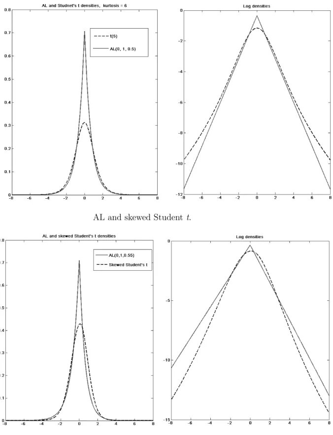
Fat tails or excess kurtosis in conditional financial return distributions are often mod-elled by a Student t distribution. As a comparison, for p = 0.5, both the ALD and standardized Student t distribution with 5 degrees of freedom (DoF) have kurtosis of 6. However, the standardizedt density function is lower than that for an AL(0,1,0.5), from 2 to 6 standard deviations away from the mean. In this region, the symmetric Laplace density has fatter tails. Further, a skewed Student t was proposed by Azzalini and Cap-itanio (2003). For an AL(0,1,0.55), the skewness and kurtosis are approximately −0.4 and 6.2, respectively. A skewed t (α = 0.5, DoF = 5.875) with the same skewness and kurtosis has its left tail heavier than the AL density, between 2 and 6 standard deviations from the mean. In particular,p= 0.55 was a common value found in our empirical studies in Section 5. Figure 1 demonstrates the densities and log densities of AL, Student t, and skewed Student t. The skewed Student t distribution is not considered for conditional return distribution in this Chapter, but is included in Chapter 3 for a more extensive comparison. The tails of the ALD, fatter compared to the Student t distribution, may allow risk measures to be more accurate and effective during a financial crisis.
AL and Student t.
AL and skewed Student t.
obtained directly from (5). Since, in practice, p is usually close to 0.5, while risk man-agement concerns only α levels well away from 0.5, i.e. extreme tails, and thus usually focuses only on the cases α ≤ 0.05. Hence only the case α < p is relevant here; results below are mostly shown only for this case. The AL(0,1, p) cdf is
F(x|p) = Z x −∞ f(u)du = Rx −∞bpexp b pu p du ; x <0 Rx 0 bpexp −bpu 1−p du+R0 −∞bpexp b pu p du ; x≥0 = pexpbpx p ; x <0 p+ (1−p)h1−exp−bpx 1−p i ; x≥0 = pexpbpx p ; x <0 1−(1−p) exp−bpx 1−p ; x≥0. (7) The inverse cdf of the AL(0,1, p) can be easily derived from (7), thus is:
F−1(α|p) = p bp log α p ; 0≤α < p −(1b−p) p log 1−α 1−p ; p≤α <1. (8) The expectation of an AL(0,1, p) for the long position (holding an asset), conditional on being below a quantile level α, is
ESα =
Z V aRα
−∞ xf(x|x < V aRα)dx,
where f(x|x < V aRα) is the conditional density function, which becomes
ESα = Z V aRα −∞ 1 αxbpexp bpx p ! dx = p α " xexp bpx p ! |V aRα −∞ − Z V aRα −∞ exp bpx p ! dx # = p α " V aRαexp bpV aRα p ! − p bp exp bpV aRα p !# .
By substituting the VaRα with the corresponding formula in (8), the ES becomes:
ESα = p α p bp log α p ! − p bp ! bp p p bp log α p !! = p bp " log α p ! −1 # ; 0≤α < p = 1− 1 logαp VaRα ; 0≤α < p. (9)
Similarly, the ES for forAL(0,1, p) for the short position (selling an asset) can be derived and is of the following form:
ESα = − 1−α α 1−p bp " log 1−α 1−p ! −1 # ; p≤α <1 (10) = 1−α α 1− 1 log11−−αp VaRα ; p≤α <1 (11)
2.1.3 GJR-GARCH-ALD model with fixed shape
The GJR-GARCH model is a highly popular volatility model allowing for volatility per-sistence, heavy tails, and the leverage effect of Black (1976). The first model proposed is a GJR-GARCH model with standardised ALD error:
yt = (t−µ)σt (12)
t
i.i.d.
∼ AL(0,1, p)
σt2 = α0+ [α1+α2I(yt−1 <0)]yt2−1+β1σ2t−1.
Here, µ = 1−bp2p and t −µ has mean 0 as standard; the indicator I(·) distinguishes
negative from positive lagged returns. The leverage effect is measured by α2. While the mean return here is fixed at 0, the methods here extend easily to any standard mean equation, such as autoregressions, exogenous regressions, nonlinear models, etc. However, since returns are unpredictable in mean, we chose a mean of 0 here. Sufficient conditions for positivity and stationarity (also necessary) are
α0 >0 ; 0≤α1+β1+α2cp <1
α1, β1, α1+α2 ≥0,
wherecp is derived and given in Appendix 1. The usual value,cp = 0.5, applies only when
p= 0.5, i.e. for symmetry. Using (8) and (9) above, it is straightforward to show that
V aRα,t+1 = σt+1 p bp log α p ! −µσt+1 ESα,t+1 = 1− 1 logαp VaRα,t+1 ; 0≤α < p. (13)
2.1.4 Dynamic higher moments
The recent GFC may induce changes in the process that could be captured by allowing parameters to change dynamically. Since volatility is already heteroscedastic, we choose instead to focus on the higher moments, e.g. skewness and kurtosis. Hansen (1994) proposed a GARCH model with a skewed Student t error distribution, further allowing the skewness and degrees of freedom parameters to be dynamic, as later adopted by Jondeau and Rockinger (2006). Further, Zhu and Galbraith (2009) extended this idea, using a generalized asymmetric Studentt distribution with separate parameters to control skewness and the thickness of each tail.
Instead, we follow Lu et al. (2010), who employed ALD errors and developed a dynamic smoothing equation for the shape parameterp. They showed that the maximum likelihood estimator of p is given by
ˆ p= 1 1 +quv, where u= 1 n X xt>0 |xt| ; v = 1 n X xt<0 |xt|,
with x1, x2, . . . , xn an i.i.d. sample from the AL(0,1, p). A dynamic, exponentially
weighted moving average (EWMA) estimate for each of u and v was proposed as
ut = (1−λ)|xt−1|I(xt−1 >0) +λut−1
vt = (1−λ)|xt−1|I(xt−1 <0) +λvt−1 where 0≤λ ≤1 is the exponential smoothing parameter, and thus
pt= 1 1 +qut vt ; bp[t] = q p2 t + (1−pt)2
was proposed to allow a dynamic shape. This specification, which introduces three extra parameters, namely, the decaying parameter λ, and the initial valuesu0, v0 for u, v, to be estimated, allows all higher moments to change over time, in a manner directly influenced by the standardized data sample x, where from (12) xt=t=yt/σt−µt. u0, v0 are very
2.1.5 GJR-GARCH AL model with dynamic shape
The full model, extended from (12) to allow for dynamic shape, is
yt = (t−µt)σt (14)
t|Ωt−1 ∼AL(0,1, pt)
σ2
t =α0+ (α1+α2I(yt<0))yt2−1+β1σt2−1,
where µt = (1−2pt)/bpt and the previous definitions and restrictions apply. Using (8)
an