Philip John Harding
A thesis submitted for the Degree of
Doctor of Philosophy
University of East Anglia
School of Computing Sciences
July 2013
c
⃝This copy of the thesis has been supplied on condition that anyone who consults it is understood to recognise that its copyright rests with the author and that use of any information derived there from must be in accordance with current UK Copyright Law. In addition, any quotation or extract must include full attribution.
A method of speech enhancement is developed that reconstructs clean speech from a set of acoustic features using a harmonic plus noise model of speech. This is a sig-nificant departure from traditional filtering-based methods of speech enhancement. A major challenge with this approach is to estimate accurately the acoustic features (voicing, fundamental frequency, spectral envelope and phase) from noisy speech. This is achieved using maximum a-posteriori (MAP) estimation methods that oper-ate on the noisy speech. In each case a prior model of the relationship between the noisy speech features and the estimated acoustic feature is required. These models are approximated using speaker-independent GMMs of the clean speech features that are adapted to speaker-dependent models using MAP adaptation and for noise using the Unscented Transform.
Objective results are presented to optimise the proposed system and a set of sub-jective tests compare the approach with traditional enhancement methods. Three-way listening tests examining signal quality, background noise intrusiveness and overall quality show the proposed system to be highly robust to noise, performing significantly better than conventional methods of enhancement in terms of back-ground noise intrusiveness. However, the proposed method is shown to reduce signal quality, with overall quality measured to be roughly equivalent to that of the Wiener filter.
First, thanks go to Dr. Ben Milner for his excellent supervision throughout my time at the University of East Anglia. This work would not have been possible without his support and advice and I owe him a lot for that. I would also like to thank Prof. Stephen Cox for his advice during my PhD as well as his leadership of the Speech, Language and Audio Processing group.
Thanks also go to everyone in the speech lab, past and present, not only for their excellent technical advice, but for making my time at UEA particularly enjoyable. I will miss, and certainly not forget, the time I spent here.
I owe a lot to Connie, as well as my family, and am grateful for all their love and support. Without it I would not have got this far.
Finally, I would also like to acknowledge and thank the UEA and School of Computing Sciences for funding me through my PhD, and also extend my thanks to my examiners, Dr. Barry Theobald and Dr. Mike Brookes, for their comments and suggestions which have no doubt improved the quality of this thesis.
List of Publications vii
List of Abbreviations viii
List of Figures ix List of Tables xx 1 Introduction 1 1.1 Introduction . . . 2 1.1.1 Problem definition . . . 3 1.1.2 Proposed method . . . 4 1.2 Thesis structure . . . 7 1.3 Previous Work . . . 9
2 Speech Enhancement Review 10 2.1 Introduction . . . 11
2.2 Conventional Methods of Speech Enhancement . . . 11
2.2.1 Spectral subtraction . . . 13
2.2.2 Wiener filter . . . 16
2.2.3 Statistical-model-based enhancement . . . 18
2.3 Binary Time-Frequency Masking . . . 23
2.4 Subspace Enhancement . . . 25
2.5 Speech Enhancement by Reconstruction . . . 29
2.6 Measuring Performance . . . 32
2.6.1 Subjective quality measures . . . 32
2.6.2 Objective quality measures . . . 36
2.6.3 Subjective intelligibility measures . . . 40
2.6.4 Objective intelligibility measures . . . 41
2.6.5 Summary . . . 43
3 Speech Reconstruction 44 3.1 Introduction . . . 45
3.2 Speech Production Process . . . 46
3.3 Speech Reconstruction Models . . . 52
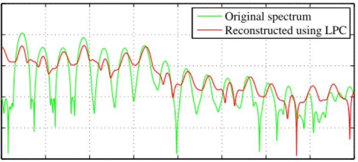
3.3.1 LPC vocoder . . . 52
3.3.2 Sinusoidal model . . . 56
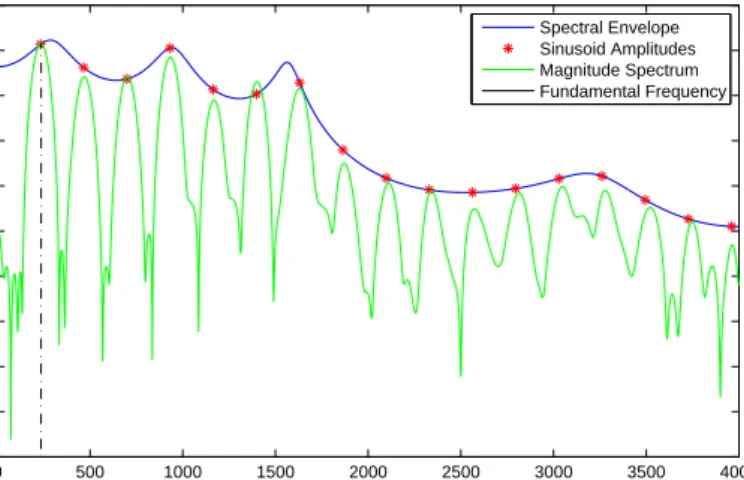
3.3.3 Harmonic plus noise model (HNM) . . . 58
3.3.4 STRAIGHT . . . 65 3.4 Spectral Features . . . 66 3.4.1 Spectrum-based features . . . 67 3.4.2 Filterbank-based features . . . 68 3.4.3 LPC-based features . . . 77 3.5 Results . . . 78
3.5.1 Quality of speech reconstruction . . . 79
3.5.2 Acoustic feature configuration . . . 82
3.5.3 Acoustic feature correlation . . . 86
3.6 Summary . . . 93
4 Methods of Feature Estimation 94 4.1 Introduction . . . 95
4.2 Feature Estimation Review . . . 95
4.2.1 Acoustic feature estimation . . . 96
4.2.2 Feature estimation for robust ASR . . . 97
4.3 Maximuma-posteriori Estimation . . . 100
4.3.1 General definition . . . 101
4.3.2 Gaussian mixture models . . . 102
4.3.3 MAP using Gaussian distributions . . . 104
4.4 Model Training using Stereo Data . . . 108
4.5 Model Adaptation . . . 109
4.5.2 Noise adaptation . . . 114
4.5.3 Adapting for speaker and noise . . . 133
4.6 Summary . . . 134
5 Spectral Envelope Estimation 135 5.1 Introduction . . . 136 5.2 Global Modelling . . . 138 5.3 Localised Modelling . . . 139 5.4 Results . . . 142 5.4.1 Global model . . . 143 5.4.2 Localised models . . . 155 5.4.3 Non-Gaussian noise . . . 165 5.5 Summary . . . 169
6 Fundamental Frequency Estimation 171 6.1 Introduction . . . 172
6.2 F0 Estimation Review . . . 173
6.2.1 Conventional methods of f0 estimation . . . 173
6.2.2 Model-basedf0 estimation . . . 176
6.3 Proposed Method of f0 Estimation . . . 177
6.4 Results . . . 181
6.4.1 Parameter optimisation . . . 182
6.4.2 Estimation from clean speech . . . 183
6.4.3 Estimation from noisy speech . . . 184
6.5 Summary . . . 202
7 Voicing Classification 203 7.1 Introduction . . . 204
7.2 Data-Driven Voicing Classification . . . 205
7.2.1 Classifiers . . . 206
7.2.2 Results . . . 209
7.3 Proposed Method of Voicing Classification . . . 216
7.3.1 Model adaptation . . . 217
7.4 Results . . . 219
7.4.1 Parameter optimisation . . . 219
7.4.2 Voicing classification results . . . 221
7.4.3 Overall results . . . 232
7.5 Summary . . . 233
8 Phase Estimation 235 8.1 Introduction . . . 236
8.2 Phase Models . . . 238
8.2.1 Original signal phase . . . 238
8.2.2 Zero and random phase models . . . 239
8.2.3 Minimum-phase model . . . 241
8.3 Results . . . 243
8.3.1 Objective results . . . 244
8.3.2 Subjective results . . . 259
8.4 Summary . . . 263
9 Speech Enhancement System 264 9.1 Introduction . . . 265
9.2 Speech Enhancement System . . . 265
9.2.1 Proposed method of enhancement . . . 266
9.2.2 Direct inversion . . . 267
9.2.3 Model-based Wiener filter . . . 267
9.3 Results . . . 268
9.3.1 Objective quality measurement . . . 270
9.3.2 Subjective quality measurement . . . 278
9.3.3 Effect of errors in F0 on reconstructed speech quality . . . 286
9.4 Summary . . . 287
10 Conclusions and Further Work 289 10.1 Review . . . 290
10.2 Conclusions . . . 294
10.3 Further Work . . . 295
10.3.2 Acoustic feature estimation . . . 296 A Dataset Descriptions 299 A.1 NuanceCatherine . . . 300 A.2 WSJCAM0 . . . 300 A.3 NOISEX’92 . . . 301 B Phoneme Correlation 303 Bibliography 309
1. Harding, P and Milner, B. (2011). Speech enhancement by reconstruction from cleaned acoustic features. InProceedings of Interspeech, pages 1189-1192 2. Harding, P and Milner, B. (2012). Enhancing Speech by Reconstruction from
Robust Acoustic Features. In Proceedings of Interspeech
3. Harding, P and Milner, B. (2012). On the use of Machine Learning Methods for Speech and Voicing Classification. In Proceedings of Interspeech
ASR Automatic Speech Recognition
CMOS Comparative Mean Opinion Score
DCT Discrete Cosine Transform
f0 Fundamental Frequency
FFT Fast Fourier Transform
GMM Gaussian Mixture Model
HMM Hidden Markov Model
HNM Harmonic plus Noise Model
HTK Hidden Markov Model Toolkit
LFCC Linear-Frequency Cepstral Coefficients
LPC Linear Predictive Coding
LSF Line Spectral Frequencies
MAP Maximum a-posteriori
MFCC Mel-Frequency Cepstral Coefficients
ML Machine Learning
MLLR Maximum Likelihood Linear Regression
MLP Multilayer Perceptron
MOS Mean Opinion Score
OLA Overlap and Add
PCA Principal Component Analysis
PDF Probability Density Function
PMC Parallel Model Combination
SMC Serial Model Combination
SPLICE Stereo-based Piecewise Linear Compensation for Environments STRAIGHT Speech Transformation and Representation using Adaptive
Inter-polation of weiGHTed spectrum
STSA Short-Time Spectral Amplitude
SVM Support Vector Machine
UT Unscented Transform
VAD Voice Activity Detection
VC Voicing Classification
VTS Vector Taylor Series
1.1 Single-channel audio-only speech enhancement . . . 2
1.2 Multi-channel audio-only speech enhancement . . . 3
1.3 Audio-visual speech enhancement . . . 3
1.4 Flowchart of conventional methods of speech enhancement . . . 4
1.5 Narrowband spectrograms showing an utterance in a.) clean condi-tions, b.) white noise at 5dB SNR, c.) babble noise at 5dB SNR, d.) white noise at 5dB SNR and enhanced using log MMSE and e.) babble noise at 5dB SNR and enhanced using log MMSE . . . 5
1.6 Flowchart of speech enhancement methods using speech reconstruc-tion as a post-filter . . . 6
1.7 Flowchart of proposed speech enhancement by reconstruction method 6 2.1 Narrowband spectrograms of utterance “On May evening the rooks were busy building nests in the birch tree”for a) clean speech, b) 10dB car noise and c) after applying spectral subtraction . . . 15
2.2 Level of noise attenuation of maximum likelihood and power spectral subtraction filters in terms of the a-posteriori SNR, γ(k) . . . 19
2.3 Narrowband spectrograms showing: a.) clean speech, b.) noisy speech (white noise at 5dB SNR), c.) the effect of subspace nulling on the noisy speech and d.) the effect of subspace nulling followed by filtering . . . 28
3.1 Illustration of excitation signals in the time and frequency domains, where: a.) voiced excitation signal in the time domain, b.) voiced excitation signal in the frequency domain, c.) unvoiced excitation in the time domain and d.) unvoiced excitation in the frequency domain 47 3.2 Cross section illustrating the human vocal system. Figure adapted from Liesenborgs [2000] . . . 48
3.3 Spectrum illustrating speech formants of voiced phoneme /U/ as spo-ken by a female speaker . . . 49
3.4 Block diagram of the independent source/filter model of speech
pro-duction (Reproduced from Loizou [2007] . . . 50
3.5 Analysis and synthesis processes of the LPC vocoder . . . 53
3.6 Comparison of voiced frames of: a.) original and b.) reconstructed speech using 10th order LPC filter in the time domain . . . 55
3.7 LPC frequency domain response of voiced frame . . . 55
3.8 Comparison of voiced frames of original and reconstructed speech using 10th order LPC filter in the frequency domain . . . 56
3.9 Spectra illustrating the processes of peak picking directly from the magnitude spectrum with a.) no noise and b.) in car noise at 0dB SNR . . . 57
3.10 Spectra illustrating peak picking from the magnitude spectrum using harmonic bands with a.) no noise and b.) car noise at 0dB SNR . . 58
3.11 Spectrum of mixed-excitation frame with voiced/unvoiced transition at approximately 1.6kHz . . . 59
3.12 Illustration of sampling of sinusoid amplitude parameters using spec-tral envelope and estimate of the fundamental frequency . . . 60
3.13 Illustration of step change between harmonic frequencies in periods of rapid f0 change . . . 63
3.14 Narrowband spectrograms of reconstructions of the utterance “and see if it” comparing a.) standard HNM reconstruction and b.) sub-frame reconstruction . . . 63
3.15 Illustration of the overlap and add process in the time domain showing overlapping windows . . . 64
3.16 Reconstructed signal using overlap and add . . . 64
3.17 Flowchart of LFCC/MFCC feature extraction process . . . 69
3.18 Relationship between linear and Mel frequency scales . . . 71
3.19 Visual representation of a.) linear and b.) Mel-spaced filterbank matrices . . . 71
3.20 Flowchart of LFCC/MFCC feature inversion process . . . 74
3.21 Effect of feature inversion on the log-magnitude spectrum with vary-ing number of DCT coefficients retained . . . 76
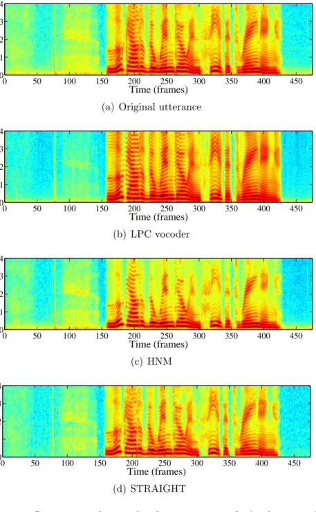
3.22 Comparison of narrowband spectrograms of a.) clean speech and speech reconstructed using: b.) LPC vocoder, c.) HNM and d.) STRAIGHT . . . 80
3.23 Mean LLR of 246 utterances of female speech reconstructed using the HNM using spectral amplitudes estimated from spectral features, LPC, linear-spaced filterbanks and Mel-spaced filterbanks . . . 83
3.24 Mean PESQ of 246 utterances of female speech reconstructed using the HNM using spectral amplitudes estimated from spectral features, LPC, linear-spaced filterbanks and Mel-spaced filterbanks . . . 84 3.25 Effect of discarding DCT coefficients from 32-dimensional MFCC
fea-ture vectors on speech quality as measured using PESQ . . . 85 3.26 Correlation between clean and noisy feature vectors extracted from
30 minutes of female speech using: magnitude spectrum, MFCC and LPC features. . . 87 3.27 Individual feature correlation between clean and noisy MFCCs
ex-tracted from 30 minutes of female speech using white, babble and destroyerops noise at 0dB SNR . . . 88 3.28 Mean overall correlation between MFCC features extracted from noisy
speech andf0 in white, babble and destroyerops noises at varying SNRs 89 3.29 Individual coefficient correlation between f0 and MFCCs with no
noise, white noise and destroyerops noise . . . 91 3.30 Correlation between voicing class and MFCCs in white noise, babble
noise and destroyerops noise at 0dB SNR . . . 92
4.1 Example of using a GMM with 2 mixture components to model the distribution of artificially generated bimodal data . . . 103 4.2 Example of over-fitting and under-fitting distributions using GMM . . 104 4.3 Visual representation of GMM mixture components . . . 105 4.4 Illustration of obtaining the MAP estimate from a single mixture
component (a) and as a weighted average of all mixture components (b)107 4.5 Flowchart illustrating the process of training a joint density model of
clean and noisy speech using stereo training data . . . 109 4.6 Illustration of the process of applying speaker adaptation to a
speaker-independent GMM . . . 110 4.7 Illustration of the process of applying noise adaptation to a GMM of
clean speech . . . 115 4.8 Time domain plots of noise signals comparing: a.) babble noise and
b.) machine gun noise . . . 123 4.9 Distributions of the zero’th MFCC for: a.) babble noise and b.)
machine gun noise . . . 124 4.10 An ergodic hidden Markov model . . . 126 4.11 A circular hidden Markov model . . . 127 4.12 A modified left-right hidden Markov model modelling machine gun
4.13 Noise type detection in machine gun noise using SMC. Spectrograms of a.) clean speech and b.) noisy speech are given for reference. c.) shows the posterior probability of each of the frames belonging to GMMs modelling: i.) low noise, ii.) machine gun recoil and iii.) machine gun burst noise . . . 129 4.14 KL divergence of noise models as a function of the amount of noise
used to train the model for: i.) white noise, ii.) babble noise and iii.) destroyerops noise. . . 133 4.15 Illustration of the process of applying speaker and noise adaptation
to a speaker-independent GMM trained on clean speech . . . 134
5.1 Flowchart illustrating the process of spectral amplitude estimation using a model of the joint density of clean and noisy speech features. 138 5.2 Flowchart illustrating the process of spectral amplitude estimation
using a acoustic-class based models of the joint density of clean and noisy speech features. . . 141 5.3 Effect of varying the number of mixture components on estimated
spectral envelope error measured using LLR . . . 144 5.4 RMS filterbank error of estimated spectral features of a single female
speaker across noise and SNR using speaker-dependent stereo-trained (matched) and noise adapted models in a.) white noise, b.) babble noise and c.) destroyerops noise . . . 146 5.5 LLR of estimated spectral envelope, from a single female speaker,
compared across noise and SNR using speaker-dependent stereo-trained (matched) and noise adapted models in a.) white noise, b.) babble noise and c.) destroyerops noise . . . 148 5.6 RMS filterbank error at 0dB SNR as a function of the amount of noise
used to train the noise models used for adaptation in i.) white noise, ii.) babble noise and iii.) destroyerops noise . . . 148 5.7 Spectral envelope plots of speech enhanced from destroyerops noise
at 5dB SNR using speaker-dependent models adapted with varying amounts of noise data . . . 149 5.8 Effect of varying the amount of data used to train a speaker-dependent
model on estimated filterbank error in white noise at 10dB SNR . . . 150 5.9 Effect of varying the amount of training data used to train speaker
and gender dependent enhancement models on spectral envelope dis-tortion of enhanced speech as measured using LLR in white noise at 10dB SNR . . . 151
5.10 Effect of varying the amount of speaker data used for adaptation when enhancing female speech contaminated with 10dB SNR white noise using a.) speaker-adapted model, b.) speaker-dependent model and c.) gender-dependent model . . . 152 5.11 Performance of using gender-dependent models for clean spectral
en-velope estimation from noisy speech spoken by female speakers mea-sured using LLR . . . 153 5.12 Performance of using gender-dependent models for clean spectral
en-velope estimation from noisy speech spoken by male speakers mea-sured using LLR . . . 154 5.13 Comparison of performance of using speaker-independent models
ver-sus gender-dependent models for the purpose of spectral envelope es-timation from noisy speech contaminated with white noise . . . 155 5.14 Performance of using speaker independent models for clean spectral
envelope estimation from noisy speech spoken by male and female speakers measured using LLR . . . 156 5.15 Spectral envelope RMS error of female speech enhanced using
stereo-trained, speaker-dependent localised models using i.) phoneme classes, ii.) articulation classes in street noise. The use of reference labels (REF) is compared to the obtaining class labels from the HMM-based system (HMM). Performance using a global model is also shown for reference. . . 158 5.16 Two-pass enhancement enhancement system of i.) enhancement using
a global model, before ii.) enhancement using a localised system using global enhanced features as input to the classification system . . . 160 5.17 Phoneme accuracy of female-only phoneme recognition systems trained
on clean speech and tested using i.) noisy speech features, ii.) model adaptation using MLLR, iii.) features compensated for the noise us-ing the proposed system trained on stereo data, and iv.) compensated features and MLLR . . . 161 5.18 Phoneme accuracy of male-only phoneme recognition system using
compensated features and class-based MLLR . . . 162 5.19 Mean LLR of female speech enhanced using the proposed
phoneme-based two-pass enhancement system comparing the use of reference and realistic class labels to the global system . . . 163 5.20 Mean LLR of male speech enhanced using the proposed
phoneme-based two-pass enhancement system comparing the use of reference and realistic class labels to the global system . . . 164
5.21 Performance of SMC enhancement in terms of LLR using speech cor-rupted by machine gun noise at -20dB SNR and enhanced using the global system with SMC noise adaptation applied, displayed as a function of the number of mixture components used to model the noise166 5.22 Spectrograms of an example utterance comparing enhancement using
SMC to conventional methods using speech corrupted by machine gun noise at -20dB SNR . . . 167 5.23 Effect of varying the number of mixture components used for
estima-tion in an SMC-adapted system on the LLR of enhanced speech . . . 169
6.1 Example of autocorrelation analysis in babble noise at 0dB SNR showing clean and noisy speech in a.) the time domain, b.) auto-correlation domain . . . 174 6.2 Illustration of applying stage 3 of the YIN fundamental frequency
estimation algorithm to i.) clean speech and ii.) speech corrupted by babble noise at 0dB SNR . . . 175 6.3 Flowchart of proposed system off0 estimation using model-adaptation
to compensate for speaker and noise . . . 179 6.4 Flowchart of proposed system of f0 estimation using features
com-pensated for speaker and noise using the global enhancement system described in Chapter 5 . . . 180 6.5 Result of varying feature size and number of GMM mixture
com-ponents for the purpose of f0 estimation from MFCCs using MAP estimation in 10dB SNR white noise . . . 182 6.6 Fundamental frequency estimation error (%) using speaker-dependent
models trained on female speech in a.) white noise, b.) babble noise and c.) destroyerops noise . . . 185 6.7 Effect of varying the amount of noise data used to adapt
speaker-dependent models originally trained on clean speech in terms of f0 error (%) across various noises at 0dB SNR . . . 186 6.8 Fundamental frequency estimation error (%) using gender-dependent
models trained on female speech in a.) white noise, b.) babble noise and c.) destroyerops noise . . . 188 6.9 Fundamental frequency estimation error (%) using gender-dependent
models trained on male speech in a.) white noise, b.) babble noise and c.) destroyerops noise . . . 188 6.10 Distributions of referencef0 values used to train a.) speaker-dependent
female model, b.) gender-dependent female model, c.) gender-dependent male model and d.) speaker-independent model . . . 190
6.11 Comparison of performance of gender-dependent system versus speaker-independent system in terms of fundamental frequency error (%) in white noise. . . 191 6.12 Fundamental frequency estimation error (%) using speaker-independent
models in a.) white noise, b.) babble noise and c.) destroyerops noise 192 6.13 Gross fundamental frequency estimation error (%) using
speaker-independent models in a.) white noise, b.) babble noise and c.) destroyerops noise . . . 193 6.14 Comparison of distributions of reference and estimatedf0 values from
speech mixed with babble noise at 0dB SNR where: a.) reference values, b.) estimated using ETSI XAFE system, c.) estimated using YIN and d.) estimated using proposed system using speaker and noise adaptation . . . 194 6.15 Effect of speaker adaptation on distribution of f0 modelled by the
joint density model where a.) compares the unadapted distribution of f0 versus the adapted distribution and b.) shows the distribution of actualf0 values from the target speaker . . . 196 6.16 Comparison of f0 tracks estimated from a single utterance mixed
with babble noise at an SNR of 0dB using a.) YIN, b.) ETSI XAFE and c.) proposed system using noise adaptation . . . 197 6.17 Effect of varying number of mixture components in noise model using
SMC onf0 error in machine gun noise (-20dB SNR) . . . 199 6.18 Time domain example of speech corrupted by machine gun noise at
-20dB SNR . . . 200 6.19 Comparison of f0 tracks estimated from a single utterance mixed
with machine gun noise at an SNR of -20dB using a.) YIN, b.) ETSI XAFE and c.) proposed system using noise adaptation . . . 201
7.1 Performance of voice activity detection in white noise at SNRs of 20dB, 10dB and 0dB in ROC space . . . 211 7.2 Performance of voice activity detection in street noise at SNRs of
20dB, 10dB and 0dB in ROC space . . . 212 7.3 Proposed VC system using model-based speaker and noise
compen-sation . . . 217 7.4 Proposed VC system using compensated features . . . 218 7.5 Effect of varying feature and model sizes on voicing classification error
using models trained and tested on clean speech . . . 220 7.6 Performance of proposed GMM voicing classification system trained
on speaker-dependent data using: i.) clean speech, ii.) noisy speech matched to the testing environment and iii.) model adaptation . . . . 222
7.7 Performance of proposed GMM voicing classification system trained on female-only data using: i.) noisy speech matched to the testing environment, ii.) model adaptation for noise, iii.) model adaptation for speaker and noise and iv.) speaker-dependent system using noise adaptation . . . 224 7.8 Performance of proposed GMM voicing classification system trained
on male-only data using: i.) model adaptation for noise and ii.) model adaptation for speaker and noise . . . 225 7.9 Performance of proposed GMM voicing classification system tested on
female-only data and trained on: i.) gender-independent data using noise adaptation, ii.) gender-independent data using speaker and noise adaptation, iii.) gender-dependent data using environment and noise adaptation and iv.) speaker-dependent data using environment adaptation . . . 226 7.10 Performance of proposed GMM voicing classification system tested
on male-only data and trained on: i.) gender-independent data using noise adaptation, ii.) gender-independent data using speaker and noise adaptation and iii.) gender-dependent data using environment and noise adaptation . . . 228 7.11 Performance of proposed GMM voicing classification system trained
and tested on gender-independent data and compensated for noise using i.) model adaptation, ii.) enhanced features including temporal derivatives and iii.) enhanced features using static coefficients . . . . 230 7.12 Comparison of voicing classification error of best Machine Learning
classifiers trained on clean speech and tested on features extracted from noisy speech and compensated for the noise using the system described in Chapter 5 . . . 231 7.13 Comparison of voicing classification error of the ETSI Aurora XAFE
system and the proposed GMM classification system using i.) en-hanced features and ii.) model adaptation . . . 233
8.1 Diagram of typical analysis/synthesis based speech enhancement system237 8.2 Diagram of phase model in the standard analysis/synthesis framework 237 8.3 Narrowband spectrograms of sinusoids synthesised using zero and
ran-dom phase models using frame widths synchronised and unsynchro-nised with pitch period . . . 240 8.4 Comparison of the overall quality of speech reconstructed using a
8.5 Spectorgrams showing the effect of noisy phase on speech by recon-structing clean speech using the HNM using phase extracted from the same utterance corrupted by destroyerops noise at SNRs of 20dB, 0dB and -20dB . . . 246 8.6 Time-domain plot of sinusoid frames showing no phase error (a) and
an error of eph = π4 (b) for a sinusoid with constant amplitude and
f = 200Hz . . . 247 8.7 Narrowband spectrograms of reconstructed sinusoid signal showing
the effect of phase errors in the frequency domain for a sinusoid with constant amplitude and f = 2kHz. . . 248 8.8 Comparison of narrowband spectrograms of utterance reconstructed
using artificial phase models . . . 250 8.9 Objective quality of speech reconstructed using spectral envelope
es-timated from noisy speech, reference f0 and voicing and a range of phase models . . . 251 8.10 Narrowband spectrograms comparing the effect of using the minimum
phase model with spectral amplitudes estimated from speech at 0dB SNR and reference f0/voicing . . . 252 8.11 Narrowband spectograms illustrating the effect of noisy phase on
speech reconstruction using estimated f0 and clean spectral envelope 254 8.12 Example of incorrectly sampling phase value . . . 255 8.13 Demonstration of the relationship between f0 error and phase error . 256 8.14 Relationship between f0 and (clean) phase errors across a single
ut-terance at 0dB SNR destroyerops . . . 256 8.15 Effect of SNR on average phase error for 1st harmonic of voiced frames257 8.16 Effect of SNR on average phase error for 6th harmonic of voiced frames258 8.17 Objective quality of speech reconstructed using clean spectral
enve-lope, estimatedf0 and voicing and a range of phase models . . . 258 8.18 Objective quality of speech reconstructed using spectral envelope, f0
and voicing estimated from noisy speech and a range of phase models 259 8.19 CMOS results of using estimated spectral envelope and reference f0
(MIN MAP REF). Error bars show confidence intervals at a significance level of p= 0.05. Negative values indicate a preference to the ‘refer-ence’ configuration (first listed). . . 261 8.20 CMOS results of using reference spectral envelope and estimated f0
(MIN REF MAP). Error bars show confidence intervals at a significance level of p = 0.05 Negative values indicate a preference to the ‘refer-ence’ configuration (first listed). . . 262
8.21 CMOS results of using estimated spectral envelope andf0 (MIN MAP MAP). Error bars show confidence intervals at a significance level ofp= 0.05. Negative values indicate a preference to the ‘reference’ configuration
(first listed). . . 263
9.1 Diagram of proposed speech enhancement by reconstruction system . 266 9.2 Objective quality of speech enhancement systems in three noises as measured using PESQ . . . 272
9.3 Comparison of enhancement using HNM (MAP), Wiener (MAP) and Direct (MAP) systems in destroyerops noise at 0dB SNR . . . 273
9.4 Log-spectral frequency response of Wiener (MAP) filter . . . 274
9.5 Comparison of performance of speech enhancement methods in ma-chine gun noise at -20dB SNR . . . 277
9.6 Result of 3-way MOS test measuring signal quality, background noise intrusiveness and overall quality of speech enhancement methods in car noise. Error bars show confidence intervals at a significance level of p= 0.05. . . 280
9.7 Result of 3-way MOS test measuring signal quality, background noise intrusiveness and overall quality of speech enhancement methods in white noise. Error bars show confidence intervals at a significance level of p= 0.05. . . 282
9.8 Result of 3-way MOS test measuring signal quality, background noise intrusiveness and overall quality of speech enhancement methods in babble noise. Error bars show confidence intervals at a significance level of p= 0.05. . . 284
9.9 Result of 3-way MOS test measuring signal quality, background noise intrusiveness and overall quality of speech enhancement methods in machine gun noise. Error bars show confidence intervals at a signifi-cance level of p= 0.05. . . 285
9.10 Effect of modifying f0 in the quality of reconstructed speech as mea-sured using subjective MOS tests and objective PESQ evaluation. Error bars show confidence intervals at a significance level ofp= 0.05 287 A.1 Narrowband spectrogram of noises . . . 302
B.1 Phoneme coefficient feature correlation (affricates) . . . 304
B.2 Phoneme coefficient feature correlation (diphthongs) . . . 304
B.3 Phoneme coefficient feature correlation (fricatives) . . . 305
B.4 Phoneme coefficient feature correlation (liquids) . . . 305
B.6 Phoneme coefficient feature correlation (nasals) . . . 307
B.7 Phoneme coefficient feature correlation (R-coloured vowels) . . . 307
B.8 Phoneme coefficient feature correlation (semi-vowels) . . . 307
B.9 Phoneme coefficient feature correlation (stops) . . . 308
2.1 Comparison Category Rating (CCR) rating scale . . . 33 2.2 Mean Opinion Score (MOS) rating scale . . . 34 2.3 Diagnostic Acceptability Measure (DAM) rating scales . . . 35 2.4 Background intrusiveness rating scale (BAK) . . . 36 2.5 Signal quality rating scale (SIG) . . . 36
3.1 Objective quality, as measured using PESQ and LLR, of 100 utter-ances from different speakers reconstructed using STRAIGHT, LPC vocoder and HNM. . . 79 3.2 Mean phoneme correlation in white noise at 0dB SNR . . . 90
5.1 Speaker-dependent class recognition accuracy (%) in street noise . . . 157 5.2 Phone recognition performance for a speaker-dependent HMM
clas-sification system in clean conditions . . . 160
6.1 Comparison off0 estimation error using proposed system (MAP) and two existing methods of estimation using clean speech . . . 183
7.1 Effect of MFCC feature type on voice activity detection accuracy at an SNR of 10dB in white noise . . . 210 7.2 Voicing classification accuracy in white noise at SNRs of 20dB, 10dB
and 0dB . . . 214 7.3 Voicing classification accuracy in street noise at SNRs of 20dB, 10dB
and 0dB . . . 215
8.1 Minimum-phase test configurations . . . 243
9.1 Objective quality of enhancement systems in the presence of machine gun noise at -20dB SNR . . . 275 9.2 System configurations for first listening test . . . 279
A.1 Voicing class distribution of the NuanceCatherine dataset (Presented in terms of number of 10ms feature vectors) . . . 300 A.2 Voicing class distribution of all male speakers in the WSJCAM0
dataset (Presented in terms of number of 10ms feature vectors) . . . . 301 A.3 Voicing class distribution of all female speakers in the WSJCAM0
dataset (Presented in terms of number of 10ms feature vectors) . . . . 301
Introduction
This chapter describes the problem of speech enhancement and intro-duces the proposed method of speech enhancement by reconstruction. The chapter begins by describing the effect of noise on speech and the constraints on single-channel audio-only speech enhancement. The struc-ture of the thesis is then described.
Contents
1.1 Introduction . . . . 2 1.2 Thesis structure . . . . 7 1.3 Previous Work . . . . 9
Single-channel Speech Enhancement
Figure 1.1: Single-channel audio-only speech enhancement
1.1
Introduction
Speech enhancement is the process of removing the effect of noise from speech recorded in noisy environments. Noise has two main effects on the perception of speech. First, the perceived quality of the signal is deteriorated whilst second, the intelligibility of the speech may also be reduced. The joint effect of these two degra-dations is to increase listener fatigue and, in some cases, to reduce the amount of information which may be successfully conveyed.
In this work a novel method of audio-only single-channel speech enhancement is described. The only available information about the speech is therefore the monau-ral noisy audio signal as illustrated in Figure 1.1. This is a more challenging problem than multi-channel speech enhancement where stereo (or higher dimensional) sig-nals are available which contain sigsig-nals from additional microphones or even video cameras for audio-visual speech enhancement as illustrated in Figures 1.2 and 1.3 re-spectively. In the case of audio-only multichannel speech enhancement the position of the speaker and noise source may be identified to enable better source separa-tion [Meyer and Simmer, 1997], whilst in the case of audio-visual speech enhance-ment facial features such as the position of the lips and other visible articulators, which are not dependent on SNR, may be tracked to provide further information about the speech [Almajai and Milner, 2009]. From this point forward all techniques are described in the context of audio-only single-channel speech enhancement.
Multi-channel Speech Enhancement
Figure 1.2: Multi-channel audio-only speech enhancement
Figure 1.3: Audio-visual speech enhancement
1.1.1
Problem definition
We wish to remove the detrimental effects of the noise whilst preserving the un-derlying speech signal by estimating the clean speech signal, x(m), from the noisy speech, y(m). The noise is assumed to be additive and so the noisy speech signal,
y(m), can be described in terms of the clean signal, x(m), and the noise signal,n(m) as:
y(m) = x(m) +n(m). (1.1)
An intuitive approach to noise remove is therefore to subtract an estimate of the noise from the noisy signal. Noise estimation is inherently challenging, with accurate estimation of the noise impossible. Undesirable effects occur when inac-curate estimates of the noise are subtracted from the noisy signal, and these can be grouped into two categories: underestimation and overestimation. First, in the
Analysis EnhancementAmplitude Synthesis
Conventional Speech Enhancement
Noisy speech Cleaned speech
Figure 1.4: Flowchart of conventional methods of speech enhancement
case of underestimation, some of the noise will remain in the signal after enhance-ment. Second, overestimation of the noise may cause the speech signal to also be suppressed resulting in speech distortion which may further reduce the intelligibility of the speech [Loizou and Kim, 2011].
There are many alternative functions of noise removal, from conventional filtering techniques to binary time-frequency masks and subspace methods. The operation of these methods is illustrated in Figure 1.4 and they are described in more detail in Chapter 2. Whilst these methods have been shown to be effective in relatively low levels of stationary noise, performance reduces in non-stationary noises [Loizou, 2007]. This is largely due to the noise estimation process not accurately tracking the noise and so time varying and impulsive noises often remain in the enhanced signal. The effect of this is shown in Figure 1.5 where log MMSE, one of the best performing methods of speech enhancement, is used to enhance an utterance of female speech with white noise (Figure 1.5(d)) and babble noise (Figure 1.5(e)), both at 5dB SNR. In the case of white noise the noise has been underestimated causing a consider-able amount of residual noise to remain in the signal, similar to the original noise. When the speech is affected by babble noise the enhanced signal contains artifacts known as ‘musical noise’. These artifacts are visible as isolated regions of noise across time and frequency which are audible as annoying ‘musical’ tones and are caused by inaccuracies in noise tracking.
1.1.2
Proposed method
The method of speech enhancement described in this thesis takes an approach of speech enhancement by reconstruction. By reconstructing speech using an
appropri-(a) Clean
(b) White noise (c) Babble noise
(d) White noise (log MMSE) (e) Babble noise (log MMSE)
Figure 1.5: Narrowband spectrograms showing an utterance in a.) clean conditions, b.) white noise at 5dB SNR, c.) babble noise at 5dB SNR, d.) white noise at 5dB SNR and enhanced using log MMSE and e.) babble noise at 5dB SNR and enhanced using log MMSE
Conventional Speech Enhancement Acoustic Feature Extraction Speech Reconstruction Model
Post-filtering using Speech Reconstruction Model
Noisy speech Cleaned speech
Figure 1.6: Flowchart of speech enhancement methods using speech reconstruction as a post-filter Intermediate Feature Extraction Clean Acoustic Feature Estimation Speech Reconstruction Model
Speech Enhancement by Reconstruction
Noisy speech Cleaned speech
Figure 1.7: Flowchart of proposed speech enhancement by reconstruction method
ate model of reconstruction rather than filtering the noisy signal it is expected that artifacts such as musical noise will be eliminated as they will not be reconstructed. The reconstruction model is driven by a set of acoustic features which must be es-timated from the noisy speech. The use of speech reconstruction models in methods of speech enhancement is not a new idea, with several methods having already been developed. These existing methods are described in Chapter 2 and typically extract the acoustic features required for reconstruction from signals that have already been processed by a conventional method of speech enhancement, for example: spectral subtraction, Wiener filtering or log MMSE. This gives a three stage approach of: i.) conventional speech enhancement, ii.) acoustic feature extraction and iii.) speech reconstruction, as illustrated in Figure 1.6.
This work instead aims to estimate the acoustic features required for reconstruc-tion directly from the noisy signal. An intermediate feature for estimareconstruc-tion is first extracted from the noisy speech before the acoustic features required for reconstruc-tion are estimated from this intermediate feature. The proposed system therefore takes a different three stage approach of: i.) noisy feature extraction, ii.) clean acoustic feature estimation and iii.) speech reconstruction (Figure 1.7).
By estimating acoustic features directly from the noisy speech the effect of ar-tifacts caused by conventional methods of estimation should be avoided. This also enables a data-driven approach to acoustic feature estimation.
1.2
Thesis structure
The remainder of this thesis is divided into nine further chapters as follows:
2.) Speech Enhancement Review This chapter describes a number of existing methods of speech enhancement. These include: conventional filtering ap-proaches, subspace methods and binary masking. A number of methods using speech reconstruction models as part of the enhancement process are also de-scribed to put the proposed system in context with existing methods.
3.) Speech Reconstruction Speech reconstruction models that may be used to reconstruct speech for this method of speech enhancement are described in this chapter. All of the considered reconstruction models are driven by a set of acoustic features and so this chapter is split into two parts: first, the recon-struction models are described and second, results from experiments measuring the correlation between the required acoustic features and parameterisations of the noisy speech are reported.
4.) Methods of Feature Estimation This chapter describes a method of acous-tic feature estimation. Maximum a-posteriori (MAP) estimation was chosen for use in this work and relies on a prior model of the joint distribution of the noisy speech and the target acoustic feature. Methods of obtaining these distributions are therefore also described, including methods of speaker and noise adaptation.
5.) Spectral Envelope Estimation Using the method of estimation described in Chapter 4, this chapter describes the proposed system for spectral enve-lope estimation. Two systems are described. First, a method using a global model of speech is described before second, a method using localised models is proposed. The proposed systems are tested against the spectral amplitude estimation component of three conventional methods of speech enhancement: spectral subtraction, Wiener filtering and log MMSE.
6.) Fundamental Frequency Estimation A method of fundamental frequency (f0) estimation using MAP estimation is described in this chapter. Perfor-mance of the proposed system is evaluated in comparison with two conven-tional methods off0 estimation: YIN and ETSI XAFE estimator.
7.) Voicing Classification This chapter describes a method of voicing classifica-tion. The chapter begins by reviewing a range of Machine Learning methods for the purpose of voicing classification to determine the most suitable method of data-driven classification. The most suitable method is then evaluated.
8.) Phase Estimation The final acoustic feature required for reconstruction is phase. This chapter therefore evaluates a range of phase models including: noisy signal phase, zero-phase, random-phase and minimum-phase models. Each model is evaluated in terms of the quality of reconstructed speech mea-sured using both objective and subjective tests.
9.) Speech Enhancement System This chapter describes the proposed method of speech enhancement by reconstruction. The optimal speech reconstruction model as determined in Chapter 3 is driven by the acoustic features estimated using the methods described in Chapters 5-8 to reconstruct cleaned speech. This method is compared to conventional methods of enhancement as well as two more recent methods of reconstruction including a method of direct MFCC inversion and a model-based Wiener filter, constructed using spectral envelope estimated using the method described in Chapter 5. Performance is evaluated objectively using PESQ and subjectively using listening tests.
10.) Conclusions and Further Work The final chapter is split into two sec-tions. The first draws conclusions about the proposed method of speech en-hancement whilst the second describes how the system may be extended.
There are two appendices: Appendix A describes the datasets used in this work whilst Appendix B shows within-class correlation between clean and noisy MFCC feature vectors.
1.3
Previous Work
This thesis extends the work of Shao [2005] and Darch [2008]. Where this work has been extended, it has been appropriately cited. This work differs from the aforementioned work in several ways, including the following:
1. The method of speech reconstruction from MFCC features described by Shao [2005] was applied to the problem of speech enhancement,
2. The acoustic feature estimation techniques used by Darch [2008] were extended to use improved noise adaptation and the use of speaker-adaptation techniques was also introduced,
3. A review of machine learning methods for voicing classification was undertaken and the use of enhanced speech features was examined as an alternative to model adaptation in noisy conditions,
4. A range of phase estimation methods were applied to the reconstruction model to determine the effect of the use of the phase of the noisy speech on the quality of reconstructed speech.
Speech Enhancement Review
The objective of this chapter is to put the proposed method of speech enhancement into perspective by describing existing methods of speech enhancement. First, conventional methods of speech enhancement are discussed. A general framework is described and then a number of related techniques are discussed. These include approaches based on filtering, binary masking and subspace analysis. More recently, speech reconstruc-tion models have been applied for the purpose of speech enhancement. A number of methods of speech enhancement by reconstruction are there-fore also described in this chapter. Finally, a number of methods of measuring the quality and intelligibility of processed speech are then reviewed.
Contents
2.1 Introduction . . . . 11 2.2 Conventional Methods of Speech Enhancement . . . . . 11 2.3 Binary Time-Frequency Masking . . . . 23 2.4 Subspace Enhancement . . . . 25 2.5 Speech Enhancement by Reconstruction . . . . 29 2.6 Measuring Performance . . . . 32
2.1
Introduction
This chapter is split into two parts. The first describes a number of different ap-proaches to speech enhancement with the aim of putting the proposed method of speech enhancement by reconstruction into perspective with existing methods, whilst the second describes methods of measuring the success of enhancement in terms of quality and intelligibility.
First, conventional methods of speech enhancement that filter out an estimate of the noise from the noisy signal are described in Section 2.2. Next, methods using binary time-frequency masks are described in Section 2.3 whilst subspace methods are described in Section 2.4. Finally, existing methods of speech enhancement by reconstruction are described in Section 2.5.
In terms of evaluation of performance, Section 2.6 describes a number subjective and objective tests used to measure the quality and intelligibility of enhanced speech.
2.2
Conventional Methods of Speech Enhancement
Conventional methods of speech enhancement are defined as those that use a filter to remove an estimate of the noise from the noisy speech to give an estimate of the noise-free speech. These methods typically take an approach of analysis followed synthesis. Before synthesis the signal parameters are modified to reduce the effect of noise to give an analysis-enhancement-synthesis approach. These methods typically focus on enhancing spectral amplitudes and so are also known as short-time spectral amplitude (STSA) methods. The three steps of such an approach can be broadly described as follows:
Analysis Utterances are processed on a frame-by-frame basis. Frames are typically 10-30ms in duration and so within each frame the signal may be assumed stationary. Due to limitations of the discrete Fourier transform (DFT) frames are windowed using a Hamming or Hann window. Frames are therefore usually
also overlapped to avoid aliasing in the modulation domain, with an overlap of 75% required to avoid aliasing completely.. Given a frame of noisy speech a window is applied and the DFT taken as:
Y(k) =
N∑−1
m=0
w(m)y(m)e−j2πkmN for 0≤k ≤N −1, (2.1)
where y(m) and w(m) are the mth samples of the noisy speech and window respectively and Y(k) is the kth frequency bin of the complex spectrum con-sisting ofN bins. The absolute of the complex spectrum is then taken to give the magnitude spectrum, |Y(k)|.
Enhancement In the case of STSA methods, enhancement focuses solely on re-moving the effect of noise on spectral amplitudes. The effect of noise on phase is often assumed to be inaudible [Wang and Lim, 1982], whilst the noisy phase has also been shown to be optimal under certain assumptions Loizou [2007]. Clean spectral amplitudes are estimated in some optimal way using an estimate of the noise. If |Y(k)| = f(|X(k)|,|N(k)|) is a function describing the rela-tionship between spectral amplitudes of speech, |X(k)|, and noise, |N(k)|, to give noisy spectral amplitudes,|Y(k)|, then enhancement methods aim to de-rive the inverse of this function. This gives|Xˆ(k)|=f−1(|Y(k)|,|Nˆ(k)|) where
ˆ
|X(k)|is an estimate of the clean spectral amplitudes and|Nˆ(k)|is an estimate of the noise. There are two challenges to such an approach: i.) computing an accurate estimate of the noise and ii.) designing an appropriate function of noise removal. In most cases the function of noise removal is expressed in terms of a gain function (i.e. filter),H(k), wheref(|Yˆ(k)|,|Nˆ(k)) =H(k)|Y(k)|and
H(k) is computed based on the a−priori and a−posteriori SNRs.
Synthesis Speech frames are resynthesised by taking the inverse DFT of the com-plex spectrum. The modified magnitude spectrum is combined with the
orig-inal phase spectrum as:
ˆ
X(k) = |Xˆ(k)|ej∠Y(k), (2.2)
where ∠X(k) is the phase of the original signal. The inverse DFT is then computed to give the estimated waveform:
ˆ x(m) = 1 N N∑−1 k=0 ˆ X(k)ej2πkmN for 0≤m≤N −1. (2.3)
Overlap and add (OLA) may then be used to recombine frames to give an estimate of the clean speech signal, s(m):
s(m) = x(m)wola(R−m) +x(m)wola(2R−m) for 0≤m ≤R−1, (2.4)
where R = N/2 for 50% overlap and wola(m) is the mth sample of the OLA
window.
There are several classes of noise removal function. These include: spectral subtrac-tion, Wiener filtering, statistical-model-based methods and subspace algorithms [Loizou, 2007]. Three methods of conventional enhancement are now considered. First, spec-tral subtraction is described in Section 2.2.1. Next, Wiener filtering is discussed in Section 2.2.2 before statistical-model-based methods are covered in Section 2.2.3.
2.2.1
Spectral subtraction
Spectral subtraction is one the most basic methods of speech enhancement. As-suming additive noise, an estimate of the noise may be subtracted from the noisy speech to give an estimate of the clean speech. This operation is performed in the frequency domain and is typically only applied to the magnitude spectrum. This noise removal process can be implemented by applying a gain function,H(k), to the
magnitude spectrum of the noisy speech:
|Xˆ(k)|=H(k)|Y(k)|, (2.5)
where the response of H(k) is computed from the noisy speech and estimate of the noise as: H(k) = |X(k)| |X(k)|+|N(k)| = |X(k)| |Y(k)| = 1− |N(k)| |Y(k)|. (2.6)
When H(k) is applied to the noisy magnitude spectrum, |Y(k)|, this reduces to a simple subtraction, i.e:
|Xˆ(k)|=f−1
(|Y(k)|,|Nˆ(k)|) =|Y(k)| − |Nˆ(k)|. (2.7) Subtraction may occur in one of several domains, indexed by p, i.e.:
p
√
|Xˆ(k)|= p
√
f−1(|Y(k)|p,|Nˆ(k)|p), (2.8)
wherep= 1 denotes the magnitude spectrum andp= 2 denotes the power spectrum. The resulting estimate of the clean speech spectrum may be negative in cases where the estimate of the noise is greater than the spectrum of the current frame. This is not valid and so half wave rectification can be applied to set negative values to zero, i.e: Xˆ(k)= |Y(k)|2− |Nˆ(k)|2 if |Y(k)|2 >|Nˆ(k)|2 0 else . (2.9)
Whilst this approach will always give a valid magnitude spectrum half-wave recti-fication of the magnitude spectrum exposes random peaks causing artifacts in the reconstructed speech. The position of these peaks will vary frame-by-frame causing random tones to be heard in the enhanced signal. These tones are often known as
(a) Clean (b) Noisy
(c) Spectral Subtraction
Figure 2.1: Narrowband spectrograms of utterance“On May evening the rooks were busy building nests in the birch tree” for a) clean speech, b) 10dB car noise and c) after applying spectral subtraction
‘musical noise’. Figure 2.1 shows spectrograms of clean speech, noisy speech and speech enhanced by spectral subtraction to illustrate the effect of musical noise. Several alternatives to half-wave rectification have been proposed in the literature. One of these alternatives is to spectrally floor any negative spectral bins to a pro-portion of the noise signal estimate [Berouti et al., 1979]. The noise estimate is multiplied by an oversubtraction factor, α, and then subtracted from the noisy power spectrum. Any non-positive bins are then replaced by the noise estimate scaled by the spectral floor parameter, β:
Xˆ(k)2 = |Y(k)|2−α|Nˆ(k)|2 if |Y(k)|2 >(α+β)|Nˆ(k)|2 β|Nˆ(k)|2 else . (2.10)
This has the effect of enhancing high amplitude peaks, usually associated with speech, whilst leaving some noise in lower amplitude regions where the noise is less perceivable. The over-subtraction of the noise is intended to reduce the ampli-tude of broadband peaks leaving just a number of low ampliampli-tude narrowband peaks. These narrowband peaks are then masked by reintroducing a fraction of the noise estimate back on to the spectrum to fill-in the gaps between the remaining
narrow-band peaks. β controls the amount of residual noise and level of musical noise andα
controlling the level of speech distortion. These parameters are typically determined either through experimentation or by forming an MMSE estimate of the optimal pa-rameters [Sim et al., 1998]. Spectral-band or even spectral-bin level optimisation is also possible by calculatingα(k) and β(k) for allk.
Many tests examining both the quality and intelligibility of speech processed by various configurations of spectral subtraction-based methods have been carried out in the literature [Hu and Loizou, 2006; Vary, 1985]. Intelligibility was found to be mostly unaffected when speech enhanced using spectral subtraction was compared against noisy speech, though in some cases intelligibility was found to be slightly reduced. Overall quality and background noise intrusiveness were shown to be im-proved. Whilst the level of background noise can be significantly reduced, speech signal quality is shown to be slightly decreased.
2.2.2
Wiener filter
Wiener filtering is a method of conventional speech enhancement whereby the cleaned magnitude spectrum is derived based on the minimisation of the mean square error (MSE). The noise removal process is implemented as a filtering operation where the cleaned magnitude spectrum is computed as:
|Xˆ(k)|=H(k)|Y(k)|, (2.11)
where H(k) is the kth component of the Wiener filter. Noise is again assumed to be additive and so y(m) = x(m) +d(m) and the relationship between speech and noise in the power spectral domain is assumed to be:
|Y(k)|2 =f(|X(k)|2,|N(k)|2) = |X(k)|2+|N(k)|2. (2.12) The relationship between speech and noise in Equation 2.12 ignores the effect of cross-terms which are assumed to be zero on average. Section 4.5.2.1 examines this
relationship later in this thesis to determine the effect of this assumption. One method of computing the Wiener filter is therefore:
H(k) = |X(k)| 2 |X(k)|2+|N(k)|2 = |X(k)|2 |Y(k)|2 = 1− |N(k)|2 |Y(k)|2. (2.13)
This leads to the noise suppression function:
|Xˆ(k)|=f−1(|Y(k)|,|Nˆ(k)|) = [ 1− | ˆ N(k)|2 |Y(k)|2 ] |Y(k)|. (2.14)
Alternative methods of computing the Wiener filter values include ana-priori SNR based approach where the filter is given as:
H(k) = ξk
ξk+ 1
, (2.15)
where ξk is thea-priori SNR of the kth frequency component and is computed as:
ξk=
|X(k)|2
|N(k)|2. (2.16)
From these equations it is clear that H(k)→1 for frequency components with high SNR, i.e. large values ofξk whilstH(k)→0 for low values of ξk. This is will result
in regions of the signal with high SNR being emphasised whilst those with low SNR are attenuated. The challenge is therefore to compute the values ofξk. Scalart et al.
[1996] proposed a method of a-priori SNR estimation by tracking the noise whilst several alternative methods have previously been proposed including an iterative approach by Lim and Oppenheim [1978] whilst an approach which tracked the noise using HMMs was developed by Ephraim et al. [1989]. More recently, Hadir et al. [2011] proposed the use of a model-based Wiener filter derived from log-Mel feature vectors. The feature vectors were enhanced using MMSE estimation and inverted to compute the filter response. The Mel filterbank used in the feature extraction processed caused the response of the Wiener filter to be smoothed over frequency which resulted in the fine spectral detail of the speech being retained whilst removing
the majority of the noise.
2.2.3
Statistical-model-based enhancement
Statistical-model-based methods of speech enhancement aim to derive the response of a noise suppression filter,H(k), using statistical methods of estimation. There are three methods of statistical estimation commonly applied to this problem. These are: maximum likelihood (ML) estimation, minimum mean-square-error (MMSE) and maximum a-posteriori (MAP). Each of these methods are described in this section in the context of clean spectral amplitude estimation from noisy spectral amplitudes.
2.2.3.1 Maximum likelihood estimation
Maximum-Likelihood estimation is a widely used method of parameter estimation first applied to speech enhancement by McAulay and Malpass [1980]. Given a vector of noisy spectral amplitudes, |Y|, we wish to estimate the most likely value of the clean spectral amplitudes,|X|, that produced |Y|. This is based on the assumption that whilst the relationship between|X|and|Y|is unknown, it is deterministic, i.e. not random. The most likely value of |X| is therefore computed by maximising the likelihood function, i.e.:
|Xˆ|= arg max
|X| f(|Y|;|X|). (2.17)
The maximum value is determined by differentiating the likelihood function and setting the derivative to zero. Assuming Gaussian distributions, this results in:
|Xˆ(k)|= 1 2 [ |Y(k)|+ √ |Y(k)2| − |Nˆ(k)2| ] , (2.18)
where|Nˆ2|is an estimate of the noise in the power spectral domain. This estimator can be expressed in terms of a filter, H(k), whose frequency response is a function
0 5 10 15 −25 −20 −15 −10 −5 0 a-posterioriSNR (dB) 2 0 lo g10 H ( k ) d B
Maximum Likelihood Estimation Power Spectral Subtraction
Figure 2.2: Level of noise attenuation of maximum likelihood and power spectral subtraction filters in terms of thea-posteriori SNR,γ(k)
of the a-posteriori SNR: HM L(k) = 1 2 + 1 2 √ γ(k)−1 γ(k) , (2.19)
where γ(k) is the a-posteriori SNR and is computed as:
γ(k) = |Y(k) 2|
|Nˆ(k)2|. (2.20)
Clean spectral amplitudes may then be estimated by filtering the noisy spectral amplitudes using H(k):
|Xˆ
M L(k)|=HM L(k)|Y(k)|. (2.21)
The response of the filter is now compared to the case of power spectral subtraction as a function of the a-posteriori SNR. The power spectral subtraction filter can be expressed in terms of γ(k) as:
HP S(k) =
γ(k)−1
γ(k) . (2.22)
The response of HP S(k) and HM L(k) is displayed in Figure 2.2. The ML estimator
to speech enhancement. This is attributed to the lack of any prior knowledge of the speech distribution being accounted for in the process of estimation. The following methods both assume knowledge of a-priori distributions and as a result are shown to perform better.
2.2.3.2 Minimum mean square error
A method of estimation which minimises the mean square error (MSE) may be used to estimate the response of H(k). The MMSE (minimum mean-square error) method of speech enhancement is a statistical estimation method that derives the re-sponse of the gain function using non-linear Bayesian estimation techniques. MMSE requires prior knowledge of the probability density functions (pdfs) of the speech and noise, and by taking into account this prior information the accuracy of the estimator is increased over the maximum-likelihood approach. This section begins by first describing the standard MMSE estimator. Second, a technique estimating log-spectral values, the log MMSE estimator, is covered later in the section.
The first stage of MMSE estimation is to form an appropriate expression of the mean-square error (MSE), i.e.:
e=E
[
(|Xˆ(k)| − |X(k)|)2
]
. (2.23)
In the Bayesian approach the expectation is performed with respect to the joint pdf of the clean and noisy magnitude spectra and so the Bayesian MSE,BM SE is defined
as:
BM SE(|Xˆ(k)|) = ∫ ∫
(|Xˆ(k)| − |X(k)|)2f(Y,|X(k)|)dYd|X(k)|. (2.24) This function is minimised by differentiation and so the MMSE estimate of |X(k)|, |Xˆ(k)|, is given as:
|Xˆ(k)|=
∫
where |Xˆ(k)| is shown to depend on every coefficient ofY and the posterior pdf of |X(k)| is given as:
f(|X(k)| |Y(k)) = f(Y(k)| |X(k)|)f(|X(k)|)
f(Y(k)) . (2.26)
By assuming statistical independence between coefficients the Bayesian MSE esti-mator can be simplified to:
|Xˆ(k)|= ∫ xkf(xk|Y(k))dxk = ∫∞ 0∫ xkf(Y(k)|xk)f(xk)dxk ∞ 0 f(Y(k)|xk)f(xk)dxk . (2.27)
Whilst the MMSE estimator may be used to compute estimates of the clean speech magnitude spectrum it has no basis in the human listening process. The human ear has a logarithmic response to sound intensity and so an MMSE approach to estimation of the log-magnitude spectrum was therefore proposed by [Ephraim and Malah, 1985]. In this approach the MSE is defined as:
elog =E [
(log(|Xˆ(k)|)−log(|X(k)|))2
]
(2.28)
and so the log MMSE estimator is:
log(|Xˆ|) = E[log(|X(k)|)|Y(k)] (2.29)
and so the estimate of the clean speech magnitude spectrum,|Xˆ|, is computed as:
|Xˆ|= exp(E[log(|X(k)|)|Y(k)]). (2.30)
The gain function of the log MMSE estimator, H(k) can then be proven to be:
H(k) = ξ(k) ξ(k) + 1exp ( 1 2 ∫ ∞ v(k) e−t t dt ) , (2.31)