Time Varying Noise Estimation for Speech Enhancement and Recognition Using Sequential Monte Carlo Method

Time-Varying Noise Estimation for Speech

Enhancement and Recognition Using

Sequential Monte Carlo Method

Kaisheng Yao

Institute for Neural Computation, University of California, San Diego, 9500 Gilman Drive, La Jolla, CA 92093-0523, USA Email:[email protected]

Te-Won Lee

Institute for Neural Computation, University of California, San Diego, 9500 Gilman Drive, La Jolla, CA 92093-0523, USA Email:[email protected]

Received 4 May 2003; Revised 9 April 2004

We present a method for sequentially estimating time-varying noise parameters. Noise parameters are sequences of time-varying mean vectors representing the noise power in the log-spectral domain. The proposed sequential Monte Carlo method generates a set of particles in compliance with the prior distribution given by clean speech models. The noise parameters in this model evolve according to random walk functions and the model uses extended Kalman filters to update the weight of each particle as a function of observed noisy speech signals, speech model parameters, and the evolved noise parameters in each particle. Finally, the updated noise parameter is obtained by means of minimum mean square error (MMSE) estimation on these particles. For efficient computations, the residual resampling and Metropolis-Hastings smoothing are used. The proposed sequential estimation method is applied to noisy speech recognition and speech enhancement under strongly time-varying noise conditions. In both scenarios, this method outperforms some alternative methods.

Keywords and phrases:sequential Monte Carlo method, speech enhancement, speech recognition, Kalman filter, robust speech recognition.

1. INTRODUCTION

A speech processing system may be required to work in con-ditions where the speech signals are distorted due to back-ground noise. Those distortions can drastically drop the per-formance of automatic speech recognition (ASR) systems, which usually perform well in quiet environments. Similarly, speech-coding systems spend much of their coding capacity encoding additional noise information.

There have been great interests in developing algo-rithms that achieve robustness to those distortions. In gen-eral, the proposed methods can be grouped into two ap-proaches. One approach is based on front-end process-ing of speech signals, for example, speech enhancement. Speech enhancement can be done either in time-domain, for example, in [1, 2], or more widely used, in spectral domain [3, 4, 5, 6, 7]. The objective of speech enhance-ment is to increase signal-to-noise ratio (SNR) of the pro-cessed speech with respect to the observed noisy speech signal.

The second approach is based on statistical models of speech and/or noise. For example, parallel model combina-tion (PMC) [8] adapts speech mean vectors according to the input noise power. In [9], code-dependent cepstral nor-malization (CDCN) modifies speech signals based on prob-abilities from speech models. Since methods in this model-based approach are devised in a principled way, for example, maximum likelihood estimation [9], they usually have bet-ter performances than methods in the first approach, par-ticularly in applications such as noisy speech recognition [10].

Recently, methods have been proposed for speech en-hancement in nonstationary noise. For example, in [11], a method based on sequential Monte Carlo method is ap-plied to estimate time-varying autocorrelation coefficients of speech models for speech enhancement. This algorithm is more advanced in its assumption that autocorrelation coef-ficients of speech models are time varying. In fact, sequen-tial Monte Carlo method is also applied to estimate noise parameters for robust speech recognition in nonstationary noise [12] through a nonlinear model [8], which was re-cently found to be effective for speech enhancement [13] as well.

The purpose of this paper is to present a method based on sequential Monte Carlo for estimation of noise parameter (time-varying mean vector of a noise model) with its appli-cation to speech enhancement and recognition. The method is based on a nonlinear function that models noise effects on speech [8,12,13]. Sequential Monte Carlo method generates particles of parameters (including speech and noise parame-ters) from a prior speech model that has been trained from a clean speech database. These particles approximate posterior distribution of speech and noise parameter sequences given the observed noisy speech sequence. Minimum mean square error (MMSE) estimation of the noise parameter is obtained from these particles. Once the noise parameter has been es-timated, it is used in subtraction-type speech enhancement methods, for example, Wiener filter and perceptual filter,1 and adaptation of speech mean vectors for speech recogni-tion.

The remainder of the paper is organized as follows. The model specification and estimation objectives for the noise parameters are stated inSection 2. InSection 3, the sequen-tial Monte Carlo method is developed to solve the noise pa-rameter estimation problem.Section 4.3demonstrates appli-cation of this method to speech recognition by modifying speech model parameters. Application to speech enhance-ment is shown in Section 4.4. Discussions and conclusions are presented inSection 5.

Notation

Sets are denoted as {·,·}. Vectors and sequences of vec-tors are denoted by uppercased letters. Time index is in the parenthesis of vectors. For example, a sequenceY(1 :T)=

(Y(1) Y(2) · · · Y(T)) consists of vectorY(t) at timet,

where itsith element isyi(t). The distribution of the vector

Y(t) isp(Y(t)). SuperscriptTdenotes transpose.

The symbol X (or x) is exclusively used for original speech andY (ory) is used for noisy speech in testing en-vironments.N(orn) is used to denote noise.

By default, observation (or feature) vectors are in log-spectral domain. Superscripts lin, l,c denote linear spec-tral domain, log-specspec-tral domain, and cepsspec-tral domain. The symbol∗denotes convolution.

1_{A model for frequency masking [14,15] is applied.}

2. PROBLEM DEFINITION

2.1. Model definitions

Consider a clean speech signalx(t) at timetthat is corrupted by additive background noisen(t).2_{In time domain, the} re-ceived speech signaly(t) can be written as

y(t)=x(t) +n(t). (1)

Assume that the speech signalx(t) and noisen(t) are un-correlated. Hence, the power spectrum of the input noisy nal is the summation of the power spectra of clean speech sig-nal and those of the noise. The output at filter bank jcan be described byylin

j (t)=

mb(m)|

L−1

l=0v(l)y(t−l)e−j2πlm/L|2, summing the power spectra of the windowed signal v(t)∗

y(t) with lengthLat each frequencymwith binning weight b(m).v(t) is a window function (usually a Hamming win-dow) andb(m) is a triangle window.3 _{Similarly, we denote} the filter bank output for clean speech signalx(t) and noise n(t) asxlin

j (t) andnlinj (t) forjth filter bank, respectively. They

are related as

ylin

j (t)=xlinj (t) +nlinj (t), (2)

where jis from 1 toJ, andJis the number of filter banks. The filter bank output exhibits a large variance. In order to achieve an accurate statistical model, in some applications, for example, speech recognition, logarithm compression of

ylin

j (t) is used instead. The corresponding compressed power

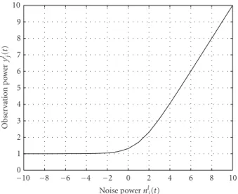
spectrum is called log-spectral power, which has the follow-ing relationship (derived inAppendix A) with noisy signal, clean speech signal, and noise:

yl

j(t)=xlj(t) + log

1 + expnl

j(t)−xlj(t)

. (3)

The function is plotted inFigure 1. We observed that this function is convex and continuous. For noise log-spectral power nl

j(t) that is much smaller than clean speech

log-spectral powerxl

j(t), the function outputsxlj(t). This shows

that the function is not “sensitive” to noise log-spectral power that is much smaller than clean speech log-spectral power.4

We consider the vector for clean speech log-spectral powerXl_(t)=(xl

1(t),. . .,xlJ(t))T. Suppose that the statistics

of the log-spectral power sequenceXl_{(1 :T) can be modeled}

by a hidden Markov model (HMM) with output density at each statest(1≤st≤S) represented by mixtures of Gaussian

M

kt=1πstktN(Xl(t);µ

l stkt,Σ

l

stkt), whereMdenotes the number

2_{Channel distortion and reverberation are not considered in this}

pa-per. In this paper,x(t) can be considered as a speech signal received by a close-talking microphone, andn(t) is the background noise picked up by the microphone.

3_{In Mel-scaled filter bank analysis [16],b(m) is a triangle window}

cen-tered in the Mel scale.

4_{We will discuss later in Sections3.5and4.2that such property may}

10

Figure1: Plot of functionyl

j(t)=xlj(t)+log(1+exp(nlj(t)−xlj(t))). xl

j(t)=1.0;nlj(t) ranges from−10.0 to 10.0.

of Gaussian densities in each state. To model the statistics of noise log-spectral powerNl_{(1 :T), we use a single Gaussian}

density with a time-varying mean vectorµl

n(t) and a constant

diagonal variance matrixVl n.

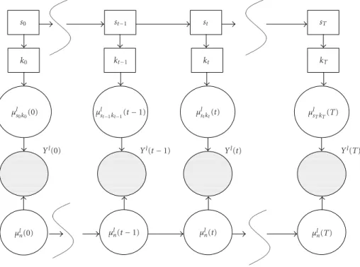
With the above-defined statistical models, we may plot the dependence among their parameters and observation se-quence Yl_{(1 : t) by a graphical model [17] in Figure 2.}

In this figure, the rectangular boxes correspond to discrete state/mixture indexes, and the round circles correspond to continuous-valued vectors. Shaded circles denote observed noisy speech log-spectral power.

The statest ∈ {1,. . .,S}gives the current state index at

framet. State sequence is a Markovian sequence with state transition probabilityp(st|st−1)=ast−1st. At statest, an index

may relate the observed signalYl_{(t) to speech mean vector}

µlstkt(t) and time-varying noise mean vector µ possible modeling error and measurement noise in the above equation.

Furthermore, to model time-varying noise statistics, we assume that the noise parameterµl

n(t) follows a random walk

We collectively denote these parameters {µl

stkt(t),st,kt, ing prior distribution and likelihood at each timet:

pθ(t)|θ(t−1)

Remark 1. In comparison with the traditional HMM, the

new model shown inFigure 2may provide more robustness to contaminating noise, because it includes explicit modeling of the time-varying noise parameters. However, probabilistic inference in the new model can no longer be done by the ef-ficient Viterbi algorithm [18].

2.2. Estimation objective

The objective of this method is to estimate, up to time t, a sequence of noise parameters µl

n(1 : t) given the observed

noisy speech log-spectral sequenceYl_{(1 : t) and the above}

defined graphical model, in which speech models are trained from clean speech signals. Formally,µl

n(1 :t) is calculated by

Based on the graphical model shown in Figure 2, Bayesian estimation of the time-varying noise parameter µl

n(1 : t) involves construction of a likelihood function of

observation sequence Yl_{(1 : t) given parameter sequence}

Θ(1 :t)=(θ(1),. . .,θ(t)) and prior probabilityp(Θ(1 :t)) fort=1,. . .,T. The posterior distribution ofΘ(1 :t) given observation sequenceYl_{(1 :t) is}

pΘ(1 :t)|Yl_{(1 :t)∝pY}l_{(1 :t)|Θ(1 :t)pΘ(1 :t).}

s0 st−1 st sT

k0 kt−1 kt kT

µl

s0k0(0) µ

l

st−1kt−1(t−1) µ

l

stkt(t) µ

l sTkT(T)

Yl_{(0) Y}l_{(t−1) Y}l_{(t) Y}l_(T)

µl

n(0) µln(t−1) µln(t) µln(T)

Figure2: The graphical model representation of the dependence of the speech and noise model parameters.standktdenote the state and Gaussian mixture at frametin speech model.µl

stkt(t) andµ

l

n(t) denote the speech and noise parameters.Yl(t) is the observed noisy speech signal at framet.

Due to the Markovian property shown in (9) and (10), the above posterior distribution can be written as

pΘ(1 :t)|Yl_{(1 :t)}

∝

t

τ=2

pYl_{(τ)|θ(τ)pθ(τ)|θ(τ−1)pY}l_{(1)|θ(1)pθ(1).}

(13) Based on this posterior distribution, MMSE estimation in (11) can be achieved by

ˆ µl

n(1 :t)=

µl 1:n(1:t)

µl

1:n(1 :t)

×

s1:t,k1:t

µl s1:t k1:t(1:t)

pΘ(1 :t)|Yl_{(1 :t)}

dµl

s1:tk1:t(1 :t)dµ

l n(1 :t).

(14)

Note that there are difficulties in evaluating the MMSE estimation. The first relates to the nonlinear function in (10), and the second arises from the unseen state sequence s1:t

and mixture sequencek1:t. These unseen sequences, together

with nodes{µl

stkt(t)},{Y

l_{(t)}, and{µ}l

n(t)}, form loops in the

graphical model. These loops inFigure 2make exact infer-ences on posterior probabilities of unseen sequinfer-encess1:tand

k1:t, computationally intractable. In the following section, we

devise a sequential Monte Carlo method to tackle these prob-lems.

3. SEQUENTIAL MONTE CARLO METHOD FOR NOISE PARAMETER ESTIMATION

This section presents a sequential Monte Carlo method for estimating noise parameters from observed noisy signals and pretrained clean speech models. This method applies se-quential Bayesian importance sampling (BIS) in order to generate particles of speech and noise parameters from a pro-posal distribution. These particles are selected according to their weights calculated with a function of their likelihood. It should be noted that the application here is one particular case of a more general sequential BIS method [19,20].

3.1. Importance sampling

Suppose that there areNparticles{Θ(i)_{(1 :t); i=1,. . .,N}.} Each particle is denoted as

Θ(i)_{(1 :t)=s}(i)

1:t,k1:(i)t,µl_s((ii)) 1:tk

(i) 1:t

(1 :t),µl(i)

n (1 :t)

. (15)

These particles are generated according to p(Θ(1 :t)|Yl_{(1 :}

t)). Then, these particles form an empirical distribution of

Θ(1 :t), given by

¯ pN

Θ(1 :t)|Yl(1 :t)= 1

N

N

i=1

δΘ(i)_(1:t)

dΘ(1 :t), (16)

Using this distribution, an estimate of the parameters of to infinity, this estimate approaches the true estimate under mild conditions [21].

It is common to encounter the situation that the poste-rior distributionp(Θ(1 :t)|Yl_{(1 :t)) cannot be sampled}

di-rectly. Alternatively, importance sampling (IS) method [22] implements the empirical estimate in (17) by sampling from an easier distributionq(Θ(1 : t)|Yl_{(1 : t)), whose support}

Equation (18) can be written as

¯

3.2. Sequential Bayesian importance sampling

Making use of the Markovian property in (13), we can have the following sequential BIS method to approximate the pos-terior distribution p(Θ(1 : t)|Yl_{(1 : t)). Basically, given an}

estimate of the posterior distribution at the previous time t−1, the method updates estimate ofp(Θ(1 :t)|Yl_{(1 :t)) by}

combining a prediction step from a proposal sampling dis-tribution in (24) and (25), and a sampling weight updating step in (26).

Suppose that a sequence of parameters ˆΘ(1 : t−1) up to the previous timet−1 is given. By Markovian property

in (13), the posterior distribution ofΘ(1 :t) =( ˆΘ(1 :t−

We assume that the proposal distribution is in fact given as recursive way; that is,

w(i)(1 :t)= p

Such a time-recursive evaluation of weights can be further simplified by allowing proposal distribution to be the prior distribution of the parameters. In this paper, the proposal distribution is given as

qYl_(t)|θ(i)_{(t)=1, (24)}

Consequently, the above weight is updated by

w(i)_(t)∝w(i)_(t−1)pYl_(t)|θ(i)_(t)pµl(i)

3.3. Rao-Blackwellization and the extended

n (t) is the hidden continuous-valued vector

distributed in N(µln(i)(t); ˆµnl(i)(t−1),Vnl), and Yl(t) is the

observed signal of this model. This integral in (27) can be analytically obtained if we linearize (7) with respect to µln(i)(t). The linearized state-space model provides an

ex-tended Kalman filter (EKF) (see Appendix Bfor the detail of EKF), and the integral isp(Yl_(t)|s(i)

t ,kt(i),µl_s((ii)) t k(ti)(t), ˆµ

l(i)

n (t−

1),Yl_{(t−1)), which is the predictive likelihood shown in}

(B.1). An advantage of updating weight by (27) is its sim-plicity of implementation.

Because the predictive likelihood is obtained from EKF, the weightw(i)_{(t) may not asymptotically approach the target} posterior distribution. One way to achieve asymptotically the target posterior distribution may follow a method called the

extended Kalman particle filter in [26], where the weight is

updated by

However, for the following reasons, we did not apply the stricterextended Kalman particle filterto our problem. First, the scheme in (28) is not Rao-Blackwellized. The variance of sampling weights might be larger than the Rao-Blackwellized method in (27). Second, although observation function (7) is

nonlinear, it is convex and continuous. Therefore, lineariza-tion of (7) with respect toµl

n(t) may not affect the mode

of the posterior distribution p(µl

n(1 : t)|Yl(1 : t)). By the

asymptotic theory (see [25, page 430]), under the mild con-dition that the variance of noise Nl_{(t) (parameterized by}

Vl

n) is finite, bias for estimating ˆµln(t) by MMSE estimation

via (17) with weight given by (27) may be reduced as the number of particlesNgrows large. (However, unbiasedness for estimating ˆµl

n(t) may not be established since there are

zero derivatives with respect to the parameterµl

n(t) in (7).)

Third, evaluation of (28) is computationally more expen-sive than (27), because (28) involves calculation processes on two state-space models. We will show some experiments in

Section 4.1to support the above considerations.

Remark 3. Working in linear spectral domain in (2) for

noise estimation does not require EKF. Thus, if the noise parameter inΘ(t) and the observations are both in the lin-ear spectral domain, the corresponding sequential BIS can achieve asymptotically the target posterior distribution (12). In practice, however, due to the large variance in the lin-ear spectral domain, we may frequently encounter numeri-cal problems that make it difficult to build an accurate sta-tistical model for both clean speech and noise. Compress-ing linear spectral power into log-spectral domain is com-monly used in speech recognition to achieve more accurate models. Furthermore, because the performance by adapting acoustic models (modifying mean and variance of acous-tic models) is usually higher than enhanced noisy speech signals for noisy speech recognition [10], in the context of speech recognition, it is beneficial to devise an algorithm that works in the domain for building acoustic models. In our examples, acoustic models are trained from cepstral or log-spectral features, thus, the parameter estimation algo-rithm is devised in the log-spectral domain, which is lin-early related to the cepstral domain. We will show later that the estimated noise parameter ˆµl

n(t) substitutes ˆµln using a

log-add method (36) to adapt acoustic model mean vec-tors. Thus, to avoid inconsistency due to transformations be-tween different domains, the noise parameter may be esti-mated in log-spectral domain, instead of linear spectral do-main.

3.4. Avoiding degeneracy by resampling

Since the above particles are discrete approximations of the posterior distributionp(Θ(1 :t)|Yl_{(1 :t)), in practice, after}

several steps of sequential BIS, the weights of not all but some particles may become insignificant. This could cause a large variance in the estimate. In addition, it is not necessary to compute particles with insignificant weights. Selection of the particles is thus necessary to reduce the variance and to make efficient use of computational resources.

particles constant, particles with significant weights are du-plicated. The steps are as follows. Firstly, set ˜N(i)_{= Nw˜}(i)_{(1 :}

t). Secondly, select the remaining ¯N=N−N

i=1N˜(i) parti-cles with new weights ´w(i)_{(1 :t)=N}¯−1_{( ˜w}(i)_{(1 :t)N−N}˜(i)_), and obtain particles by sampling in a distribution approx-imated by these new weights. Finally, add the particles to those obtained in the first step. After this residual sampling step, the weight for each particle is 1/N. Besides compu-tational simplicity, residual resampling is known to have smaller variance varN(i) _{= N¯w´}(i)_{(1 : t)(1 −w´}(i)_{(1 : t))} compared to that of SIR (which is varN(i)_{(t) = Nw˜}(i)_{(1 :}

t)(1−w˜(i)_{(1 :t))). We denote the particles after the selection} step as{_Θ˜(i)_{(1 :t); i=1· · ·N}.}

After the selection step, the discrete nature of the approx-imation may lead to large bias/variance, of which the ex-treme case is that all the particles have the same parameters estimated. Therefore, it is necessary to introduce a resam-pling step to avoid such degeneracy. We apply a Metropolis-Hastings smoothing [19] step in each particle by sampling a candidate parameter given the currently estimated param-eter according to the proposal distributionq(θ(t)|_θ˜(i)_(t)). For each particle, a value is calculated as

g(i)(t)=g1(i)(t)g2(i)(t), (30) whereg1(i)(t)=p(( ˜Θ(i)(t−1)θ(t))|Yl(1 :t))/ p( ˜Θ(i)(1 :t)|

Yl_{(1 : t)) and g}(i)

2 (t) = q( ˜θ(i)(t)|θ(t))/q(θ(t)|θ˜(i)(t)). Within an acceptance possibility min{1,g(i)_{(t)}, the Markov} chain then moves towards the new parameterθ(t); other-wise, it remains at the original parameter.

To simplify calculations, we assume that the proposal dis-tributionq(θ(t)|θ˜(i)_{(t)) is symmetric.}5_{Note that p( ˜Θ}(i)_{(1 :}

3.5. Noise parameter estimation via the sequential Monte Carlo method

Following the above considerations, we present the imple-mented algorithm for noise parameter estimation. Given that, at timet−1,Nparticles{_Θˆ(i)_{(1 :t−1); i=1,. . .,N}are}

5_{Generatingθ(t) involves sampling speech states}

t from ˜s(i)1:taccording

to a first-order Markovian transition probabilityp(st|˜s(i)t ) in the graphical

model inFigure 2. Usually, this transition probability matrix is not symmet-ric; that is,p(st|˜s(i)t )=p(˜s(i)t |st). Our assumption of symmetric proposal

distributionq(θ(t)|_θ˜(i)_{(t)) is for simplicity in calculating an acceptance}

possibility.

distributed approximately according top(Θ(1 :t−1)|Yl_{(1 :}

t−1)), the sequential Monte Carlo method proceeds as fol-lows at timet.

Algorithm1.

Bayesian importance sampling step

(1) Sampling. Fori=1,. . .,N, sample a proposal ˆΘ(i)_{(1 :}

ate (B.2)–(B.7) for each particle by EKFs. Predict noise parameter for each particle by

ˆ

where the second term in the right-hand side of the equation is the predictive likelihood, given in (B.1), of the EKF.

(4) Normalization. Fori=1,. . .,N, the weight of theith particle is normalized by

˜

(1) Selection. Use residual resampling to select particles with larger normalized weights and discard those par-ticles with insignificant weights. Duplicate parpar-ticles of large weights in order to keep the number of particles asN. Denote the set of particles after the selection step as{_Θ˜(i)_{(1 :t);i=1,. . .,N}. These particles have equal} weights ˜w(i)_{(1 :t)=1/N.}

Table1: State estimation experiment results. The results show the mean and variance of the mean squared error (MSE) calculated over 100 independent runs.

Algorithm MSE Averaged execution time (s)

Mean Variance

Particle filter 8.713 49.012 5.338

Extended Kalman particle filter 6.496 34.899 13.439

Rao-Blackwellized particle filter 4.559 8.096 6.810

Noise parameter estimation

(1) Noise Parameter Estimation. With the above generated particles at each timet, estimation of the noise param-eterµl

n(t) may be acquired by MMSE. Since each

par-ticle has the same weight, MMSE estimation of ˆµl n(t)

can be easily carried out as

ˆ µl

n(t)=

1 N

N

i=1 ˆ µl(i)

n (t). (35)

The computational complexity of the algorithm at each timetisO(2N) and is roughly equivalent to 2NEKFs. These steps are highly parallel, and if resources permit, can be im-plemented in a parallel way. Since the sampling is based on BIS, the storage required for the calculation does not change over time. Thus the computation is efficient and fast.

Note that the estimated ˆµl

n(t) may be biased from the

true physical mean vector for log-spectral noise powerNl_(t),

because the function plotted inFigure 1has zero derivative with respect tonl

j(t) in regions wherenlj(t) is much smaller

than xlj(t). For those ˆµln(i)(t) which are initialized with

val-ues larger than speech mean vectorµl(i)

s(ti)k( i)

t , updating by EKF may be lower bounded around the speech mean vector. As a result, the updated ˆµl

n(t)=1/N

N

i=1µˆ

l(i)

n (t) may not be the

true noise log-spectral power.

Remark 4. The above problem, however, may not hurt a

model-based noisy speech recognition system, since it is the modified likelihood in (10) that is used to decode speech signals.6_{But in a speech enhancement system, noisy speech} spectrum is directly processed on the estimated noise param-eter. Therefore, biased estimation of the noise parameter may hurt performances more apparently than in a speech recog-nition system.

4. EXPERIMENTS

We first conducted synthetic experiments inSection 4.1to compare three types of particle filters presented in Sections 3.2and3.3. Then, in the following sections, we present ap-plications of the above noise parameter estimation method

6_{The likelihood of the observed signalY}l_{(t), given speech model}

param-eter and a noise paramparam-eter, is the same as long as the noise paramparam-eter is much smaller than the speech parameterµl(i)

s(ti)k(ti) (t).

based on Rao-Blackwellized particle filter (27). We consider particularly difficult tasks for speech processing, speech en-hancement, and noisy speech recognition in nonstationary noisy environments. We show inSection 4.2that the method can track noise dynamically. InSection 4.3, we show that the method improves system robustness to noise in an ASR sys-tem. Finally, we present results on speech enhancement in

Section 4.4, where the estimated noise parameter is used in a

time-varying linear filter to reduce noise power.

4.1. Synthetic experiments

This section7 _{presents some experiments}8 _{to show the} va-lidity of Rao-Blackwellized filter applied to the state-space model in (7) and (8). A sequence ofµl

n(1 :t) was generated

from (8), where state-process noise variance Vl

n was set to

0.75. Speech mean vectorµl

stkt(t) in (7) was set to a constant 10. The observation noise varianceΣl_stkt was set to 0.00005. Given only the noisy observationYl_{(1 : t) fort=1,. . ., 60,}

different filters (particle filter by (26), extended Kalman par-ticle filter by (28), and Rao-Blackwellized particle filter by (27)) were used to estimate the underlying state sequence µl

n(1 : t). The number of particles in each type of filter was

200, and all the filters applied residual resampling [28]. The experiments were repeated for 100 times with random re-initialization ofµl

n(1) for each run.Table 1summarizes the

mean and variance of the MSE of the state estimates, together with the averaged execution time of each filter.Figure 3 com-pares the estimates generated from a single run of the diff er-ent filters. In terms of MSE, the extended Kalman particle filter performed better than the particle filter. However, the execution time of the extended Kalman particle filter was the longest (more than two times longer than that of particle fil-ter (26)). Performance of the Rao-Blackwellized particle fil-ter of (27) is clearly the best in terms of MSE. Notice that its averaged execution time was comparable to that of particle filter.

4.2. Estimation of noise parameter

Experiments were performed on the TI-Digits database downsampled to 16 kHz. Five hundred clean speech utter-ances from 15 speakers and 111 utterutter-ances unseen in the training set were used for training and testing, respectively.

7_{A Matlab implementation of the synthetic experiments is available by}

sending email to the corresponding author.

70

Figure3: Plot of estimates generated by the different filters on the synthetic state estimation experiment versus true state. PF denotes particle filter by (26). PF-EKF denotes particle filter with EKF pro-posal sampling by (28). PF-RB denotes Rao-Blackwellized particle filter by (27).

Digits and silence were respectively modeled by 10-state and 3-state whole-word HMMs with 4 diagonal Gaussian mix-tures in each state.

The window size was 25.0 milliseconds with a 10.0 milliseconds shift. Twenty-six filter banks were used in the binning stage; that is, J = 26. Speech feature vectors were Mel-scaled frequency cepstral coefficients (MFCCs), which were generated by transforming log-spectral power spectra vector with discrete Cosine transform (DCT). The baseline system had 98.7% word accuracy for speech recognition un-der clean conditions.

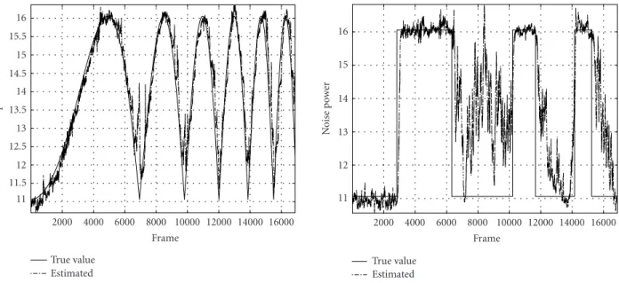
For testing, white noise signal was multiplied by a chirp signal and a rectangular signal in the time domain. The time-varying mean of the noise power as a result changed ei-ther continuously, denoted as experiment A, or dramatically, denoted as experiment B. SNR of the noisy speech ranged from 0 dB to 20.4 dB. We plotted the noise power in the 12th filter bank versus frames inFigure 4, together with the esti-mated noise power by the sequential method with the num-ber of particles N set to 120 and the environment driving noise variance Vl

n set to 0.0001. As a comparison, we also

plotted inFigure 5the noise power and its estimate by the method with the same number of particles but larger driving noise variance set to 0.001.

Four seconds of contaminating noise were used to initial-ize ˆµl

n(0) in the noise estimation method. Initial value ˆµ l(i)

n (0)

of each particle was obtained by sampling fromN( ˆµl n(0) +

ζ(0), 10.0), where ζ(0) was distributed in U(−1.0, 9.0). To apply the estimation algorithm in Section 3.5, observation vectors were transformed into log-spectral domain.

Based on the results in Figures4and5, we make the fol-lowing observations. First, the method can track the evolu-tion of the noise power. Second, the larger driving noise vari-anceVl

n will make faster convergence but larger estimation

error. Third, as discussed inSection 3.5, there was large bias in the region where noise power changed from large to small. Such observation was more explicit in experiment B (noise multiplied with a rectangular signal).

4.3. Noisy speech recognition in time-varying noise The experiment setup was the same as in the previous ex-periments in Section 4.2. Features for speech recognition were MFCCs plus their first- and second-order time diff er-entials. Here, we compared three systems. The first was the baseline trained on clean speech without noise compensa-tion (denoted as Baseline). The second was the system with noise compensation, which transformed clean speech acous-tic models by mapping clean speech mean vectorµl

stktat each statestand Gaussian densityktwith the function [8]

ˆ

n was obtained by averaging noise log-spectral in

noise-alone segments in the testing set. This system was de-noted as stationary noise assumption (SNA). The third sys-tem used the method in Section 3.5to estimate the noise parameter ˆµl

n(t) without training transcript. The estimated

noise parameter was plugged into ˆµl

n in (36) for adapting

acoustic mean vector at each timet. This system was denoted according to the number of particles and variance of the en-vironment driving noiseVl

n.

4.3.1. Results in the simulated nonstationary noise In terms of recognition performance in the simulated non-stationary noise described inSection 4.2,Table 2shows that the method can effectively improve system robustness to the time-varying noise. For example, with 60 particles and the environment driving noise varianceVl

nset to 0.001, the

method improved word accuracy from 75.3%, achieved by SNA, to 94.3% in experiment A. The table also shows that the word accuracies can be improved by increasing the num-ber of particles. For example, given driving noise varianceVl n

set to 0.0001, increasing the number of particles from 60 to 120 could improve word accuracy from 77.1% to 85.8% in experiment B.

4.3.2. Speech recognition in real noise

In this experiment, speech signals were contaminated by highly nonstationary machine gun noise in different SNRs. The number of particles was set to 120, and the environment driving noise varianceVl

nwas set to 0.0001. Recognition

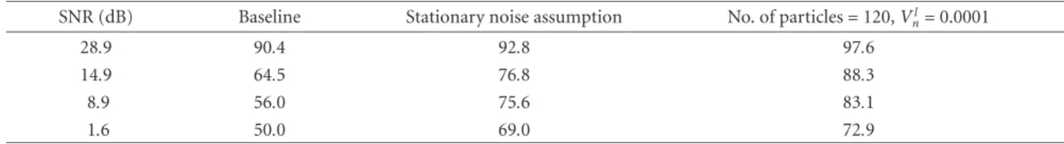
per-formances are shown inTable 3, together with Baseline and SNA. It is observed that, in all SNR conditions, the method in

Section 3.5further improved system performances in

16 15.5 15 14.5 14 13.5 13 12.5 12 11.5 11

No

is

e

p

o

w

er

2000 4000 6000 8000 10000 12000 14000 16000 Frame

True value Estimated

16 15 14 13 12 11

No

is

e

p

o

w

er

2000 4000 6000 8000 10000 12000 14000 16000 Frame

True value Estimated Figure4: Estimation of the time-varying parameterµl

n(t) by the sequential Monte Carlo method at the 12th filter bank in experiment A. The number of particles is 120. The environment driving noise variance is 0.0001. The solid curve is the true noise power, whereas the dash-dotted curve is the estimated noise power.

16 15.5 15 14.5 14 13.5 13 12.5 12 11.5 11

No

is

e

p

o

w

er

2000 4000 6000 8000 10000 12000 14000 16000 Frame

True value Estimated

16 15 14 13 12 11

No

is

e

p

o

w

er

2000 4000 6000 8000 10000 12000 14000 16000 Frame

True value Estimated Figure5: Estimation of the time-varying parameterµl

n(t) by the sequential Monte Carlo method at the 12th filter bank in experiment A. The number of particles is 120. The environment driving noise variance is 0.001. The solid curve is the true noise power, whereas the dash-dotted curve is the estimated noise power.

4.4. Perceptual speech enhancement

Enhanced speech ˆx(t) is obtained by filtering the noisy speech sequencey(t) via a time-varying linear filterh(t); that is,

ˆ

x(t)=h(t)∗y(t). (37)

This process can be studied in the frequency domain as mul-tiplication of the noisy speech power spectrum ylin

j (t) by a

time-varying linear coefficient at each filter bank; that is,

ˆ xlin

j (t)=hj(t)·ylinj (t), (38)

wherehj(t) is the gain at filter bank jat timet. Referring to

(2), we can expand it as

ˆ xlin

j (t)=hj(t)xlinj (t) +hj(t)nlinj (t). (39)

Table2: Word accuracy (%) in simulated nonstationary noise, achieved by the sequential Monte Carlo method in comparison with baseline without noise compensation, denoted as Baseline, and noise compensation assuming stationary noise, denoted as stationary noise assump-tion.

Experiment Baseline

Stationary No. of particles=60 No. of particles=120

noise assumption Vl

n Vnl

0.001 0.0001 0.001 0.0001

A 48.2 75.3 94.3 94.0 94.3 94.6

B 53.0 78.0 82.2 77.1 85.8 85.8

Table3: Word accuracy (%) in machine gun noise, achieved by the sequential Monte Carlo method in comparison with baseline without noise compensation, denoted as Baseline, and noise compensation assuming stationary noise, denoted as stationary noise assumption.

SNR (dB) Baseline Stationary noise assumption No. of particles=120,Vl

n=0.0001

28.9 90.4 92.8 97.6

14.9 64.5 76.8 88.3

8.9 56.0 75.6 83.1

1.6 50.0 69.0 72.9

(1) Wiener filter constructs the coefficient as

hj(t)=1−

ˆ nlin

j (t)

ylin

j (t)

, (40)

where ˆnlinj (t) is the estimate of noise power spectrum.

(2) The criterion for perceptual filter is to constructhj(t)

so that the amplitude of the filtered noise power spec-trahj(t)·nlinj (t) is below the masking threshold of the

denoised speech; that is,

hj(t)·nlinj (t)≤Tj(t), (41)

whereTj(t) is the masking threshold of the denoised

speech signal. The threshold is a function of clean speech spectrumxlinj (t). Sincexlinj (t) is not directly

ob-served, the following equation is used instead, which makes the masking threshold a function of the esti-mated noise power spectra ˆnlin

j (t):

ˆ xlin

j (t)=ylinj (t)−nˆlinj (t). (42)

The perceptual filter exploits the masking properties of the human auditory system, and it has been employed by many researchers (e.g., [14]) in order to provide improved performance over the Wiener filter in low SNR conditions. Masking occurs because the auditory system is incapable of distinguishing two signals close in time or frequency domain. This is manifested by an evaluation of the minimum thresh-old of audibility due to a masker signal. Masking has been widely applied to speech and audio coding [15]. We consider frequency masking [15] when a weak signal is made inaudi-ble by a stronger signal occurring simultaneously.

Both Wiener filter and perceptual filter require the esti-mated noise power spectrum ˆnlin

j (t). Under the assumption

of stationary noise, the noise power spectrum can be esti-mated from noise-alone segments provided by explicit VAD, for example, speech enhancement scheme in [7]. However, in real applications, we encounter time-varying noise, which may change its statistics during speech utterances.

The objective of this section is to test the above de-vised method inSection 3.5for speech enhancement in time-varying noise. The estimated ˆµl

n(t) is converted to linear

spectral domain ˆµlin

n (t) by exponential operation.

Corre-sponding jth element in ˆµlin

n (t) substitutes ˆnlinj (t) in (40)

Log-spectral conversion

Noise parameter estimation

Linear spectral conversion Voice activity

detection

y(t)

Windowing + FFT

Wiener filter Masking threshold calculation

ˆ

x(t)

Filtering Perceptual filter

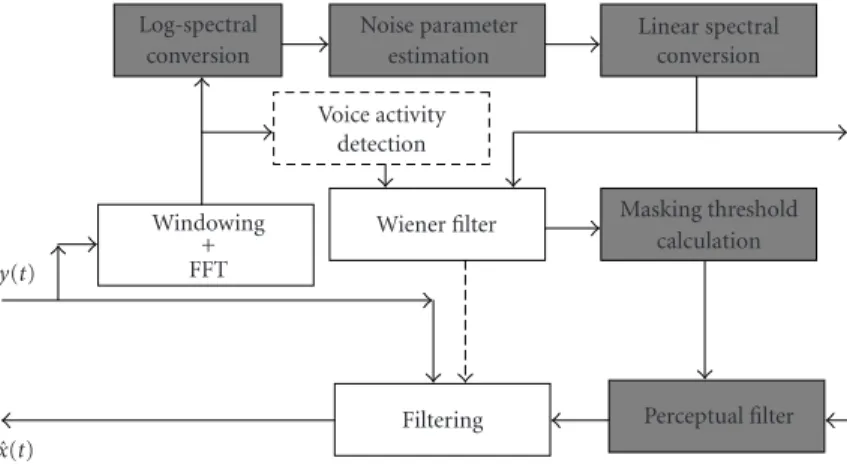
Figure 6: Diagram of the proposed speech enhancement method. Noisy signal y(t) is converted into linear spectral amplitude in “windowing + FFT.” Noise parameter is sequentially estimated in “noise parameter estimation.” The estimated noise parameter is con-verted back into linear spectral domain and is fed into “Wiener filter” to obtain enhanced linear power spectrum. The enhanced spectrum is inputted to “masking threshold calculation,” and the obtained masking threshold is used in perceptual filter with the estimated noise pa-rameter in linear spectral domain. Module “perceptual filter” outputs filter coefficients for speech enhancement in “filtering,” which outputs the enhanced signal ˆx(t).

4.4.1. Masking threshold calculation

The masking thresholdTj(t) is obtained through modeling

the frequency selectivity of the human ear and its masking property. This paper applies a computational model of mask-ing by Johnston [15].

Frequency masking threshold calculation

(1) Frequency analysis. According to a mapping between linear frequency and Bark frequency [14], power spectrum xlinj (t) after short-time Fourier transform (STFT) of input

speech signal is combined in each Bark bankb(1≤b≤B) by

xlin

b (t)= bH

j=bL xlin

j (t), (43)

wherebLandbHdenote the lowest and the highest frequency

for the bark indexb.

(2) Convolution with spreading function. The spreading function Sis used to estimate the effects of masking across critical bands. One example of the spreading functionBbat

b = 2 is plotted inFigure 7. The spread Bark spectrum at bark indexbis denoted asClin

b (t)=Bbxblin(t).

(3) Relative threshold calculation based on tone-like or noise-like determination. The tone-like or noise-like is de-termined by spectral flatness measure (SFM), which is calcu-lated by measuring the decibel (dB) of the ratio of the geo-metric mean of the power spectrum to the arithmetic mean of the power spectrum.

(4) Masking threshold calculation. The relative threshold is subtracted from the spread critical band spectrum to yield the spread threshold estimate.

(5) Renormalization and including absolute threshold information [15].

(6) Converting the masking threshold from Bark fre-quency to linear frefre-quency domain. The masking threshold in linear spectral domainTj(t) is obtained as a result.

−100

−200 −300

−400 −500 −600

Spr

eading

function

(dB)

2 4 6 8 10 12 14 16 18

Critical band number

Figure7: Spreading function for the noise masking threshold cal-culation. The plot shows the spreading function applied to critical band at 2.

An example of masking threshold in linear spectral do-main for a given input spectrum is plotted inFigure 8. The sampling frequency is 8 kHz. Therefore, the total number of critical bands isB=18. In the method presented above, the masking threshold is calculated from the clean speech sig-nal.

4.4.2. Wiener filter and perceptual filter

We apply the method inSection 3.5for time-varying noise parameter estimation. The jth element in ˆµl

n(t) is converted

to linear spectral domain by exponential operation and then substitutes ˆnlin

j (t) in (40) and (42), respectively, for Wiener

20 18 16 14 12 10 8 6 4

A

m

plitude

(dB)

0 500 1000 1500 2000 2500 3000 3500 4000 Frequency (Hz)

Amplitude of speech spectrum Masking threshold

Figure8: Example of the masking thresholdTb(t).

4.4.3. Experimental results

Experiments were performed on Aurora 2 database. Speech models were trained on 8840 clean speech utterances. The model was an HMM with 18 states and 8 Gaussian mix-tures in each state. Noise model was a single Gaussian density with time-varying mean vector. Window size was 25.0 milliseconds with a 10.0 milliseconds shift.Jwas set to 65.

We compared three systems. The first system, denoted as Baseline, was a speech enhancement system based on ETSI proposal [7], in which a VAD is used for decision of speech/nonspeech segments. Noise parameters were esti-mated from segmented noise-alone frames. The second sys-tem, denoted as Known, differs from the first system in that the Wiener filter was designed with noise parameters esti-mated by the proposed method. The third system, denoted as Perceptual, was a perceptual filter with noise parameter estimated by the proposed method.

VAD was initialized during the first three frames in each utterance. Driving varianceVl

nin (9) was set to 0.0003.

Num-ber of particles (Nin (35)) was set to 800.

Noise signals were (1) simulated nonstationary noise, generated by multiplying white noise with a time-varying continuous factor in time domain, (2) Babble noise, and (3) Restaurant noise.

4.4.4. Performance evaluation

Spectrogram

An example of the original clean speech signals, noisy signals in the simulated nonstationary noise, and enhanced signals are shown inFigure 9. The contrast is more evident by view-ing their correspondview-ing spectrogram in Figure 10. It is ob-served that the noise power appeared after 0.4 seconds, which

10 5 0

−5

0 0.2 0.4 0.6 0.8 1 1.2 1.4 1.6 1.8 2 Time (s)

(a)

10 5 0

−5

0 0.2 0.4 0.6 0.8 1 1.2 1.4 1.6 1.8 2 Time (s)

(b) 10

0 −10

0 0.2 0.4 0.6 0.8 1 1.2 1.4 1.6 1.8 2 Time (s)

(c) 5

0 −5

0 0.2 0.4 0.6 0.8 1 1.2 1.4 1.6 1.8 2 Time (s)

(d) 10

0 −10

0 0.2 0.4 0.6 0.8 1 1.2 1.4 1.6 1.8 2 Time (s)

(e)

Figure 9: An example of signals. (a) Clean speech signal in En-glish “Oh Oh Two One Six.” (b) Noisy signal (noise is the simulated nonstationary noise and SNR is−0.2 dB). (c) Enhanced speech sig-nal by Wiener filter (system Baseline). (d) Enhanced speech sigsig-nal by Wiener filter with noise parameters estimated by the proposed method (system Known). (e) Enhanced speech signal by perceptual filter with noise parameters estimated by the proposed method (sys-tem Perceptual).

was almost at the time when the speech segments occurred.

Figure 10c shows that Baseline cannot handle this

nonsta-tionarity of the noise, and the enhanced signal by the system still contains much noise power in the speech segments. On the contrary, with the proposed method, the enhanced signal by Known has reduced the noise power in speech segments (shown in Figure 10d). Perceptual reduces noise in the en-hanced signal to a greater extent than the other two systems (shown inFigure 10e). An example in Babble noise is shown

inFigure 11, and the corresponding spectrogram is shown in

4

10 5 0

−5

0 0.2 0.4 0.6 0.8 1 1.2 1.4 1.6 1.8 2 Time (s)

(a)

10 5 0

−5

0 0.2 0.4 0.6 0.8 1 1.2 1.4 1.6 1.8 2 Time (s)

(b)

10 5 0

−5

0 0.2 0.4 0.6 0.8 1 1.2 1.4 1.6 1.8 2 Time (s)

(c) 5

0 −5

0 0.2 0.4 0.6 0.8 1 1.2 1.4 1.6 1.8 2 Time (s)

(d) 10

0 −10

0 0.2 0.4 0.6 0.8 1 1.2 1.4 1.6 1.8 2 Time (s)

(e)

Figure11: An example of signals. (a) Clean speech signal in English “Oh Oh Two One Six.” (b) Noisy signal (noise is babble and SNR is−1.86 dB). (c) Enhanced speech by Wiener filter (system Base-line). (d) Enhanced speech by Wiener filter with noise parameter estimated by the proposed method (system Known). (e) Enhanced speech by perceptual filter with noise parameter estimated by the proposed method (system Perceptual).

However, the nonstationary noise was not perfectly re-moved in the final part of the sequence inFigure 10. This was in part due to inefficiency in the proposal distribution. Note that the speech states and mixtures were sampled according to the proposal distribution in (25). Thus, at the end of an utterance, the proposed speech states might not yet reach the states of silence. As a result, the speech parameter ˆµl(i)

s(ti)k(ti)(t) might still mask (be larger than) the noise parameter ˆµl

n(t).

In this situation, the noise parameter may not have been updated (remained small if previously estimated noise pa-rameter was smaller than speech papa-rameters ˆµl_s((ii))

t kt(i)) because the Kalman gain in EKF was (approaching) zero. Therefore, noise in the final part of the sequence cannot be perfectly re-moved in some utterances.

Another direction in which the method needs to be im-proved is obvious inFigure 12. In this figure, high-frequency components are attenuated more than necessary. Since the Mel scale and Bark scale are wider in higher-frequency com-ponents than those in the lower-frequency comcom-ponents, noise parameters may not be accurately estimated due to frequency uncertainty between linear frequency and Mel scale (or Bark scale). Constructing speech enhancement al-gorithms that work directly in linear spectral domain (not Bark-scaled log-spectral domain in this work) may achieve higher frequency resolution and hence better enhancement results.

SNR improvement

The amount of noise reduction is generally measured with the segmental SNR (SegSNR) improvement—the difference between input and output SegSNR:

GSNR= 1 B

B−1

b=0

10·log₁₀ (1/D) D−1

d=0n2(d+Db) (1/D)D_d=−₀1x(d+Db)−xˆ(d+Db)2,

(44)

whereBrepresents the number of frames in the signal.Dis the number of observation samples per frame, and it is set to 256.

Figure 13 shows the SegSNR improvement obtained

from various noise types and at various noise levels. We can see that the system Known with the sequential Monte Carlo method has improved SegSNR over system Baseline.

Figure 13also shows that both systems Known and

Percep-tual benefit from the sequential Monte Carlo method. Fur-thermore, Perceptual shows much greater improvement than Known, which implies that it is effective to employ human auditory properties for speech enhancement.9

5. CONCLUSIONS AND DISCUSSIONS

We have presented a sequential Monte Carlo method for a Bayesian estimation of time-varying noise parameters. This method is derived from the general sequential Monte Carlo method for time-varying parameter estimation, but with particular considerations on time-varying noise parameter estimation. The estimated noise parameters are used in a Wiener filter and a perceptual filter for speech enhancement in nonstationary noisy environments. We also demonstrate that, with the estimated noise parameters, a sequential mod-ification of the time-varying mean vector of speech models can improve speech recognition performance in nonstation-ary noise. The results show that it is a promising approach to handle speech signal processing in nonstationary noise sce-narios.

9_{However, as discussed inSection 4.4.4, because the system Perceptual}

4

4

Figure 13: Segmental SNR improvement in the following noise: (a) simulated nonstationary noise; (b) babble noise; (c) restaurant noise. The tested systems are the following: (×) Wiener filter (sys-tem Baseline); ( ) Wiener filter with noise parameter estimated by the proposed method (system Known); (o) Perceptual filter with noise parameter estimated by the proposed method (system Per-ceptual).

The sequential Monte Carlo method in this paper is suc-cessfully applied to two seemingly different areas in speech processing, speech enhancement, and speech recognition. This is possible because the graphical model shown in

Figure 2 is applicable to the above two areas. The

graphi-cal model incorporates two hidden state sequences: one is the speech state sequence for modeling transition of speech units, and the other is a continuous-valued state sequence for modeling noise statistics. With the sequential Monte Carlo method, noise parameter estimation can be con-ducted via sampling the speech state sequences and updating continuous-valued noise states with 2N EKFs at each time. The highly parallel scheme of the method allows an efficient parallel implementation.

We are currently considering the following steps for im-proved performance: (1) making use of more efficient pro-posal distribution, for example, auxiliary sampling [29], (2) accurate training of speech models, and (3) design of algorithms working directly in linear spectral domain for speech enhancement. Improvements may be achieved if ex-plicit speech modeling, for example, autocorrelation model-ing of speech signals [11], pitch model [30], and so forth, can be incorporated in the framework. Because there is non-linear function involved, we also believe that incorporating smoothing techniques recently proposed for nonlinear time series [31] may achieve improved performances.

APPENDICES

A. APPROXIMATION OF THE ENVIRONMENT EFFECTS ON SPEECH FEATURES

Effects of additive noise on speech power at thejth filter bank can be approximated by (2), whereylinj (t),xlinj (t), andnlinj (t)

denote noisy speech power, speech power, and additive noise power in filter bank j[8,9].

In the log-spectral domain, this equation can be written below as

B. EXTENDED KALMAN FILTER

The prediction likelihood of the EKF is given by [24]

where, respectively, the innovation vector α(i)_{(t), one-step}

The authors thank anonymous reviewers for their helpful comments on this paper, which substantially improved its presentation. The corresponding author thanks Dr. S. Naka-mura (ATR SLT) for helpful discussions. Part of the work was performed when K. Yao was with ATR SLT.

REFERENCES

[1] J. S. Lim, Speech Enhancement, Prentice-Hall, Englewood Cliffs, NJ, USA, 1983.

[2] K. K. Paliwal and A. Basu, “A speech enhancement method based on Kalman filtering,” inProc. IEEE Int. Conf. Acous-tics, Speech, Signal Processing, vol. 12, pp. 177–180, Dallas, Tex, USA, April 1987.

[3] J. S. Lim and A. V. Oppenheim, “All-pole modeling of de-graded speech,”IEEE Trans. Acoustics, Speech, and Signal Pro-cessing, vol. 26, no. 3, pp. 197–210, 1978.

[4] Y. Ephraim, “A Bayesian estimation approach for speech en-hancement using hidden Markov models,”IEEE Trans. Signal Processing, vol. 40, no. 4, pp. 725–735, 1992.

[5] Y. Ephraim and D. Malah, “Speech enhancement using a minimum-mean square error short-time spectral amplitude estimator,” IEEE Trans. Acoustics, Speech, and Signal Process-ing, vol. 32, no. 6, pp. 1109–1121, 1984.

[6] M. G. Hall, A. V. Oppenheim, and A. S. Willsky, “Time-varying parametric modeling of speech,” Signal Processing, vol. 5, no. 3, pp. 267–285, 1983.

[7] ETSI, “Speech processing, transmission and quality aspects (STQ); distributed speech recognition; advanced front-end feature extraction algorithm; compression algorithms,” Tech. Rep. ETSI ES 202 050, European Telecommunications Stan-dards Institute, Sophia Antipolis, France, 2002.

[8] M. J. F. Gales and S. J. Young, “Robust speech recognition in additive and convolutional noise using parallel model com-bination,” Computer Speech and Language, vol. 9, no. 4, pp. 289–307, 1995.

[9] A. Acero,Acoustical and environmental robustness in automatic speech recognition, Ph.D. thesis, Carnegie Mellon University, Pittsburgh, Pa, USA, September 1990.

[10] S. V. Vaseghi and B. P. Milner, “Noise compensation methods for hidden Markov model speech recognition in adverse en-vironments,”IEEE Trans. Speech, and Audio Processing, vol. 5, no. 1, pp. 11–21, 1997.

[11] J. Vermaak, C. Andrieu, A. Doucet, and S. J. Godsill, “Particle methods for Bayesian modeling and enhancement of speech signals,”IEEE Trans. Speech, and Audio Processing, vol. 10, no. 3, pp. 173–185, 2002.

[12] K. Yao and S. Nakamura, “Sequential noise compensation by sequential Monte Carlo method,” inAdvances in Neural Infor-mation Processing Systems, vol. 14, pp. 1205–1212, MIT Press, Cambridge, Mass, USA, 2001.

[13] D. Burshtein and S. Gannot, “Speech enhancement using a mixture-maximum model,” IEEE Trans. Speech, and Audio Processing, vol. 10, no. 6, pp. 341–351, 2002.

[14] N. Virag, “Single channel speech enhancement based on masking properties of the human auditory system,” IEEE Trans. Speech, and Audio Processing, vol. 7, no. 2, pp. 126–137, 1999.

[15] J. D. Johnston, “Estimation of perceptual entropy using noise masking criteria,” inProc. IEEE Int. Conf. Acoustics, Speech, Signal Processing, vol. 5, pp. 2524–2527, New York, NY, USA, April 1988.

[16] L. Rabiner and B.-H. Juang, Fundamentals of Speech Recogni-tion, Prentice-Hall, Englewood Cliffs, NJ, USA, 1993. [17] M. I. Jordan, Z. Ghahramani, T. S. Jaakkola, and L. K. Saul,

“An introduction to variational methods for graphical mod-els,” inLearning in Graphical Models, pp. 105–162, Kluwer Academic, Dordrecht, 1998.

[18] A. J. Viterbi, “Error bounds for convolutional codes and an asymptotically optimum decoding algorithm,”IEEE Transac-tions on Information Theory, vol. 13, no. 2, pp. 260–269, 1967.

[19] W. K. Hastings, “Monte Carlo sampling methods using

Markov chains and their applications,” Biometrika, vol. 57, no. 1, pp. 97–109, 1970.

[20] G. Casella and C. P. Robert, “Rao-Blackwellisation of sam-pling schemes,”Biometrika, vol. 83, no. 1, pp. 81–94, 1996. [21] A. Doucet, N. de Freitas, and N. J. Gordon, Eds., Sequential

Monte Carlo in Practice, Springer-Verlag, New York, NY, USA, 2001.

[22] J. M. Bernardo and A. F. M. Smith, Bayesian Theory, John Wiley & Sons, New York, NY, USA, 1994.

[23] V. S. Zaritskii, V. B. Svetnik, and L. I. Shimelevich, “Monte-Carlo techniques in problem of optimal information process-ing,”Automation and Remote Control, vol. 36, no. 3, pp. 2015– 2022, 1975.

[24] A. Doucet, S. J. Godsill, and C. Andrieu, “On sequential Monte Carlo sampling methods for Bayesian filtering,” Statis-tics and Computing, vol. 10, no. 3, pp. 197–208, 2000. [25] E. L. Lehmann and G. Casella, Theory of Point Estimation,

Springer-Verlag, New York, NY, USA, 1998.

[26] R. Merwe, A. Doucet, N. Freitas, and E. Wan, “The unscented particle filter,” Tech. Rep. CUED/F-INFENG/TR. 380, Signal Processing Group, Engineering Department, Cambridge Uni-versity, Cambridge, UK, 2000.

[27] B. Efron and R. J. Tibshirani,An Introduction to the Bootstrap, Chapman & Hall, New York, NY, USA, 1993.

[28] J. S. Liu and R. Chen, “Sequential Monte Carlo methods for dynamic systems,”Journal of the American Statistical Associa-tion, vol. 93, no. 443, pp. 1032–1044, 1998.

[30] M. Davy and S. J. Godsill, “Bayesian harmonic models for musical pitch estimation and analysis,” Tech. Rep. CUED/F-INFENG/TR.431, Signal Processing Group, Engineering De-partment, Cambridge University,, Cambridge, UK, 2002. [31] S. J. Godsill, A. Doucet, and M. West, “Monte Carlo

smooth-ing for nonlinear time series,”Journal of the American Statis-tical Association, vol. 99, no. 465, pp. 156–168, 2004.

Kaisheng Yaois a Postgraduate Researcher at the Institute for Neural Computation, University of California, San Diego. Dr. Yao received his B. Eng. and M. Eng. in electri-cal engineering from Huazhong University of Science & Technology (HUST), Wuhan, China, in 1993 and 1996. In 2000, he re-ceived his Dr. Eng. degree for work per-formed jointly at the State Key Labora-tory on Microwave and Digital

Commu-nications, Department of Electronic Engineering, Tsinghua Uni-versity, China, and at the Human Language Technology Center (HLTC), Department of Electrical and Electronic Engineering, Hong Kong University of Science and Technology, Hong Kong. From 2000 to 2002, he was a Researcher in Spoken Language Trans-lation Research Laboratories at the Advanced Telecommunications Research Institute International (ATR), Japan. Since August 2002, he has been with the Institute for Neural Computation, Univer-sity of California, San Diego. His research interests are mainly in speech recognition in noise, acoustic modeling, dynamic Bayesian networks, statistical signal processing, and some general problems in pattern recognition. He has severed as a Reviewer of IEEE Trans-actions on Speech and Audio Processing and ICASSP.

Te-Won Leeis an Associate Research Pro-fessor at the Institute for Neural Compu-tation, University of California, San Diego, and a Collaborating Professor in the Biosys-tems Department at the Korea Advanced In-stitute of Science and Technology (KAIST). Dr. Lee received his diploma degree in March 1995 and his Ph.D. degree in October 1997 (summa cum laude) in electrical engi-neering from the University of Technology