Novel Hierarchical Feature Selection Methods for Classification and Their Application to Datasets of Ageing-Related Genes

(1)

Kent Academic Repository

Full text document (pdf)

Copyright & reuse

Content in the Kent Academic Repository is made available for research purposes. Unless otherwise stated all content is protected by copyright and in the absence of an open licence (eg Creative Commons), permissions for further reuse of content should be sought from the publisher, author or other copyright holder.

Versions of research

The version in the Kent Academic Repository may differ from the final published version.

Users are advised to check http://kar.kent.ac.uk for the status of the paper. Users should always cite the published version of record.

Enquiries

For any further enquiries regarding the licence status of this document, please contact:

[email protected]

If you believe this document infringes copyright then please contact the KAR admin team with the take-down

information provided at http://kar.kent.ac.uk/contact.html

Citation for published version

Wan, Cen (2015) Novel Hierarchical Feature Selection Methods for Classification and Their

Application to Datasets of Ageing-Related Genes. Doctor of Philosophy (PhD) thesis, University

of Kent.

DOI

Link to record in KAR

http://kar.kent.ac.uk/54761/

Document Version

(2)

Novel Hierarchical Feature Selection

Methods for Classification and

Their Application to Datasets

of Ageing-Related Genes

A THESIS SUBMITTED TO

THE UNIVERSITY OF KENT AT CANTERBURY IN THE SUBJECT OF COMPUTER SCIENCE

FOR THE DEGREE OF DOCTOR OF PHILOSOPHY

Cen Wan

(3)

List of Figures

1.1 Example of a Small DAG of Features . . . 3

2.1 Example of Data Classifiertion into Two Categories [89] . . . 12

2.2 Example of Regression for Data [56] . . . 14

2.3 Example of Data Clustered into Three Groups [99] . . . 15

2.4 An Example Naïve Bayes Network Topology . . . 17

2.5 An Example of TAN’s Network Topology . . . 18

2.6 An Example of BAN’s Network Topology . . . 20

2.7 An Example of AODE’s Network Topology . . . 22

2.8 Flow-Chart of the Classification Process Including Feature Selection in a Pre-Processing Phase . . . 25

2.9 Flow-Chart of the Wrapper Feature Selection Approach - Adapted from [84] . . . 26

2.10 Flow-Chart of the Filter Feature Selection Approach - Adapted from [84] 27 2.11 Example of the Markov Blanket for the Class Attribute . . . 30

2.12 Flow-Chart of the Embedded Feature Selection Approach - Adapted from [84] . . . 31

2.13 Example of a Set of Hierarchical Redundant Features . . . 33

2.14 Example of a Set of Hierarchical Redundant Features Structured as a DAG . . . 34

3.1 Overview of the Gene Expression Process [117] . . . 38

3.2 DNA Double Helix [119] . . . 39

3.3 Example of Genes within DNA [118] . . . 40

3.4 Protein Structures [1–3] . . . 41

3.5 Example of a Topology of Gene Ontology Data . . . 55

4.1 Example of a Small DAG of Features . . . 60

4.2 Structure of the Created Dataset . . . 72

4.3 Summary of Methods’ Average Ranks from Tables 4.10 – 4.13 . . . 93

4.4 Summary of Methods’ Ranks from Tables 4.14 – 4.17 . . . 94

4.5 Average Degree of Class Imbalance for Each of the 4 Model Organisms Datasets – Averaged over the 7 Dataset Types . . . 105

4.6 Values of the Correlation Coefficient between the Degree of Class Im-balance in the Datasets and the GMean Value Obtained by HIP, MR and No Feature Selection . . . 106

(8)

4.7 Value of the Correlation Coefficient between the Degree of Class Im-balance in the Datasets and the Difference between Sen. and Spe. for MR and HIP with Naïve Bayes . . . 107 5.1 Example of a Small DAG of Features . . . 115 5.2 Example of Built HRE–MST Corresponding to Example in Figure 5.1 118 5.3 Summary of Ranks (a lower value means a better predictive

perfor-mance) Based on GMean Values for Different Feature Selection Meth-ods Working with TAN . . . 122 5.4 Values of the Correlation Coefficient (r) between the Degree of Class

Imbalance and GMean Values for No Feature Selection with TAN, HIP+TAN, MR+TAN and HRE–TAN . . . 135 5.5 Values of the Correlation Coefficient between the Degree of Class

Im-balance and the Differences between Sen. and Spe. for MR+TAN, HRE–TAN and HIP+TAN . . . 136 5.6 Example of Built HRE–MST with Node E Having 5 Connections . . . 141 6.1 Example of Topology of a BAN Classifier Based on Gene Ontology Data147 6.2 Example of a Small DAG of Features . . . 149 6.3 Example DAG with Nodes Selected by a Flat Feature Selection Method

and Corresponding Edges Constructed According to the Gene Ontol-ogy Hierarchical Structure Information (FFS+GO–BAN Algorithm) . 150 6.4 Example DAG with Nodes Selected by HIP and Corresponding BAN

Network Constructed according to the Gene Ontology Hierarchy (HIP+GO– BAN Algorithm) . . . 155 6.5 Example DAG with Nodes Selected by MR and Corresponding

Net-work Constructed according to the Gene Ontology Hierarchy (MR+GO– BAN Algorithm) . . . 155 6.6 AverageD(CP T)Values for Different Feature Selection Methods

Work-ing with GO–BAN over 28 Datasets . . . 164 6.7 Average Ranks of Different Hierarchical Feature Selection Methods

Working With Different Classifiers over 28 Datasets . . . 171

(9)

List of Tables

2.1 Example Matrix of Dataset . . . 35 4.1 Detailed Information about the Created Datasets . . . 73 4.2 Sensitivity (%), Specificity (%) and Geometric Mean (%) of

Hier-archical Feature Selection Methods with Naïve Bayes Classifier for Caenorhabditis elegans Datasets . . . 76 4.3 Sensitivity (%), Specificity (%) and Geometric Mean (%) of

Hier-archical Feature Selection Methods with Naïve Bayes Classifier for Drosophila melanogaster Datasets . . . 77 4.4 Sensitivity (%), Specificity (%) and Geometric Mean (%) of

Hierar-chical Feature Selection Methods with Naïve Bayes Classifier for Mus musculus Datasets . . . 78 4.5 Sensitivity (%), Specificity (%) and Geometric Mean (%) of

Hierarchi-cal Feature Selection Methods with Naïve Bayes Classifier for Saccha-romyces cerevisiae Datasets . . . 79 4.6 Average Number of GO Terms Selected by Each Feature Selection

Method for the 4 Model Organisms . . . 80 4.7 Information About 20 GO Terms Very Frequently Selected by the MR

Method . . . 86 4.8 Summary of Characteristics of Feature Selection Methods Working

with Naïve Bayes . . . 89 4.9 Main Characteristics of the Created Datasets with GO Term Frequency

Threshold = 3 . . . 91 4.10 Predictive Accuracy for Naïve Bayes with the Hierarchical HIP Method

and Baseline “Flat” Feature Selection Methods for Caenorhabditis ele-gans Datasets . . . 95 4.11 Predictive Accuracy for Naïve Bayes with the Hierarchical HIP Method

and Baseline “Flat” Feature Selection Methods forDrosophila melanogaster Datasets . . . 96 4.12 Predictive Accuracy for Naïve Bayes with the Hierarchical HIP Method

and Baseline “Flat” Feature Selection Methods forMus musculus Datasets 97 4.13 Predictive Accuracy for Naïve Bayes with the Hierarchical HIP Method

and Baseline “Flat” Feature Selection Methods forSaccharomyces cere-visiae Datasets . . . 98

(10)

4.14 Predictive Accuracy for Naïve Bayes with the Hierarchical MR Method and Baseline “Flat” Feature Selection Methods for Caenorhabditis ele-gans Datasets . . . 99 4.15 Predictive Accuracy for Naïve Bayes with the Hierarchical MR Method

and Baseline “Flat” Feature Selection Methods forDrosophila melanogaster Datasets . . . 100 4.16 Predictive Accuracy for Naïve Bayes with the Hierarchical MR Method

and Baseline “Flat” Feature Selection Methods forMus musculus Datasets101 4.17 Predictive Accuracy for Naïve Bayes with the Hierarchical MR Method

and Baseline “Flat” Feature Selection Methods forSaccharomyces cere-visiae Datasets . . . 102 4.18 Statistical Significance Test Results of the Algorithms’ GMean Values

According to the Non-Parametric Friedman Test with the Holm Post-Hoc Test at the α = 0.05 Significance Level . . . 104 4.19 Predictive Accuracy for Naïve Bayes with the Hierarchical HIP and

MR Methods . . . 108 4.20 Estimated Scalability of Computational Time (in Seconds) for Each

Feature Selection Method . . . 111 4.21 Estimated Scalability of Computational Time (in Seconds) for Each

Feature Selection Method Combined with Naïve Bayes . . . 112 5.1 Predictive Accuracy for Tree Augmented Naïve Bayes with the

Hier-archical HIP Method and Baseline “Flat” Feature Selection Methods onCaenorhabditis elegans Datasets . . . 125 5.2 Predictive Accuracy for Tree Augmented Naïve Bayes with the

Hier-archical HIP Method and Baseline “Flat” Feature Selection Methods onDrosophila melanogaster Datasets . . . 126 5.3 Predictive Accuracy for Tree Augmented Naïve Bayes with the

Hier-archical HIP Method and Baseline “Flat” Feature Selection Methods onMus musculus Datasets . . . 127 5.4 Predictive Accuracy for Tree Augmented Naïve Bayes with the

Hier-archical HIP Method and Baseline “Flat” Feature Selection Methods onSaccharomyces cerevisiae Datasets . . . 128 5.5 Predictive Accuracy for Tree Augmented Naïve Bayes with the

Hier-archical MR Method and Baseline “Flat” Feature Selection Methods onCaenorhabditis elegans Datasets . . . 129

(11)

5.6 Predictive Accuracy for Tree Augmented Naïve Bayes with the Hier-archical MR Method and Baseline “Flat” Feature Selection Methods onDrosophila melanogaster Datasets . . . 130 5.7 Predictive Accuracy for Tree Augmented Naïve Bayes with the

Hier-archical MR Method and Baseline “Flat” Feature Selection Methods onMus musculus Datasets . . . 131 5.8 Predictive Accuracy for Tree Augmented Naïve Bayes with the

Hier-archical MR Method and Baseline “Flat” Feature Selection Methods onSaccharomyces cerevisiae Datasets . . . 132 5.9 Statistical Test Results of the Methods’ GMean Values According to

the Non-Parametric Friedman Test with the Holm Post-Hoc Test at the α = 0.05 Significance Level . . . 133 5.10 Predictive Accuracy (GMean Values) for Tree Augmented Naïve Bayes

with the Hierarchical HIP and MR Methods . . . 138 5.11 Estimated Scalability of Computational Time (in Seconds) for Each

Feature Selection Method . . . 140 5.12 Most Frequently Selected GO Terms by the HIP Method in

Caenorhab-ditis elegans and Drosophila melanogaster Datasets . . . 142 5.13 Most Frequently Selected GO Terms by the HIP Method in Mus

mus-culus and Saccharomyces cerevisiae Datasets . . . 143 6.1 Predictive Accuracy for GO–BAN with Hierarchical HIP and MR, and

Flat CFS Method inCaenorhabditis elegans Datasets . . . 157 6.2 Predictive Accuracy for GO–BAN with Hierarchical HIP and MR, and

Flat CFS Method inDrosophila melanogaster Datasets . . . 158 6.3 Predictive Accuracy for GO–BAN with Hierarchical HIP and MR, and

Flat CFS Method inMus musculus Datasets . . . 159 6.4 Predictive Accuracy for GO–BAN with Hierarchical HIP and MR, and

Flat CFS Method inSaccharomyces cerevisiae Datasets . . . 160 6.5 Statistical Significance Test Results of the Algorithms’ GMean Values

According to the Non-Parametric Friedman Test with the Holm Post-Hoc Test at the α = 0.05 Significance Level . . . 162 6.6 Number of Selected Features F, Number of Edges E and

Dimension-alities of CPT Tables D(CP T)for the Constructed GO–BAN Classifier 166 6.7 Estimated Scalability of Computational Time (in Seconds) for Each

GO–BAN Algorithm . . . 168 6.8 GMean Values of All Proposed Hierarchical Feature Selection Methods

Working with Different Classifiers . . . 170

(12)

6.9 Statistical Significance Test Results of the Algorithms’ GMean Values According to the Non-Parametric Friedman Test with the Holm Post-Hoc Test at the α = 0.05 Significance Level . . . 172 7.1 Summary on Proposed Hierarchical Feature Selection Methods . . . . 175

(13)

Abstract

Hierarchical Feature Selection (HFS) is an under-explored subarea of data min-ing/machine learning. Unlike conventional (flat) feature selection algorithms, HFS algorithms work by exploiting hierarchical (generalisation-specialisation) relation-ships between features, in order to try to improve the predictive accuracy of classi-fiers. The basic idea is to remove hierarchical redundancy between features, where the presence of a feature in an instance implies the presence of all ancestors of that feature in that instance. By using an HFS algorithm to select a feature sub-set where the hierarchical redundancy among features is eliminated or reduced, and then giving only the selected feature subset to a classification algorithm, it is possible to improve the predictive accuracy of classification algorithms.

In terms of applications, this thesis focuses on datasets of ageing-related genes. This type of dataset is an interesting type of application for data mining methods due to the technical difficulty and ethical issues associated with doing ageing ex-periments with humans and the strategic importance of research on the biology of ageing - since age is the greatest risk factor for a number of diseases, but is still a not well understood biological process.

This thesis offers contributions mainly to the area of data mining/machine learning, but also to bioinformatics and the biology of ageing, as discussed next. The first and main type of contribution consists of four novel HFS algorithms, namely: select Hierarchical Information Preserving (HIP) features, select Most Relevant (MR) features, the hybrid HIP–MR algorithm, and the Hierarchy-based Redundancy Eliminated Tree Augmented Naïve Bayes (HRE–TAN) algorithm. These algorithms perform lazy learning-based feature selection - i.e. they post-pone the learning process to the moment when testing instances are observed and select a specific feature subset for each testing instance. HIP, MR and HIP–MR

(14)

select features in a data pre-processing phase, before running a classification algo-rithm, and they select features that can be used as input by any lazy classification algorithm. In contrast, HRE–TAN is a feature selection process embedded in the construction of a lazy TAN classifier.

The second type of contribution, relevant to the areas of data mining and bioin-formatics, consists of two novel algorithms that exploit the pre-defined structure of the Gene Ontology (GO) and the results of a flat or hierarchical feature selec-tion algorithm to create the network topology of a Bayesian Network Augmented Naïve Bayes (BAN) classifier. These are called GO–BAN algorithms.

The proposed HFS algorithms were in general evaluated in combination with lazy versions of three Bayesian network classifiers, namely Naïve Bayes, TAN and GO–BAN - except that HRE–TAN works only with TAN. The experiments in-volved comparing the predictive accuracy obtained by these classifiers using the features selected by the proposed HFS algorithms with the predictive accuracy obtained by these classifiers using the features selected by flat feature selection algorithms, as well as the accuracy obtained by the classifiers using all original features (without feature selection) as a baseline.

The experiments used a number of ageing-related datasets, where the instances being classified are genes, the predictive features are GO terms describing hierar-chical gene functions, and the classes to be predicted indicate whether a gene has a pro-longevity or anti-longevity effect in the lifespan of a model organism (yeast, worm, fly or mouse).

In general, with the exception of the hybrid HIP–MR which did not obtain good results, the other three proposed HFS algorithms (HIP, MR, HRE–TAN) improved the predictive performance of the baseline Bayesian network classifiers - i.e. in general the classifiers obtained higher accuracies when using only the features selected by the HFS algorithm than when using all original features.

Overall, the most successful of the four HFS algorithms was HIP, which out-performed all other (hierarchical or flat) feature selection algorithms when used in combination with each of the Naïve Bayes, TAN and GO–BAN classifiers. The difference of predictive accuracy between HIP and the other feature selection al-gorithms was almost always statistically significant - except that the difference of accuracy between HIP and MR was not significant with TAN.

Comparing different combinations of a HFS algorithm and a Bayesian network xii

(15)

classifier, HIP+NB and HIP+GO–BAN were both the best combination, with the same average rank across all datasets. They obtained predictive accuracies statis-tically significantly higher than the accuracies obtained by all other combinations of HFS algorithm and classifier.

The third type of contribution of this thesis is a contribution to the biology of ageing. More precisely, the proposed HIP and MR algorithms were used to pro-duce rankings of GO terms in decreasing order of their usefulness for predicting the pro-longevity or anti-longevity effect of a gene on a model organism; and the top GO terms in these rankings were interpreted with the help of a biologist expert on ageing, leading to potentially relevant patterns about the biology of ageing.

(16)

Acknowledgements

Firstly, I would like to sincerely acknowledge my parents and the whole family. They are always beside me, guiding me and supporting me. I sincerely acknowledge my supervisor Prof. Alex A. Freitas, who always inspires me, encourages me, and offered me the enormous support during my PhD.

I would like to acknowledge Dr. João Pedro de Magalhães, who offered great support on this PhD project and co-authored one associated journal paper. Then I would like to acknowledge Daniel Wuttke and Dr. Robi Tacutu, with whom I had valuable discussions about the ageing-related datasets.

In addition, I would like to sincerely appreciate those great people like Dr. Colin Johnson, Prof. Sally Fincher, Prof. Richard Jones, Dr. Fred Barnes and Darren Lissenden, who offered great support on my PhD project.

Finally, I appreciate the School of Computing at University of Kent for offering me a PhD scholarship that sponsored me to complete my PhD project.

(17)

Chapter 1 Introduction

Data mining (or machine learning) techniques have attracted considerable atten-tion from both academia and industry, due to their significant contribuatten-tions to intelligent data analysis. The importance of data mining and its applications is likely to increase even further in the future, given that organisations keep collect-ing increascollect-ingly larger amounts of data and more diverse types of data.

The thesis describes inter-disciplinary research, integrating the areas of data mining and the biology of ageing. Hence, before describing the contributions of this research, we first specify its scope within each of those two areas.

This research addresses the classification task of data mining [37,50,129], where each instance (object being classified) consists of a set of features – sometimes called attributes – and a class variable. The goal of a classification algorithm is to build, from a set of training instances (called the training set), a classifi-cation model that predicts the value (also called label) of the class variable for an instance, based on the values of the features for that instance. Note that the classification model is built from the training set, where the algorithm has access to the class label of each instance; but the model is evaluated on a separate set of instances (called the testing set), where the algorithm does not have access to the class label of each instance – those class labels will have to be predicted, as mentioned earlier. After these predictions are computed for all instances in the testing set, the system computes the accuracy of those predictions, by comparing the class label predicted for each testing instance with that instance’s true class label. Hence, the testing set is used to measure the predictive performance, or

(18)

Chapter 1. Introduction 2

generalisation ability, of the model built from the training set.

In the context of the classification task, this thesis focuses on the feature se-lection task. When the number of features is large (like in the datasets used in this research), it is common to apply feature selection methods to the data. These methods aim at selecting, out of all available features in the dataset being mined, a subset of the most relevant and non-redundant features [84,96] for classifying in-stances in that dataset. There are several motivations for feature selection [84,96], one of the main motivations is to try to improve the predictive performance of classifiers. Another motivation is to accelerate the training time for building the classifiers, since training a classifier with the selected features should be consid-erably faster than training the classifier with all original features, in general. Yet another motivation is that the selected features may represent a type of knowl-edge or pattern by themselves, i.e. users may be interested in knowing the most relevant features in their datasets.

Note that feature selection is a hard computational problem, since the number of candidate solutions (feature subsets) grows exponentially with the number of features. More precisely, the number of candidate solution is2m_-₁_{, where}_m_{is the} number of available features in the dataset being mined, and “1” is subtracted in order to take into account that the empty subset of features is not a valid solution for the classification task.

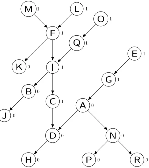
Although there are many types of feature selection methods for classifica-tion [47,84,96], in general these methods have the limitation that they do not exploit information associated with the hierarchy (generalisation-specialisation re-lationships) among features, which present in some types of features. As the example shown in Figure 1.1, those features like J, H, D, B, A, C, etc., are hier-archically structured as a Directed Acyclic Graph (DAG), where feature J is the parent of features H and D, and both of them are the parent of feature B, while feature A is the child of features D and C.

This type of hierarchical relationships are relatively common (although usu-ally ignored) in applications. In text mining, for instance, features usuusu-ally repre-sent the presence or absence of words in a document, and words are involved in generalisation-specialisation relationships [31,91]; in bioinformatics, which is the type of application this thesis focuses on, the functions of genes or proteins are of-ten described by using a hierarchy of terms, where terms representing more generic

(19)

J

K

H

D

C

B

A

G

F

E

I

L

0 1 1 1 1 0 1 0 1 0 0 0

Figure 1.1Example of a Small DAG of Features

functions are ancestors of terms representing more specific functions. As another example of hierarchical features, many datasets in financial or marketing applica-tions (where instances represent customers) have the address of the customer as a feature. This feature can be specified at several hierarchical levels, varying from the most detailed level (e.g. the full post code) to more generic levels (e.g. the first two or first three digits of the post code).

From another perspective, hierarchies of features can also be produced by using hierarchical clustering algorithms [129] to cluster features, rather than to cluster instances, based on a measure of similarity between features. The basic idea is that each object to be clustered would be a feature, and the similarity between any two features would be given by a measure of how similar the values of those fea-tures are across all instances. For instance, consider a dataset where each instance represents an email, and each binary feature represents the presence or absence of a word. Two features (words) can be considered similar to the extent that they occur (or don’t occur) in the same sets of emails. Then, a hierarchical clustering algorithm can be used to produce a hierarchy of features, where each leaf clus-ter will consist of a single word, and higher-level clusclus-ters will consist of a list of words connected by an “or” logical operator. For example, if words “money” and “buy” were merged into a cluster by the hierarchical clustering algorithm, when mapping the original features to the hierarchical features created by the cluster-ing algorithm, an email with word “money” but without the word “buy” would be considered to have value “yes” for feature “money”, value “no” for feature “buy”,

(20)

and value “yes” for feature “money or buy”. Note that in this example the “or” operator was used (as opposed to the “and” operator) in order to make sure the feature hierarchy is a “IS-A” hierarchy; i.e. if an email has value “yes” for a feature, it will necessarily have value “yes” for all ancestors of that feature in the hierarchy. Intuitively, in datasets where such hierarchical relations among features exist, ignoring such relationships seems a sub-optimal approach; i.e. these hierarchical relationships represent additional information about the features that could be exploited to improve the predictive performance associated with feature selection methods – i.e. the ability of these methods to select features that maximise the predictive accuracy to be obtained by classification algorithms using the selected features. This is the basic idea behind the hierarchical feature selection methods proposed in this thesis.

The proposed hierarchical feature selection methods perform “lazy learning”, in the sense that they postpone the feature selection process to the moment when testing instances are observed, rather than in the training phase of conventional learning methods (which perform “eager learning”). The proposed methods are evaluated together with lazy learning versions of Bayesian network classifiers (al-though other types of lazy learning classifiers could be used in feature research).

In terms of applications of the proposed hierarchical feature selection meth-ods, this thesis focuses on analysing biological data about ageing-related genes [27,30,35,54,82,122–124]. The causes and mechanisms of the biological process of ageing are a mystery that has puzzled humans for a long time. Biological research has, however, revealed some factors that seem associated with the ageing process. For instance, caloric restriction – which consists of taking a reduced amount of calories without undergoing malnutrition – extends the longevity of many species [88]. In addition, research has identified that several biological pathways seem to regulate the process of ageing (at least in model organisms), such as the well-known insulin/insulin-like growth factor (IGF-1) signalling pathway [68]. It is also known that mutations in some DNA repair genes lead to accelerated ageing syn-dromes [34]. Despite such findings, ageing is a highly complex biological process which is still poorly understood, and much more research is needed in this area.

Unfortunately, conducting ageing experiments in humans is very difficult, due to the complexity of the human genome, the long lifespan of humans, and eth-ical issues associated with experiments with human. Therefore, research on the

(21)

biology of ageing is usually done with model organisms like yeast, worms, flies or mice, which can be observed in an acceptable time and have considerably simpler genomes. In addition, with the growing amount of ageing-related data on model organisms available on the web, in particular related to the genetics of ageing, it is timely to apply data mining methods to that data [123], in order to try to discover patterns that may assist ageing research.

More precisely, in this work, the instances being classified are genes from four major model organisms, namely: C. elegans,S. cerevisiae,D. melanogaster andM. musculus. Each gene has to be classified into one of two classes: pro-longevity or anti-longevity, based on the values of features indicating whether or not the gene is associated with each of a number of Gene Ontology (GO) terms, where each term refers to a type of biological process, molecular function or cellular component. Pro-longevity genes are those whose decreased expression (due to knockout, muta-tions or RNA interference) reduces lifespan and/or whose overexpression extends lifespan; accordingly, anti-longevity genes are those whose decreased expression extends lifespan and/or whose overexpression decreases it [111].

We adopt GO terms as features to predict a gene’s effect on longevity because of the widespread use of the GO in gene and protein function prediction and the fact that GO terms were explicitly designed to be valid across different types of organisms [112]. GO terms are organised into a hierarchical structure where, for each GO term t, its ancestors in the hierarchy denote more general terms (i.e. more general biological processes, molecular function or cellular component) and its descendants denote more specialised terms than t. It is important to consider the hierarchical relationships among GO terms when performing feature selec-tion, because such relationships encode information about redundancy among GO terms. In particular, if a given gene g is associated with a given GO term t, this logically implies that is also associated with all ancestors of t in the GO hierarchy. This kind of redundancy can have a substantially negative effect on the predictive accuracy of Bayesian network classification algorithms, such as Naïve Bayes [129]. This issue will be discussed in detail later.

(22)

1.1 An Overview of Original Contributions

This thesis makes original contributions in terms of proposing and empirically eval-uating four hierarchical feature selection methods, including three filter methods (which run in a data pre-processing phase, independent of the classifier), described in Chapter 4; and one embedded method (i.e. a method that performs the fea-ture selection process as part of the process of building the classifier), described in Chapter 5. In addition to these hierarchical feature selection methods, two algo-rithms for constructing the network topology of a Bayesian Network Augmented Naïve Bayes classifier are also proposed and empirically evaluated in Chapter 6. Both these methods are based on the features selected by conventional flat or the new hierarchical feature selection methods. Note that these contributions, which are the main contributions of this thesis, are contributions to the area of machine learning/data mining.

As another type of contributions, which are contributions to the area of the biology of ageing, we have created new datasets of ageing-related genes with hier-archical features, in order to evaluate the proposed hierhier-archical feature selection methods. In addition, these methods were applied to the created datasets, and the results were used to produce rankings of biological features.

1.2 Structure of This Thesis

This thesis is structured into 7 chapters, including the currentIntroduction Chap-ter. A brief description of the remaining chapters is presented next.

• Chapter 2 - Background on Data Mining

This chapter presents a review of data mining concepts and methods relevant for this research, especially focusing on the classification task. Conventional types of Bayesian network classification algorithms, e.g. Naïve Bayes and some Semi-naïve Bayes classifiers will be discussed. Moreover, feature selec-tion methods for classificaselec-tion will also be discussed in detail.

• Chapter 3 - Background on Biology of Ageing and Bioinformatics

(23)

ageing and bioinformatics, especially focusing on the task of gene/protein function prediction. Then, related works about ageing-related gene/protein function prediction using machine learning/data mining methods as well as work on classification methods applied to the biology of ageing will be reviewed.

• Chapter 4 - Lazy Hierarchical Feature Selection Methods with

Naïve Bayes

This chapter presents a detailed description of three proposed filter hierar-chical feature selection methods, followed by the empirical evaluation of their predictive performance when working with the Naïve Bayes classifier, in a number of ageing-related datasets. This chapter also presents the methods used to create the ageing-related datasets that were used in our experiments. In addition, this chapter also reports a ranking of ageing-related GO terms, based on the results of one of the best performing hierarchical feature selec-tion methods.

• Chapter 5 - Lazy Hierarchical Feature Selection Methods with Tree

Augmented Naïve Bayes (TAN)

This chapter presents a detailed description of one proposed embedded hier-archical feature selection method based on the Tree Augmented Naïve Bayes (TAN) classifier, followed by the empirical evaluation of its predictive perfor-mance by comparing it with other feature selection methods (including the filter hierarchical feature selection methods proposed in Chapter 4), when working with the Tree Augmented Naïve Bayes (TAN) classifier. This chap-ter also reports a ranking of ageing-related GO chap-terms, based on one of the best performing hierarchical feature selection methods combined with the TAN classifier.

• Chapter 6 - Lazy Hierarchical Feature Selection Methods with

Bayesian Network Augmented Naïve Bayes (BAN)

This chapter presents a detailed description of two algorithms proposed for constructing the network topology of a Gene Ontology-based Bayesian Net-work Augmented Naïve Bayes (GO–BAN), based on the features selected by either flat or hierarchical feature selection methods. This chapter also

(24)

conducts an empirical evaluation of both proposed algorithms. In addi-tion, this chapter includes a comparison between the best performing hi-erarchical feature selection methods when working with different Bayesian network classifiers, i.e. Naïve Bayes, Tree Augmented Naïve Bayes and Gene Ontology-based Bayesian Network Augmented Naïve Bayes.

• Chapter 7 - Conclusions and Future Work

This chapter concludes the thesis by summarising its contributions to the area of machine learning/data mining (primary contribution) and the area of biology/bioinformatics of ageing research (secondary contribution). In addition, further research directions are suggested.

1.3 List of Publications

The publications derived from this thesis consist of one journal paper, two con-ference papers and one abstract. In addition, one journal paper is in preparation. The detailed information about these papers is listed below.

Peer-Reviewed Journal Paper:

• C. Wan, A. A. Freitas, and J. P. de Magalhães, “Predicting the Pro-longevity

or Anti-longevity Effect of Model Organism Genes With New Hierarchical Feature Selection Methods”, IEEE/ACM Transactions on Computa-tional Biology and Bioinformatics (TCBB), 12(2), pp. 262–275, Mar.– Apr., 2015. DOI: 10.1109/TCBB.2014.2355218.

Note: This paper is a major extension of the IEEE BIBM conference paper, whose details are mentioned later.

Journal Paper in Preparation:

• C. Wanand A. A. Freitas, “An Empirical Evaluation of Hierarchical Feature

Selection Methods in Datasets of Ageing-related Genes”.

(25)

• C. Wanand A. A. Freitas, “Prediction of the pro-longevity or anti-longevity

effect of Caenorhabditis Elegans genes based on Bayesian classification methods”, in Proceedings ofIEEE International Conference on Bioin-formatics and Biomedicine (BIBM 2013), Shanghai, China, Dec., 2013, pp. 373–380. (Acceptance rate: 19.6%, 60/306)

• C. Wanand A. A. Freitas, “Two Methods for Constructing a Gene

Ontology-based Feature Network for a Bayesian Network Classifier and Applications to Datasets of Aging-related Genes”, in Proceedings ofthe 6th _ACM

Confer-ence on Bioinformatics, Computational Biology, and Health In-formatics (ACM–BCB 2015), Atlanta, USA, Sept., 2015, pp. 27–36.

(Acceptance rate: 34.0%, 48/141)

Published Abstract:

• C. Wan and A. A. Freitas. Gene Ontology Hierarchy-based Feature

Se-lection. Features and Structures 2014 (FEAST 2014) Workshop

attached to the 22nd International Conference on Pattern Recog-nition (ICPR 2014), Stockholm, Sweden, Aug., 2014. (Abstract [125]; Poster and Oral Presentation)

(26)

Chapter 2 Background on Data Mining

2.1 Knowledge Discovery in Databases (KDD)

Due to the rapid growth of data from real world applications, it is timely to adopt Knowledge Discovery in Databases (KDD) methods to extract knowledge or valuable information from data. Indeed, KDD has already been successfully adopted in real world applications, both in science and in business.

KDD is a field of inter-disciplinary research across machine learning, statistics, databases, etc [37,50,129]. Broadly speaking, the KDD process can be divided into four phases. The first phase is selecting raw data from original databases according to a specific knowledge discovery task, e.g. classification, regression or clustering. Then the selected raw data will be input to the phase of data pre-processing (the second phase), which aims at processing the data into a form that could be efficiently used by the type of algorithm(s) to be applied in the data mining phase - such algorithms are dependent on the chosen type of knowledge discovery task. The data pre-processing phase includes data cleaning, data normalisation, feature selection and feature extraction, etc. The third phase is data mining, where a model will be built by running learning algorithms on the pre-processed data. In this work, we address the classification task, where the learning (classification) algorithm builds a classification model or classifier as will be explained later. The final phase is extracting the knowledge from the built classifier or model. Among those four phases of KDD, the focus of this research is on the data pre-processing

(27)

Chapter 2. Background on Data Mining 11

phase, in particular the feature selection task, where the goal is to remove the redundant or irrelevant features in order to improve the predictive performance of classifiers. The feature selection task will be reviewed later in this chapter.

2.2 Data Mining Tasks and Paradigms

Data Mining tasks are types of problems to be solved by a machine learning or data mining algorithm. The main types of data mining tasks can be categorized as classification, regression and clustering. The former two tasks (classification andregression) are also grouped as thesupervised learning paradigm, whereas the latter one (clustering) is categorised as unsupervised learning.

Supervised learning consists of learning a function from labeled training data [93]. The supervised learning process consists of two phases, i.e. the training phase and the testing phase. Accordingly, in the supervised learning process, the original dataset is divided into training and testing datasets. In the training phase, only the training dataset will be used for inferring the specific function by learning a specific model, which will be evaluated by using the testing dataset in the testing phase.

Unlike supervised learning, unsupervised learning is usually defined as a process of learning particular patterns from unlabelled data. In unsupervised learning, there is no distinction between training and testing datasets, and all available data are used to build the model. The usual application of unsupervised learning is to find groups (or clusters)/patterns of similar instances, constituting a clustering problem.

2.2.1 Classification

The classification task is possibly the mostly studied task in data mining. It con-sists of building a classification model or classifier to predict the class label (a nominal or categorical value) of an instance by using the values of the features (predictor attributes) of that instance [37,50]. Actually, the essence of the clas-sification process is exploiting correlations between features and the class labels of instances in order to find the border between class labels in the data space - a

(28)

space where the position of an instance is determined by the values of the features in that instance. The classification border is exemplified in Figure 2.1, in the con-text of a problem with just two class labels, where the found classification border (a black dashed line) distinguishes the instances labelled as square or circle.

Figure 2.1 Example of Data Classifiertion into Two Categories [89]

Many types of classification algorithms have been proposed, such as Bayesian network classifiers, Decision Trees, Support Vector Machines (SVM), Artificial Neural Networks (ANN), etc. From the perspective of interpretability of the clas-sifier, those classifiers can be categorised into two groups, i.e. “white box” and “black box” classifiers. The “white box” classifiers, e.g. Bayesian network clas-sifiers and Decision Trees, have better interpretability than the latter ones, e.g. Support Vector Machine (SVM) and Artificial Neural Networks (ANN) [38]. In this thesis, we focus on Bayesian network classifiers [41,126,127,141,142] (more precisely, Naïve Bayes and Semi-naïve Bayes classifiers), due to their good poten-tial for interpretability; in addition to their ability to cope with uncertainty in data – a common problem in bioinformatics [44].

(29)

2.2.2 Regression

Regression analysis is a traditional statistical task with the theme of discovering the association between predictive variables (features) and the target (response) variable. As it is usually used for prediction, regression analysis can also be con-sidered a type of supervised learning task from the perspective of machine learning and data mining.

Overall, a regression method is capable of predicting the numeric (real-valued) value of the target variable of an instance - unlike classification methods, which predict nominal (categorical) values, as mentioned earlier. A typical example of a conventional linear regression model for a dataset with just one featurex is shown as Equation 2.1,

yi =β0+β1xi+ξi (2.1)

where xi denotes the value of the feature x for the i-th instance, βi denotes the corresponding weight, and ξi denotes the error. The most appropriate values of the weights in Equation 2.1 can be found using mathematical methods, such as the well-known Linear Least Square [78,86,110]. Then the predicted output valueyi is computed based on the values of the input feature with its corresponding weight. As shown in the simple example of Figure 2.2, the small distances between the line and the data points indicates that Equation 2.1 fits well the data. Regression analysis has been well studied in the statistics area and widely applied in different domains.

(30)

Figure 2.2 Example of Regression for Data [56]

2.2.3 Clustering

The clustering task mainly aims at finding patterns in the data by grouping similar instances into clusters (or groups). The instances within the same cluster are more similar with each other, but simultaneously more dissimilar with the instances in other clusters. An example of clustering is shown in Figure 2.3, where the left graph represents the situation before clustering, where all data are unlabelled (in blue), and the right graph represents the situation where all data are clustered into three different groups, i.e. one group of data in blue, one group of data in red, and one group of data in green.

Clustering has been widely studied in the area of statistical data analysis, and applied on different domains, like information retrieval, bioinformatics, etc. Examples of well-known, classical clustering methods are k-means [51] and k-medoids [61].

(31)

Figure 2.3 Example of Data Clustered into Three Groups [99]

2.2.4 Eager and Lazy Learning Paradigms

Data mining or machine learning methods can be categorised into two general paradigms, depending on when the learning process is performed, namely: eager learning and lazy learning. An eager learning method performs the learning process during the training phase, i.e. learning the classifier (or classification model) using the whole training dataset before any testing instance is observed. Then the classifier is used to classify all testing instances. This is in contrast to the lazy learning approach, where the learning process is performed after observing the feature values for each individual testing instance in the testing phase. That is, a lazy learning-based classification algorithm builds a specific classification model for each individual testing instance to be classified [6,96].

In the context of feature selection, which is the research theme of this thesis and will be discussed in later sections, lazy learning-based methods select a specific set of features for each individual testing instance, whilst eager learning-based methods select a single set of features for all testing instances.

(32)

2.3 The Naïve Bayes (NB) Classifier

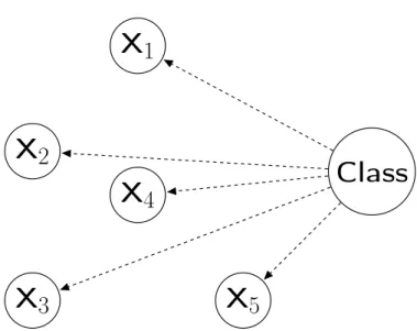
The Naïve Bayes classifier [37,50,92,95,129] is a type of Bayesian network classifier that assumes that all features are independent from each other given the class attribute. An example of this classifier’s network topology is shown in Figure 2.4, where each feature xi (i = 1,2, ...,5) only depends on the class attribute. In the figure, this is indicated by an edge pointing from the class node to each of the feature nodes. As shown in Equation 2.2,

P(y _|x₁, x₂, ..., xn)∝P(y) n Y i=1

P(xi |y) (2.2)

where _∝ is the mathematical symbol for proportionality and n is the number of features; the estimation of the probability of a class attribute value y given all predictor features’ values xi of one instance can be obtained by calculating the product of the individual probability of each feature value given a class attribute value and the prior probability of that class attribute value. Naïve Bayes (NB) has been shown to have relatively powerful predictive performance, compared with other Bayesian network classifiers [41], even thought it pays the price of losing the dependencies between features.

X

1 X

2 X

3 X

5 X

4 Class

(33)

2.4 Semi-naïve Bayes Classifiers

The Naïve Bayes classifier is very popular and has been applied on many domains due to its advantages of simplicity and short learning time, compared with other Bayesian classifiers. However, the assumption of conditional independence between features is usually violated in practice. Therefore, many extensions of Naïve Bayes focus on approaches to relax the assumption of conditional independence [41,73,

141]. This sort of classifier is called Semi-naïve Bayes classifier.

Both the Naïve Bayes classifier and Semi-naïve Bayes classifiers use estimation of the prior probability of the class and the conditional probability of the features given the class to obtain the posterior probability of the class given the features, as shown in the Equation 2.3 (i.e. the Bayes’ formula), where y denotes a class and x denotes the set of features, i.e. {x₁, x₂, ..., xn}. However, different Semi-naïve Bayes classifiers use different approaches to estimate the term P(x _| y), as discussed in the next subsections.

P(y_|x) = P(x|y)P(y)

P(x) (2.3)

2.4.1 Tree Augmented Naïve Bayes (TAN) and

SuperPar-ent Tree AugmSuperPar-ented Naïve Bayes (SP–TAN)

TAN constructs a network in the form of a tree, where each feature node is allowed to have at most one parent feature node in addition to the class node (which is a parent of all feature nodes), as shown in Figure 2.5, where each feature except the root feature X4 has only one non-class parent feature. TAN computes the posterior probability of a class y using Equation 2.4,

P(y _|x1, x2, ..., xn)∝P(y) n Y i=1

P(xi |P ar(xi), y) (2.4)

where the number of non-class parent features for each feature xi (i.e. P ar(xi)), except the root feature, equals to “1”. Hence, it represents a limited degree of dependencies among features.

(34)

X

1 X

2 X

3 X

5 X

4 Class

Figure 2.5An Example of TAN’s Network Topology

In essence, the original TAN classifier firstly produces a rank of feature pairs according to the conditional mutual information between the pair of features given the class attribute. Then the Maximum Spanning Tree is built based on the rank. Next, the algorithm randomly chooses a root feature and then sets all directions of edges to other features from it. Finally, the constructed tree is used for classi-fication.

The concept of conditional mutual information proposed for building TAN clas-sifiers is an extension of mutual information. The formula of conditional mutual information is shown as Equation 2.5,

Ip(Xi;Xj |Y) = X xi,xj,y P(xi, xj, y)log P(xi, xj |y) P(xi |y)P(xj |y) (2.5)

where Xi and Xj are predictor features, Y is the class attribute, xi, xj, y are the values of the corresponding features and the class attribute, P(xi, xj, y) denotes the joint probability of xi, xj, y; P(xi, xj | y) denotes the joint probability of fea-ture values xi and xj given class value y; and P(xi | y) denotes the conditional probability of feature value xi given class value y. Each pair of features “xi, xj” is taken into account as a group, then the mutual information for each pair of features given the class attribute is computed [41].

As a variant of TAN, SuperParent-TAN (SP–TAN) adopts the wrapper ap-proach to build the feature tree. More precisely, it tentatively makes each feature

(35)

node as theSuperParent in turn. TheSuperParent is a node that has arcs to every orphan node, i.e. every node that currently has no feature parent. Then, the node that mostly improves the predictive accuracy by leave-one-out cross validation will be selected as the SuperParent Asp. After selecting the unique SuperParent fea-ture, the selection of its favorite orphan is conducted. Thefavorite orphan is the feature which mostly improves the predictive accuracy, if it is connected with the SuperParent. Then an arc will be connected from Asp to its favorite orphan. The process above will be repeated until there is no improvement on accuracy or the number of remaining orphans equals to one [69].

In terms of the type of classification model finally built, the original TAN randomly selects a root node of the Maximum Spanning Tree, whereas SP–TAN selects aSuperParent node as the root by taking into account the predictive per-formance of the feature tree. In the topology of the network built by TAN, the number of arcs equals to n - 1 (n denotes the number of nodes), whereas the number of arcs made by SP–TAN might be fewer. According to the experimental results reported in [69], SP–TAN outperforms TAN in most cases for the datasets adopted in the experiments.

2.4.2 Bayesian Network Augmented Naïve Bayes (BAN)

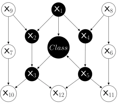
The BAN classifier is a more complicated type of Semi-naïve Bayes classifier, which (unlike NB and TAN) can represent more complicated dependencies between features [23,41]. More precisely, in a BAN, in Equation 2.4, the number of parent feature node(s) for each nodexi (i.e. P ar(xi)) is allowed to be more than one. An example of this classifier’s network topology is shown in Figure 2.6, where each feature xi has the class attribute as a parent, indicated by the dashed lines; and possibly other non-class parent feature(s), as indicated by the solid lines. NodeX₄

has two non-class parent nodesX1 and X5, while node X3 also has two non-class parent nodesX₂ and X₄.

There exist several approaches for constructing a BAN classifier from data that have been shown to be relatively efficient to use, particularly when the number of feature parents of a node is limited to a small integer number (a user-specified parameter). However, in general, learning a BAN classifier tends to be much more time consuming than learning a NB or TAN classifier, mainly due to the large

(36)

X

1 X

2 X

3 X

5 X

4 Class

Figure 2.6 An Example of BAN’s Network Topology

time taken to search for a good BAN network topology.

Fortunately, in the context of the bioinformatics data used in this project, there are strong dependency relationships between features, which have been already de-fined by expert biologists in the form of a feature graph, containing hierarchical relationships among features that are represented as directed edges in the feature graph (as will be explained in detail later). Such hierarchical relationships pro-vide a sophisticated representation of biological knowledge that can be directly exploited by a BAN classifier. Hence, we will use the pre-defined hierarchical rela-tionships retained in the data as the topology of the BAN classifier network, rather than learning the BAN network topology from the data, as will be discussed in Chapter 6.

2.4.3 Average One-Dependence Estimators (AODE)

Figure 2.7 An Example of AODE’s Network Topology

dependencies between the class attribute and all features.

In order to avoid the inaccurate estimation of probabilities caused by few in-stances, the minimal number of instances that have each value of the parent feature was set to 30, due to concerns on statistical significance. AODE computes the pos-terior probability of class valuey given the values of the set of featuresx as shown in Equation 2.6, P(y _|x)_∝ P i∈NVF(xi)≥mP(y, xi) Q j∈N,j6=iP(xj |y, xi) |i:_{i_∈NV F(x_i)_≥m_}| (2.6)

(38)

wherexi denotes each possible parent feature for all other features,xj denotes one of the features in the set of features except the parent feature xi, F(xi) denotes the number of instances associated with different values of the parent feature x_i,

N denotes the set of feature indices and m is a user-defined parameter – set to 30 in the original work proposing AODE, as mentioned earlier.

In terms of alleviating the problem of the feature independence assumption for Naïve Bayes, the AODE algorithm has the advantages of simplicity and theoret-ical foundation. But it has the disadvantage that the model’s interpretability is hindered by the fact that the final model actually consists of a large number of one-dependency models (one such model for each predictor feature used as parent for all other features).

2.4.4 Naïve Bayes Tree (NBTree)

The NBTree classifier [72] is a hybrid classifier combining Naïve Bayes and Decision Tree classifiers. It follows the idea of recursive partitioning of a dataset according to the values of features selected to discriminate among the classes, as performed by Decision Tree algorithms [37]. An important difference between NBTree and conventional Decision Tree algorithms is the evaluation function used for selecting features. NBTree uses the utility (rather than the entropy) of individual features as the criterion for selecting the splitting feature. The utility of a feature is measured by the predictive accuracy associated with individual tree nodes by using Naïve Bayes, where the predictive accuracy is estimated through 5-fold cross validation. In NBTree, for each leaf in the tree, the set of features can be divided into two feature subsets, namely the set of splitting features occurring in the path from the root to that leaf, and the remaining set of features (i.e. features not occurring in that path). The estimation of the posterior probability of the class value y given the set of values of the remaining features xi and the set of values of the splitting features x′ _{for a given leaf is given by Equation 2.7,}

P(y_|x, x′)_∝P(y, x′)Y i∈l

(39)

where x′ _{is the set of values of the set of splitting features in the path from the}

root to the current leaf, andl is the set of indices for the remaining features [141]. The utility of each split for an individual feature equals to the weighted sum of the utility of the new leaf nodes created by that split. For the sake of avoiding the over-fitting problem caused by splitting nodes with few instances, the process of recursively splitting the data terminates if the error reduction is below 5% or the number of instances in the current node to be split is less than 30.

According to the experimental results reported in [72], NBTree obtains high predictive accuracy in many cases, but its running time is not competitive against Naïve Bayes. In addition, the interpretability is a merit of NBTree, which is similar to an advantage of Decision Tree classifiers [38].

2.4.5 The Lazy Bayesian Rules (LBR) Algorithm

The Lazy Bayesian Rules (LBR) algorithm [143] follows the lazy learning approach, i.e. it builds a local Naïve Bayes classifier for each testing instance, rather than for the whole training dataset. A rule has the form: IF(antecedent),THEN(Class); where the Class in the rule’s consequent (THENpart) is predicted for instances satisfying the rule’s antecedent (IF part). The antecedent of a Bayesian rule is composed by a set of feature-value pairs with the form “f eature = value”. The utility of adding each feature-value pair into the antecedent is evaluated by leave-one-out cross validation and the best pair will be added into the antecedent if its associated classification error is lower than the error obtained by the existing local Naïve Bayes classifier created from the training dataset. This process terminates if there is no significant improvement on predictive performance. The inference formula used by LBR is shown as Equation 2.8,

P(y_|x, q)_∝P(y, q)Y i∈s

P(xi |y, q) (2.8)

where y denotes the class attribute value, q denotes the set of features’ values in the rule’s antecedent and s represents the set of indices of the remaining features. LBR’s criterion for stopping rule growing can naturally avoid the over-fitting problem by avoiding including in a rule antecedent an infrequent feature value, due

(40)

to its “lazy” learning approach. However, LBR uses cross validation to measure the predictive accuracy associated with each feature-value pair to be added to a rule, so it has a high processing time for growing the antecedent.

2.5 Conventional, “Flat” Feature Selection

Feature selection is a type of data pre-processing task that consists of removing irrelevant and redundant features in order to improve the predictive performance of classifiers. The role of feature selection methods in the classification process is illustrated by the flow-chart shown in Figure 2.8, where the dataset with the full set of features is input to the feature selection method, which will select a subset of features to be used for building the classifier. Then the built classifier will be evaluated, by measuring its predictive accuracy. Irrelevant features can be defined as features which are not correlated with the class variable, and so removing such features will not be harmful for the predictive performance. Redundant features can be defined as those features which are strongly correlated with other features, so that removing those redundant features should also not be harmful for the predictive performance.

Generally, feature selection methods can be categorised into three groups, i.e. wrapper approaches, filter approaches and embedded approaches, as discussed next.

Input

Dataset

Feature

Selection

Build

Classifier

Measure

Accuracy

Figure 2.8 Flow-Chart of the Classification Process Including Feature Selection in a Pre-Processing Phase

(41)

2.5.1 The Wrapper Approach

The wrapper feature selection approach decides which features should be selected from the original full set of features based on the predictive performance of the classifier with different candidate feature subsets. In the wrapper approach, the training dataset is divided into a “building” (or “learning”) set and a validation set. As summarised in graphical form in Figure 2.9, the best subset of features to be selected is decided by iteratively getting a candidate feature subset, building the classifier from the learning set, using only the candidate feature subset, and measuring accuracy in the validation set. The boolean function “End?” will check whether the selected subset of features satisfies the expected improvement on pre-dictive performance. If not so, the re-selection of a candidate feature subset will be conducted again, otherwise, the stage of feature selection will terminate, and the best subset of features will be used for building the classifier, which is finally evaluated on the testing dataset.

The wrapper approach selects features that tend to be tailored to the classifi-cation algorithm, since the feature selection process was guided by the algorithm’s accuracy. However, the wrapper approach has relatively higher time complex-ity than the filter and embedded approaches, since in the wrapper approach the classification algorithm has to be run many times.

One feature selection method following the wrapper approach is Backward Sequential Elimination (BSE). It starts with the full set of features, then iteratively uses leave-one-out cross validation to detect whether removing a certain feature, whose elimination will most reduce the training error on the validation set, will improve predictive accuracy. It repeats this process until the improvement in accuracy ends [141].

The opposite approach, named Forward Sequential Selection (FSS), starts with the empty set of features and then iteratively adds the feature that mostly im-proves accuracy on the validation dataset to the set of selected features. This iterative process is repeated until the predictive accuracy starts to decrease [76]. Both wrapper feature selection methods just discussed have a very high processing time because they perform many iterations and each iteration involves measuring predictive accuracy on the validation dataset by running a classification algorithm.

Novel Hierarchical Feature Selection Methods for Classification and Their Application to Datasets of Ageing-Related Genes

Kent Academic Repository

Full text document (pdf)

Citation for published version

Wan, Cen (2015) Novel Hierarchical Feature Selection Methods for Classification and Their

Application to Datasets of Ageing-Related Genes. Doctor of Philosophy (PhD) thesis, University

of Kent.

DOI

Link to record in KAR

http://kar.kent.ac.uk/54761/

Document Version

Novel Hierarchical Feature Selection

Methods for Classification and

Their Application to Datasets

of Ageing-Related Genes

Cen Wan

Contents

List of Figures

List of Tables

Abstract

Acknowledgements

Chapter 1

Introduction

J

K

H

D

C

B

A

G

F

E

I

L

1.1

An Overview of Original Contributions

1.2

Structure of This Thesis

1.3

List of Publications

Chapter 2

Background on Data Mining

2.1

Knowledge Discovery in Databases (KDD)

2.2

Data Mining Tasks and Paradigms

2.2.1

Classification

2.2.2

Regression

2.2.3

Clustering

2.2.4

Eager and Lazy Learning Paradigms

2.3

The Naïve Bayes (NB) Classifier

X

1

X

2

X

3

X

5

X

4

Class

2.4

Semi-naïve Bayes Classifiers

2.4.1

Tree Augmented Naïve Bayes (TAN) and

SuperPar-ent Tree AugmSuperPar-ented Naïve Bayes (SP–TAN)

X

1

X

2

X

3

X