AUTOMATIC ARRHYTHMIAS DETECTION USING VARIOUS TYPES OF ARTIFICIAL NEURAL NETWORK BASED LEARNING VECTOR
QUANTIZATION
Diane Fitria1, M. Anwar Ma’sum1, Elly Matul Imah2, and Alexander A.S. Gunawan 3 1Faculty of Computer Science, Universitas Indonesia, Kampus UI Depok, 16424, Indonesia 2Mathematics Department, State University of Surabaya, Jl. Ketintang, Surabaya, 60231, Indonesia
3Faculty of Computer Science, Bina Nusantara University, Jl. K H Syahdan No. 9 Jakarta, 11480, Indonesia
E-mail:[email protected] Abstract
An automatic Arrythmias detection system is urgently required due to small number of cardiologits in Indonesia. This paper discusses only about the study and implementation of the system. We use several kinds of signal processing methods to recognize arrythmias from ecg signal. The core of the system is classification. Our LVQ based artificial neural network classifiers based on LVQ, which includes LVQ1, LVQ2, LVQ2.1, FNLVQ, FNLVQ MSA, FNLVQ-PSO, GLVQ and FNGLVQ. Experiment result show that for non round robin dataset, the system could reach accuracy of 94.07%, 92.54%, 88.09% , 86.55% , 83.66%, 82.29 %, 82.25%, and 74.62% respectively for FNGLVQ, FNLVQ-PSO, GLVQ, LVQ2.1, FNLVQ-MSA, LVQ2, FNLVQ and LVQ1. Whereas for round robin dataset, system reached accuracy of 98.12%, 98.04%, 94.31%, 90.43%, 86.75%, 86.12 %, 84.50%, and 74.78% respectively for GLVQ, LVQ2.1, FNGLVQ, FNLVQ-PSO, LVQ2, FNLVQ-MSA, FNLVQ and LVQ1.
Keywords: Automatic Arrythmias detection, ECG, Classification, LVQ1, LVQ2, LVQ2.1, FNLVQ, FNLVQ MSA, FNLVQ-PSO, GLVQ, FNGLVQ
Abstrak
Sistem deteksi aritmia otomatis sangat diperlukan karena keterbatsan dokter spesialis jantung di Indinesia. Paper ini akan mendiskusikan secara lengkap tentang studi dan implementasi dari sistem tersebut. Kami menggunakan berbagai macam metode pengolahan sinyal untuk mengenali aritmia berdasarkan sinyal ekg. Bagian utama dari sistem adalah klasifikasi. Kami menggukanakn jaringan syaraf tiruan berbasis LVQ yang meliputi LVQ1, LVQ2, LVQ2.1, FNLVQ, FNLVQ MSA, FNLVQ-PSO, GLVQ dan FNGLVQ. Hasil eksperimen menunjukkan untuk data non round robin tingkat akurasi sistem mencapai 94.07%, 92.54%, 88.09% , 86.55% , 83.66%, 82.29 %, 82.25%, dan 74.62%d berturut-turut untuk FNGLVQ, FNLVQ-PSO, GLVQ, LVQ2.1, FNLVQ-MSA, LVQ2, FNLVQ dan LVQ1. Sedangkan untuk data round robin tingkat akurasi sistem mencapai 98.12%, 98.04%, 94.31%, 90.43%, 86.75%, 86.12 %, 84.50%, dan 74.78% berturut-turut untuk GLVQ, LVQ2.1, FNGLVQ, FNLVQ-PSO, LVQ2, FNLVQ-MSA, FNLVQ dan LVQ1.
Kata Kunci: Deteksi aritmia otomatis, EKG, klasifikasi, LVQ1, LVQ2, LVQ2.1, FNLVQ, FNLVQ MSA, FNLVQ-PSO, GLVQ, FNGLVQ
1. Introduction
Cardiac dysrhythmia or arrhythmia is an abnor-mality of the heart rhythm. In this disorder, the he-art rate may be too fast or just too slow com-parared to normal heart rate, which is about 60-80 beats per minute. In this disorder heart shythm also could be irregular [1]. Some types of arrhy-thmia are not dangerous even sometimes patients are unaware of the condition. In several cases, pa-tients may experience clinical symptoms such as
palpitations, dizziness, chest pain, unable to brea-the and even sudden death. However, a normal pe-rson may also experience symptoms similar but not including arrhythmia. For example, heart rate increases during exercise or palpitations when we feel scared or anxious. To detect this disease we need not only clinical diagnosis but also takes oth-er investigations. Common examination of heart is done by checking heart signal which utilize elec-trocardiogram (ECG) tools. The results of the exa-mination is the waves represent electrical activity
of the heart called ECG waves. These waves can describe the condition heart. But not everyone has the ability to translate the waves. In addition, the-re is a diffethe-rence of interpthe-retation between the ex-perts. Furthermore, the number of cardiologist in Indonesia is much smaller than the number of po-pulation, approximately 1:665.730 [2]. This facts motivated us to develop an early detection mecha-nism that easily can be used not only by expert but also by wider society. Mechanisms of the sys-tem is implemented using artificial intelligence to detect heart diseases based on ECG waveforms.
There have been many studies related to this topic. Yeap et. al. proposed backpropagation algo-rithm for arrhythmia detection based on ECG data [3]. Yeap used ECG data derived from the AHA database. Ozbay et al did similar work, but used data from the MIT-BIH as training data and the data from its own institutions as testing data [4]. Ghongade et al focused on comparison of various feature extraction methods for ECG data [5]. Ghongade compared Discrete Fourier Transform (DFT), Principle Component Analysis (PCA), Di-screte Wavelet Transform (DWT), and morpholo-gical features such as R-peak and QRS complex, then the result of features extraction was classified using Backpropagation algorithm.
The other previous studies was conducted by Made Agus et al., which develop new neural net-work algorithm named Fuzzy-Neuro Generalized Learning Vector Quantization (FNGLVQ) [6]. Th-ey modified previous algorithm named Genera-lized Learning Vector Quantization (GLVQ) with fuzzy membership function for vector references. GLVQ was proposed by Sato et al. in previous research [7]. The basic idea of GLVQ is applying gradient descent optimization to LVQ 2.1 in order to minimize misclassification error (MCE) du-ring training process. LVQ 2.1 is variant of Learn-ing Vector Quantization (LVQ) classifier [8]. LVQ is competitive based artificial neural network pro-posed by Kohonen [8]. The other variants of LVQ is LVQ 2 and LVQ 3 [8]. In other research, Be-nyamin et al applied fuzzy concept to LVQ algo-rithm resulting Fuzzy-Neuro Learning Vector Qu-antization (FNLVQ) [9]. They also made variant of FNLVQ by applying matrix similarity analysis (MSA) concept in training process. Later, Roch-matullah et al. proposed new improvement of FN-LVQ by applying Particle Swarm Optimization (PSO) method resulting FNLVQ-PSO [10].
The aim of this research is to develop an au-tomatic arrhythmias detection using ECG data (signal). ECG signal acquired from patient is pro-ccessed in several steps to extract features. Then, the signal is classified to several types of heart condition. In this research, we use several LVQ
based classifiers. This framework is used for early detection and monitoring system of heart disease. Therefore, system can detect arrhythmias symp-tom ausymp-tomatically from heart beat signal. The ap-plication of this framework is expected to help people to maintain their heart health.
The rest of the paper is organized as follows. Section 2 discusses structure of the framework for automatic arrhythmias detection and classifiers used in this research. Section 3 discusses about experiment results and analysis, and we draw con-clusion in Section 4.
2. Methods
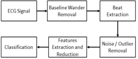
This section explain structure of proposed frame-work. Process sequence of proposed framework is shown in Figure 1. ECG signal will be processed in five steps. The first step is base-line wander re-moval which used to straighten ECG signal. The second process is beat extraction. Next, heart bea-ts from the same class was collected. Noises or outlier instances were removed from their class. Afterward, features were derived from each beat continued by features reduction. The last step is heart beat classification. Detail of each process will be explained in the following sub sections. Baseline Wandering Removal
The first phase of the ECG signal processing is Baseline Wander Removal (BWR). Baseline is a condition in which the ECG signal is not being isoelectric line (the axes) but shifted up or down. This phenomenon is caused by appearance of low frequency in heartbeat recording which come fr-om respiratory or body movements. Baseline of course will interfere analysis process of heartbeat signal and may lead to errors in the detection. Therefore it is necessary to remove the baseline.
A BWR process uses nonlinear cubic spline interpolation combined with reduction techniques (subtraction technique) so it can reduce noise wi-thout affecting ECG waveform significantly. The basic concept of BWR is shit estimation of main axis using representative points, one point for ea-ch beat, on the ECG waveform. Shit estimation of
major axis is done by cubic spline interpolation. Cubic interpolation is chosen because it can produce smoother signal. In addition, it can gua-rantee continuity of its first and second derivatives at the entire interval. Cubic spline interpolation is an estimation function that can be obtained using a third-degree polynomial in each sub-interval. Sub interval used in ECG signal is the PQ interval of each beat. After shift estimation of the main axis was obtained, then the real axis was deter-mined using isoelectric pivot. In this research we use BWR proposed by Clifford et al [11]. BWR process is shown on Figure 2.
Beat Extraction
In this research we use beat classification for arr-hythmias detection as used by previous researcher [12]. Using this approach, ECG signal is
segmen-ted in to collection of single beat. This approach is chosen because the dataset has annotation for R-peak. Segmentation result shows that the beat has 300 points. The result of beat segmentation is sho-wn in figure 3.
Noise/Outlier Removal
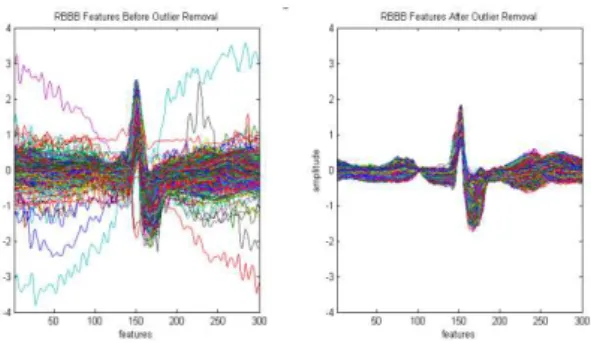
Beats segmented by previous steps are collected according their class label. Then, noises or outlier instances of each class were removed from data-set. In this research we used Inter Quarile Range method for noise/outlier removal which was used by previous researcher [6]. Sample of noise remo-val for class RBBB is shown in figure 4.
Feature Extraction and Reduction
A feature is information that used by classifier model to differentiate class of instances. There-fore, feature must be extracted from each instance of the dataset. In this research, we used Discrete Wavelet Transform (DWT) for features extraction. There are benefits can be obtained by using DWT. The first benefit is suitability of DWT for heart beat feature extraction. Arrhythmias can be detect-ed and recognizdetect-ed by recognizing pattern on the heartbeat. In other hand, DWT can be used to ac-quire information that represent signal pattern so it is suitable for heart beat feature extraction. The second benefit is DWT can reduce the dimension of the signal without losing important informa-tion. So it helped to obtain simpler computational process. The third benefit is DWT use filter opera-tion. Therefore signal produced by DWT is smoo-ther than original signal. In this research, we used Daubechies 8 (db8) mother wavelet for feature ex-traction.
The last process in the proposed framework is classification. Input of this process is feature extracted by previous process. The output of this process is prediction of the system for given sam-ple instances. We use LVQ based classifiers include LVQ1, LVQ2. LVQ2.1, GLVQ, FNLVQ,
Figure 2. Baseline Wander Removal Process
Figure 3. Beat segmentation result for class RBBB and class PVC
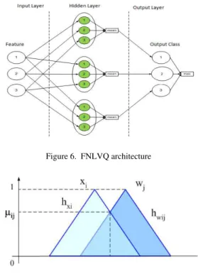
Figure 6. FNLVQ architecture
Figure 7. Computing similarity in FNLVQ
FNLVQ-MSA, FNLVQ-PSO, and FNG-LVQ. Classifiers
These sub-section explain the classifiers used in this research.
Learning Vector Quantization (LVQ)
Learning Vector Quantization (LVQ) is compete-tive based neural network proposed by Kohonen [8]. LVQ has two layers, input layer and output la-yer. LVQ Architecture is shown in Figure 5.
Let denote x as vector input, Y as class label, and 𝒘𝒘𝒊𝒊𝒊𝒊 as reference vector for class j element i (feature i). During training process, 𝒘𝒘𝒊𝒊𝒊𝒊is initiated by random value. Then iteratively, instance x was trained to the model. Next, distance of input vec-tor x and reverence vecvec-tor class j was computed using equation(1).
𝑑𝑑(𝑗𝑗) =�(𝑥𝑥𝑖𝑖−𝑤𝑤𝑖𝑖𝑖𝑖)2
𝑁𝑁 𝑖𝑖=1
(1)
After computing distance for all class, then we se-arch class with closest distance. Later, the class was called by winner class. Then reference vector of winner class 𝒘𝒘𝒑𝒑 was updated. Using equation (2).
𝑤𝑤𝑝𝑝← 𝑤𝑤𝑝𝑝+𝛼𝛼�𝑥𝑥 − 𝑤𝑤𝑝𝑝�𝑖𝑖𝑖𝑖𝐶𝐶𝑤𝑤𝑝𝑝=𝐶𝐶𝑖𝑖 (2) 𝑤𝑤𝑝𝑝← 𝑤𝑤𝑝𝑝− 𝛼𝛼�𝑥𝑥 − 𝑤𝑤𝑝𝑝�𝑖𝑖𝑖𝑖𝐶𝐶𝑤𝑤𝑝𝑝≠ 𝐶𝐶𝑖𝑖 (3)
Where 𝜶𝜶is learning rate, 𝑪𝑪𝒘𝒘𝒑𝒑is class label of wi-nner class and 𝑪𝑪𝒊𝒊is class label of sample x. LVQ 2
The basic concept of LVQ 2 is similar with LIVQ 1. LVQ 2 update winner reference vector (𝒘𝒘𝒑𝒑) and also runner up reference vector (𝒘𝒘𝒓𝒓) . LVQ 2 also
define new constant (𝝎𝝎) that used for limitation between d(p) and d(r). D(p) is distance between winner vector and input vector, whereas d(r) is distance between runner up vector and input vec-tor. Update process will be conducted according to the gıven equatıon(4).
𝑑𝑑𝑝𝑝
𝑑𝑑𝑟𝑟> (1− 𝜔𝜔) 𝑎𝑎𝑎𝑎𝑑𝑑
𝑑𝑑𝑟𝑟
𝑑𝑑𝑝𝑝< (1− 𝜔𝜔)
(4) If condition as mentioned in equation(4) was ac-cepted, then those two reference vectors would be updated using equation(5) and equation(6).
𝑤𝑤𝑝𝑝← 𝑤𝑤𝑝𝑝− 𝛼𝛼�𝑥𝑥 − 𝑤𝑤𝑝𝑝� (5)
𝑤𝑤𝑟𝑟← 𝑤𝑤𝑟𝑟+𝛼𝛼(𝑥𝑥 − 𝑤𝑤𝑟𝑟) (6)
LVQ 2.1
LVQ 2.1 is variant of is LVQ 2that uses assump-tion that the winner label class is same as input la-bel class 𝑪𝑪𝒙𝒙= 𝑪𝑪𝒘𝒘𝒑𝒑. LVQ 2.1 uses condition writ-en in equation(7). 𝐶𝐶𝑤𝑤𝑟𝑟≠ 𝐶𝐶𝑤𝑤𝑝𝑝𝑎𝑎𝑎𝑎𝑑𝑑𝑚𝑚𝑖𝑖𝑎𝑎( 𝑑𝑑𝑟𝑟 𝑑𝑑𝑝𝑝 ,𝑑𝑑𝑝𝑝 𝑑𝑑𝑟𝑟 ) > (1− 𝜔𝜔) (1 +𝜔𝜔) (7)
Fuzzy-Neuro Learning Vector Quantization (FN-LVQ)
FNLVQ was developed from LVQ by applying fuzzy concept to reference vector. In previous
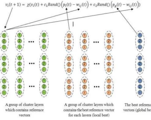
Figure 9. FNLVQ-PSO architecture
search, FNLVQ was proposed by Benyamin et al for artificial odor discrimination system [9]. FN-LVQ Architecture is shown in figure 6. There are three layers in FNLVQ, input layer, hidden layer and output layer. Input layer consists of input tor, hidden layer consists of class reference vec-tors, and output layer consists of output class of the input layer. Applying fuzzy concept, reference vector is represented by three values, i.e. 𝒘𝒘𝒊𝒊𝒊𝒊(𝒍𝒍),
𝒘𝒘𝒊𝒊𝒊𝒊,𝒘𝒘𝒊𝒊𝒊𝒊(𝒓𝒓) that represent min, mean, and max of the triangle.
Similar to other LVQ based neural network, FNLVQ use winner take all approach in training process. Reference vector will be updated based on winner vector, which is closest to the input. In FNLVQ, closest vector is obtained by computing similarity value from its fuzzy membership func-tion. Suppose that x is input vector, 𝒉𝒉𝒙𝒙 is fuzzy membership function of input vector x, 𝒘𝒘𝒊𝒊 is re-ference vector for class i, 𝒉𝒉𝒘𝒘𝒊𝒊 is fuzzy member-ship function of reference vector 𝒘𝒘𝒊𝒊, then simila-rity value between input vector and reference vec-tor can be computed using fuzzy triangle as sho-wn in Figure 7 [9].
Mathematically, similarity value for feature j in class i 𝝁𝝁𝒊𝒊𝒊𝒊can be computed using equation(8).
µij = max( hxj Λ hwij). (8) Then, similarity value for class i can be computed using equation(9).
µj = min(µij). (9)
Update process of reference vector is con-ducted according three conditions. First, if winner class is same as input label class, then reference vector will be updated using equation(10) to equa-tion(13).
𝑑𝑑𝑖𝑖𝑖𝑖← 𝛼𝛼 ∗(({1− 𝜇𝜇𝑖𝑖})∗(�𝑥𝑥𝑖𝑖− 𝑤𝑤𝑖𝑖𝑖𝑖(𝑡𝑡)�)) (10)
𝑤𝑤𝑖𝑖𝑖𝑖 ← 𝑤𝑤𝑖𝑖𝑖𝑖+𝑑𝑑𝑖𝑖𝑖𝑖 (11)
𝑤𝑤(𝑙𝑙)𝑖𝑖𝑖𝑖← 𝑤𝑤(𝑙𝑙)𝑖𝑖𝑖𝑖+𝑑𝑑𝑖𝑖𝑖𝑖 (12)
𝑤𝑤(𝑟𝑟)𝑖𝑖𝑖𝑖 ← 𝑤𝑤(𝑟𝑟)𝑖𝑖𝑖𝑖+𝑑𝑑𝑖𝑖𝑖𝑖 (13) Then, equation(12) to equation(13) are followed by widening or narrowing of the fuzzy triangle us-ing equation(14) and equation(15).
𝑤𝑤(𝑙𝑙)𝑖𝑖𝑖𝑖← 𝑤𝑤(𝑙𝑙)𝑖𝑖𝑖𝑖+ (𝛽𝛽 ∗(𝑤𝑤𝑖𝑖𝑖𝑖− 𝑤𝑤(𝑙𝑙)𝑖𝑖𝑖𝑖)) (14)
𝑤𝑤(𝑟𝑟)𝑖𝑖𝑖𝑖← 𝑤𝑤(𝑟𝑟)𝑖𝑖𝑖𝑖−(𝛽𝛽 ∗(𝑤𝑤(𝑟𝑟)𝑖𝑖𝑖𝑖− 𝑤𝑤𝑖𝑖𝑖𝑖)) (15) Second, if vector class is not same as input label class, then reference vector will be updated using equation(16) to equation(19).
𝑤𝑤𝑖𝑖𝑖𝑖 ← 𝑤𝑤𝑖𝑖𝑖𝑖− 𝑑𝑑𝑖𝑖𝑖𝑖 (17)
𝑤𝑤(𝑙𝑙)𝑖𝑖𝑖𝑖← 𝑤𝑤(𝑙𝑙)𝑖𝑖𝑖𝑖− 𝑑𝑑𝑖𝑖𝑖𝑖 (18)
𝑤𝑤(𝑟𝑟)𝑖𝑖𝑖𝑖 ← 𝑤𝑤(𝑟𝑟)𝑖𝑖𝑖𝑖− 𝑑𝑑𝑖𝑖𝑖𝑖 (19) Then, equations(18) and equation(19) are follow-ed by widening or narrowing of the fuzzy triangle using equation(20) and equation(21).
𝑤𝑤(𝑙𝑙)𝑖𝑖𝑖𝑖← 𝑤𝑤(𝑙𝑙)𝑖𝑖𝑖𝑖+ (𝛽𝛽 ∗(𝑤𝑤𝑖𝑖𝑖𝑖− 𝑤𝑤(𝑙𝑙)𝑖𝑖𝑖𝑖)) (20)
𝑤𝑤(𝑟𝑟)𝑖𝑖𝑖𝑖← 𝑤𝑤(𝑟𝑟)𝑖𝑖𝑖𝑖−(𝛽𝛽 ∗(𝑤𝑤(𝑟𝑟)𝑖𝑖𝑖𝑖− 𝑤𝑤𝑖𝑖𝑖𝑖)) (21) Third, if winner class is same as input label class, but similarity value is 0, then reference vec-tor will be updated using equation(12) to equation (15), followed by widening and narrowing fuzzy triangle using equation(22) and equation(23).
𝑤𝑤(𝑙𝑙)𝑖𝑖𝑖𝑖← 𝑤𝑤(𝑙𝑙)𝑖𝑖𝑖𝑖−(𝛽𝛽 ∗(𝑤𝑤𝑖𝑖𝑖𝑖− 𝑤𝑤(𝑙𝑙)𝑖𝑖𝑖𝑖)) (22)
𝑤𝑤(𝑟𝑟)𝑖𝑖𝑖𝑖← 𝑤𝑤(𝑟𝑟)𝑖𝑖𝑖𝑖+ (𝛽𝛽 ∗(𝑤𝑤(𝑟𝑟)𝑖𝑖𝑖𝑖+𝑤𝑤𝑖𝑖𝑖𝑖)) (23) where α is learning rate, β is constant between 0 and 1. Testing process in FNLVQ is conducted to determine winner (closest) reference vector to the input. This winner vector is the result of system prediction.
Fuzzy-Neuro Learning Vector Quantization–Ma-trix Similarity Analysis (FNLVQ-MSA)
During training process, FNLVQ will stop after reach the number of epoch given as parameter. Matrix similarity analysis (MSA) can be used to determine when it will stop the iteration. MSA describes reference vector at an iteration. It can give similarity value of the reference vector at the iteration. Therefore, we can set threshold of simi-larity value in which system should stop training process. FLVQ-MSA was proposed by Benyamin et al [8] for artificial odor discrimination system. Structure of MSA is shown in Figure 8.
𝑴𝑴 = �
𝒎𝒎𝟏𝟏𝟏𝟏 ⋯ 𝒎𝒎𝒏𝒏𝟏𝟏
⋮ ⋱ ⋮
𝒎𝒎𝟏𝟏𝒏𝒏 ⋯ 𝒎𝒎𝒏𝒏𝒏𝒏
�
Each element of M, 𝒎𝒎𝒊𝒊𝒊𝒊 can be computed using equation(24). 𝑚𝑚𝑚𝑚𝑖𝑖= 1 𝑁𝑁 �max (𝑚𝑚𝑖𝑖𝑎𝑎(𝜇𝜇𝑖𝑖𝑖𝑖)(𝑘𝑘)) 𝑁𝑁 𝑘𝑘=1 (24)
where M is n x n dimension MSA, n is the number of output class, 𝝁𝝁𝒊𝒊𝒊𝒊 is similarity value. Training
process of FNLVQ–MSA can be executed using steps: 1) Initiate reference vector; 2) Compute ma-trix similarity analysis; 3) Train the model; 4) Co-mpute current MSA. If current MSA is better than previous MSA, update reference vector; 5) If si-milarity values are less than threshold and the number of iteration is less than epoch then go to step 3. Testing process in FNLVQ-MSA is same as in FNLVQ.
Fuzzy-Neuro Learning Vector Quantization–Parti-cle Swarm Optimization (FNLVQ-PSO)
In previous research, Rochmatullah et al optimiz-ed Fuzzy-Neuro Learning Vector Quantization with Particle Swarm Optimization algorithm re-sulting FNLVQ-PSO [10]. Optimization is used during training process. PSO is optimization algo-rithm that uses colony of agents to find optimum value [13]. Architecture of FNLVQ-PSO is shown in Figure 9 [10].
PSO is optimization algorithm that uses co-lony of agents to find optimum value [13]. Each particle will search optimum point using equation (25) and equation(26). 𝑉𝑉𝑖𝑖(𝑡𝑡)←γ . ( 𝑉𝑉𝑖𝑖(𝑡𝑡 −1) +𝑐𝑐1.𝑟𝑟𝑎𝑎𝑎𝑎𝑑𝑑().�𝑃𝑃𝑖𝑖(𝑡𝑡 −1)− 𝑋𝑋𝑖𝑖(𝑡𝑡 −1)� +𝑐𝑐2.𝑟𝑟𝑎𝑎𝑎𝑎𝑑𝑑( ).�𝑃𝑃𝑃𝑃(𝑡𝑡 −1)− 𝑋𝑋𝑖𝑖(𝑡𝑡 −1)� (25) 𝑋𝑋𝑖𝑖(𝑡𝑡)← 𝑋𝑋𝑖𝑖(𝑡𝑡 −1)+𝑉𝑉𝑖𝑖(𝑡𝑡) (26) where Vi(t) is current particle velocity, Vi(t-1) is previous particle velocity, Xi(t) is current particle position, Xi(t-1) is previous particle position, c1 and c2 are constant, γ is construction factor which has value between 0 and 1,Pi(t-1) is previous local base of the agent, and Pg(t-1) is previous global base. Local best is optimum point for a particle. So each particle has their own local best. Global best is optimum point for all particle. In other wo-rds, global best is the most optimum of local best points. In FNLVQ-PSO, particle is represented as reference vector. Target of the optimization is to find the optimum reference vector during training. Training process In FNLVQ-PSO can be executed using following steps: 1) Initialize reference vec-tor as much as the number of particle. In FNLVQ-PSO, reference vector is generated in several nu-mber called particle. So there are several candi-dates of reference vector; 2) Train FNLVQ algo-rithm in each particle. For each particle, compute similarity value between input vector and referen-ce vector; 3) Compute MSA in each particle. The MSA will have n x n size matrix where n is the numbers of output class; 4) Compute MSA and fitness using equation(27); 5) Compute local best
and global best; 6) Update reference vector using equation(28) and equation(29); 7) Update fuzzy membership function of each particle using equa-tion(30) and equation(31) where d_ij is distance between particle and input vector.
𝑖𝑖𝑘𝑘= � 𝑚𝑚𝑖𝑖𝑖𝑖 𝑛𝑛 𝑖𝑖=1 − �� � 𝑚𝑚𝑖𝑖𝑖𝑖 𝑛𝑛 𝑖𝑖=1 𝑖𝑖𝑖𝑖𝑖𝑖 ≠ 𝑗𝑗 𝑛𝑛 𝑖𝑖=1 � (27) 𝑤𝑤𝑖𝑖𝑖𝑖(𝑡𝑡+ 1) =𝑤𝑤𝑖𝑖𝑖𝑖(𝑡𝑡) + 𝑣𝑣𝑖𝑖(𝑡𝑡+ 1) (28) 𝑣𝑣𝑖𝑖(𝑡𝑡+ 1) =γ � 𝑣𝑣𝑖𝑖(𝑡𝑡) + 𝑐𝑐1.𝑟𝑟𝑎𝑎𝑎𝑎𝑑𝑑. (𝑝𝑝𝑙𝑙(𝑡𝑡)− 𝑤𝑤𝑖𝑖𝑖𝑖(𝑡𝑡)) + 𝑐𝑐2.𝑟𝑟𝑎𝑎𝑎𝑎𝑑𝑑. (𝑝𝑝𝑔𝑔(𝑡𝑡)− 𝑤𝑤𝑖𝑖𝑖𝑖(𝑡𝑡)) � (29) 𝑤𝑤(𝑙𝑙)𝑖𝑖𝑖𝑖(𝑡𝑡+ 1) =𝑤𝑤(𝑙𝑙)𝑖𝑖𝑖𝑖(𝑡𝑡) + 𝑑𝑑𝑖𝑖𝑖𝑖 (30) 𝑤𝑤(𝑟𝑟)𝑖𝑖𝑖𝑖(𝑡𝑡+ 1) =𝑤𝑤(𝑟𝑟)𝑖𝑖𝑖𝑖(𝑡𝑡) + 𝑑𝑑𝑖𝑖𝑖𝑖 (31) 8) Repeat step 2 to step 7 until reference vector reach convergence. Convergence also can be defi-ned when the number of epoch is reached. Generalize Learning Vector Quantization (GLVQ) Generalize Learning Vector Quantization (GLVQ) was proposed by Sato and Yamada [7]. Sato and Yamada modified LVQ 2.1 with minimization of cost function and misclassification error. They us-ed gradient descent for minimization process. In GLVQ, 𝒘𝒘𝟏𝟏is definedasthe reference vector of in-put vector class 𝑪𝑪𝒙𝒙= 𝑪𝑪𝒘𝒘𝟏𝟏, and 𝒘𝒘𝟐𝟐 is the closest reference class from different class 𝑪𝑪𝒙𝒙≠ 𝑪𝑪𝒘𝒘𝟐𝟐. Miss classification error is defined as equation(32).
𝜑𝜑(𝑥𝑥) = 𝑑𝑑1−𝑑𝑑2
𝑑𝑑1+𝑑𝑑2
(32) Where 𝒅𝒅𝟏𝟏 is distance between 𝒘𝒘𝟏𝟏 and input vec-tor x, 𝒅𝒅𝟐𝟐 is distance between 𝒘𝒘𝟐𝟐 and input vector x. The value of 𝝋𝝋(𝒙𝒙) will be positive if input vec-tor x is correctly classified by system and negative if input vector x is classified in to wrong class. Target of the learning process is to minimize cost function as defined in equation(33).
𝑆𝑆= ∑ 𝑖𝑖𝑁𝑁𝑖𝑖=1 (𝜑𝜑(𝑥𝑥)) (33) where f() is rising monotonic function. To minimi-ze S, 𝒘𝒘𝟏𝟏 and 𝒘𝒘𝟐𝟐 will be updated using steepest descent method as equation(34).
𝑤𝑤𝑖𝑖← 𝑤𝑤𝑖𝑖− 𝛼𝛼𝛿𝛿𝑤𝑤𝛿𝛿𝛿𝛿𝑖𝑖,𝑖𝑖= 1,2 (34) If discriminant function used is Euclidean, then equation(27) can be written as equation(35) and equation(36). 𝛿𝛿𝑆𝑆 𝛿𝛿𝑤𝑤1= 𝛿𝛿𝑆𝑆 𝛿𝛿𝜑𝜑 𝛿𝛿𝜑𝜑 𝛿𝛿𝑑𝑑1 𝛿𝛿𝑑𝑑1 𝛿𝛿𝑤𝑤1 = − 𝛿𝛿𝑖𝑖 𝛿𝛿𝜑𝜑 4𝑑𝑑2 (𝑑𝑑1+𝑑𝑑2)2(𝑥𝑥 − 𝑤𝑤1) (35) 𝛿𝛿𝑆𝑆 𝛿𝛿𝑤𝑤2= 𝛿𝛿𝑆𝑆 𝛿𝛿𝜑𝜑 𝛿𝛿𝜑𝜑 𝛿𝛿𝑑𝑑2 𝛿𝛿𝑑𝑑2 𝛿𝛿𝑤𝑤1 = −𝛿𝛿𝑖𝑖 𝛿𝛿𝜑𝜑 4𝑑𝑑1 (𝑑𝑑1+𝑑𝑑2)2(𝑥𝑥 − 𝑤𝑤2) (36)
Therefore, the rules of learning process can be written as equation(37). 𝑤𝑤1← 𝑤𝑤1+𝛼𝛼𝛿𝛿𝜑𝜑𝛿𝛿𝑖𝑖 4𝑑𝑑2 (𝑑𝑑1+𝑑𝑑2)2(𝑥𝑥 − 𝑤𝑤1) (37) 𝑤𝑤2← 𝑤𝑤2+𝛼𝛼𝛿𝛿𝜑𝜑𝛿𝛿𝑖𝑖 4𝑑𝑑2 (𝑑𝑑1+𝑑𝑑2)2(𝑥𝑥 − 𝑤𝑤2) (38)
In GLVQ algorithm, the monotonic function used is sigmoid function as written in equation below.
𝑖𝑖(𝜑𝜑,𝑡𝑡) = 1 1 +𝑒𝑒−𝜑𝜑𝜑𝜑 (39) 𝛿𝛿𝑖𝑖 𝛿𝛿𝜑𝜑=𝑖𝑖(𝜑𝜑,𝑡𝑡)(1− 𝑖𝑖(𝜑𝜑,𝑡𝑡)) (40)
Fuzzy-Neuro Generalize Learning Vector Quanti-zation (FNGLVQ)
Fuzzy-Neuro Generalize Learning Vector Quanti-zation (FNGLVQ) was proposed by Made Agus et al. They combine fuzzy concept to GLVQ algori-thm [6]. FNGLVQ architecture is illustrated in Fi-gure 10 [6].
First, they complement distant value into d = 1-µ, then substitute to equation 26 resulting equa-tion(41).
𝜑𝜑(𝑥𝑥) = µ2− µ1 2− µ2− µ1
(41)
whereµ𝟏𝟏 is similarity value between input vector and reference vector from same class 𝑪𝑪𝒙𝒙=𝑪𝑪𝒘𝒘𝟏𝟏, and µ𝟐𝟐 is similarity value between input vector and closest reference vector from different class
𝑪𝑪𝒙𝒙≠ 𝑪𝑪𝒘𝒘𝟐𝟐.
Then adjustment of reference vector is made based on similarity value, as defined in equation (42). 𝛿𝛿𝛿𝛿 𝛿𝛿𝑤𝑤𝑖𝑖= 𝛿𝛿𝛿𝛿 𝛿𝛿𝜑𝜑. 𝛿𝛿𝜑𝜑 𝛿𝛿𝜇𝜇. 𝛿𝛿𝜇𝜇 𝛿𝛿𝑤𝑤𝑖𝑖 (42)
triangu-Figure 10. FNGLVQ architecture
lar function 𝑤𝑤𝑖𝑖𝑖𝑖�𝑤𝑤𝑚𝑚𝑖𝑖𝑛𝑛,𝑖𝑖𝑖𝑖,𝑤𝑤𝑚𝑚𝑚𝑚𝑚𝑚𝑛𝑛,𝑖𝑖𝑖𝑖,𝑤𝑤𝑚𝑚𝑚𝑚𝑚𝑚,𝑖𝑖𝑖𝑖�, mem-bership function can be defined as the following equation(43). 𝜇𝜇=ℎ(𝑥𝑥,𝑤𝑤𝑚𝑚𝑖𝑖𝑛𝑛,𝑤𝑤𝑚𝑚𝑚𝑚𝑚𝑚𝑛𝑛,𝑤𝑤𝑚𝑚𝑚𝑚𝑚𝑚) = ⎩ ⎪ ⎨ ⎪ ⎧ 𝑥𝑥 − 𝑤𝑤𝑚𝑚𝑖𝑖𝑛𝑛 0 ,𝑥𝑥 ≤ 𝑤𝑤𝑚𝑚𝑖𝑖𝑛𝑛 𝑤𝑤𝑚𝑚𝑚𝑚𝑚𝑚𝑛𝑛− 𝑤𝑤𝑚𝑚𝑖𝑖𝑛𝑛,𝑤𝑤𝑚𝑚𝑖𝑖𝑛𝑛≤ 𝑥𝑥 ≤ 𝑤𝑤𝑚𝑚𝑚𝑚𝑚𝑚𝑛𝑛 𝑤𝑤𝑚𝑚𝑚𝑚𝑚𝑚− 𝑥𝑥 𝑤𝑤𝑚𝑚𝑚𝑚𝑚𝑚− 𝑤𝑤𝑚𝑚𝑚𝑚𝑚𝑚𝑛𝑛,𝑤𝑤𝑚𝑚𝑚𝑚𝑚𝑚𝑛𝑛≤ 𝑥𝑥 ≤ 𝑤𝑤𝑚𝑚𝑚𝑚𝑚𝑚 0 ,𝑥𝑥 ≥ 𝑤𝑤𝑚𝑚𝑚𝑚𝑚𝑚 (43)
Derivation of the membership function to (wmean) lead is divided into three conditions and lead to learning formula as the following equation (44). If 𝑤𝑤𝑚𝑚𝑚𝑚𝑚𝑚𝑛𝑛<𝑥𝑥 ≤ 𝑤𝑤𝑚𝑚𝑚𝑚𝑚𝑚𝑛𝑛 𝑤𝑤1(𝑡𝑡+ 1)← 𝑤𝑤1(𝑡𝑡)− 𝛼𝛼𝑥𝑥𝜹𝜹𝝋𝝋𝜹𝜹𝜹𝜹x 2.(1−𝜇𝜇2) (2−µ1−µ2)2.𝑥𝑥 � 𝑚𝑚−𝑤𝑤𝑚𝑚𝑖𝑖𝑚𝑚 (𝑤𝑤𝑚𝑚𝑚𝑚𝑚𝑚𝑚𝑚−𝑤𝑤𝑚𝑚𝑖𝑖𝑚𝑚)2� (44) 𝑤𝑤2(𝑡𝑡+ 1) ← 𝑤𝑤2(𝑡𝑡)𝛼𝛼𝑥𝑥𝜹𝜹𝝋𝝋𝜹𝜹𝜹𝜹x 2. (1− 𝜇𝜇1) (2− µ1− µ2)2 x� 𝑥𝑥 − 𝑤𝑤𝑚𝑚𝑖𝑖𝑛𝑛 (𝑤𝑤𝑚𝑚𝑚𝑚𝑚𝑚𝑛𝑛− 𝑤𝑤𝑚𝑚𝑖𝑖𝑛𝑛)2� (45) If 𝑤𝑤𝑚𝑚𝑚𝑚𝑚𝑚𝑛𝑛<𝑥𝑥<𝑤𝑤𝑚𝑚𝑚𝑚𝑚𝑚 𝑤𝑤1(𝑡𝑡+ 1) ← 𝑤𝑤1+𝛼𝛼𝑥𝑥𝜹𝜹𝝋𝝋 𝒙𝒙𝜹𝜹𝜹𝜹 2. (1− 𝜇𝜇2) (2− µ1− µ2)2 𝑥𝑥 �(𝑤𝑤 𝑤𝑤𝑚𝑚𝑚𝑚𝑚𝑚− 𝑥𝑥 𝑚𝑚𝑚𝑚𝑚𝑚− 𝑤𝑤𝑚𝑚𝑚𝑚𝑚𝑚𝑛𝑛)2� (46) 𝑤𝑤2(𝑡𝑡+ 1)←𝑤𝑤2(𝑡𝑡) − 𝛼𝛼𝑥𝑥𝛿𝛿𝜑𝜑𝛿𝛿𝑖𝑖x 2. (1− 𝜇𝜇1) (2− µ1− µ2)2 x� 𝑤𝑤𝑚𝑚𝑚𝑚𝑚𝑚− 𝑥𝑥 (𝑤𝑤𝑚𝑚𝑚𝑚𝑚𝑚− 𝑤𝑤𝑚𝑚𝑚𝑚𝑚𝑚𝑛𝑛)2� (47) If 𝑥𝑥 ≤ 𝑤𝑤𝑚𝑚𝑖𝑖𝑛𝑛 dan 𝑥𝑥 ≥ 𝑤𝑤𝑚𝑚𝑚𝑚𝑚𝑚 𝑤𝑤𝑖𝑖(𝑡𝑡+ 1)← 𝑤𝑤𝑖𝑖(𝑡𝑡) ,𝑖𝑖= 1,2 (48) where w1 is reference vector from same class as input vector 𝐶𝐶𝑚𝑚 =𝐶𝐶𝑤𝑤1, and w2 reference vector from different class 𝐶𝐶𝑚𝑚≠ 𝐶𝐶𝑤𝑤2. Update rules for wmin and wmax follow equation(49) and equation (50). 𝑤𝑤𝑚𝑚𝑖𝑖𝑛𝑛 ← 𝑤𝑤𝑚𝑚𝑚𝑚𝑚𝑚𝑛𝑛(𝑡𝑡+ 1) − �𝑤𝑤𝑚𝑚𝑚𝑚𝑚𝑚𝑛𝑛(𝑡𝑡)− 𝑤𝑤𝑚𝑚𝑖𝑖𝑛𝑛(𝑡𝑡)� (49) 𝑤𝑤𝑚𝑚𝑚𝑚𝑚𝑚← 𝑤𝑤𝑚𝑚𝑚𝑚𝑚𝑚𝑛𝑛(𝑡𝑡+ 1) − �𝑤𝑤𝑚𝑚𝑚𝑚𝑚𝑚𝑛𝑛(𝑡𝑡)− 𝑤𝑤𝑚𝑚𝑖𝑖𝑛𝑛(𝑡𝑡)� (50)
The value of α is between 0 and 1, and its value will decrease along with the value of num-ber iteration (t), as defined in equation(51).
𝛼𝛼(𝑡𝑡+ 1) =𝛼𝛼0× �1− 𝑡𝑡 𝑡𝑡𝑚𝑚𝑚𝑚𝑚𝑚�
(51)
To gain better performance, we use addition-nal rule to adjust wmin and wmax as defined in conditions below:
If μ1 > 0 or μ2 > 0, then at least one of two refe-rence vectors recognize the input, therefore if ϕ < 0 then increase fuzzy triangular width using equa-tio(52) and equation(53).
𝑤𝑤𝑚𝑚𝑖𝑖𝑛𝑛← 𝑤𝑤𝑚𝑚𝑚𝑚𝑚𝑚𝑛𝑛−(𝑤𝑤𝑚𝑚𝑚𝑚𝑚𝑚𝑛𝑛− 𝑤𝑤𝑚𝑚𝑖𝑖𝑛𝑛) 𝑥𝑥�1 + (𝛽𝛽.𝛼𝛼)� (52) 𝑤𝑤𝑚𝑚𝑚𝑚𝑚𝑚← 𝑤𝑤𝑚𝑚𝑚𝑚𝑚𝑚𝑛𝑛+ (𝑤𝑤𝑚𝑚𝑚𝑚𝑚𝑚− 𝑤𝑤𝑚𝑚𝑚𝑚𝑚𝑚𝑛𝑛) 𝑥𝑥�1 + (𝛽𝛽.𝛼𝛼)� (53)
If input class is recognized into wrong class (ϕ≥ 0), then decrease triangular width using equation (54) and equation(55). 𝑤𝑤𝑚𝑚𝑖𝑖𝑛𝑛← 𝑤𝑤𝑚𝑚𝑚𝑚𝑚𝑚𝑛𝑛−(𝑤𝑤𝑚𝑚𝑚𝑚𝑚𝑚𝑛𝑛− 𝑤𝑤𝑚𝑚𝑖𝑖𝑛𝑛) 𝑥𝑥�1−(𝛽𝛽.𝛼𝛼)� (54) 𝑤𝑤𝑚𝑚𝑚𝑚𝑚𝑚← 𝑤𝑤𝑚𝑚𝑚𝑚𝑚𝑚𝑛𝑛+ (𝑤𝑤𝑚𝑚𝑚𝑚𝑚𝑚− 𝑤𝑤𝑚𝑚𝑚𝑚𝑚𝑚𝑛𝑛) 𝑥𝑥�1−(𝛽𝛽.𝛼𝛼)� (55)
If μ1 = 0 and μ2 = 0, then it means both reference vector cannot recognize input vector. Therefore, fuzzy triangular vectors must be increased using equation(56) and equation(57) where γ is a cons-tant value of 0.1.
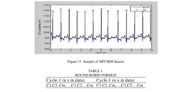
Figure 11. Sample of MIT-BIH dataset
TABLE 1. ROUND ROBIN FORMAT
Cycle-1 (n x m data) Cycle-1 (n x m data)
C1,C2..Cm,…,C1,C2…,Cm C1,C2..Cm,…,C1,C2…,Cm 𝑤𝑤𝑚𝑚𝑖𝑖𝑛𝑛← 𝑤𝑤𝑚𝑚𝑚𝑚𝑚𝑚𝑛𝑛−(𝑤𝑤𝑚𝑚𝑚𝑚𝑚𝑚𝑛𝑛− 𝑤𝑤𝑚𝑚𝑖𝑖𝑛𝑛) 𝑥𝑥�1−(γ.𝛼𝛼)� (56) 𝑤𝑤𝑚𝑚𝑚𝑚𝑚𝑚← 𝑤𝑤𝑚𝑚𝑚𝑚𝑚𝑚𝑛𝑛+ (𝑤𝑤𝑚𝑚𝑚𝑚𝑚𝑚− 𝑤𝑤𝑚𝑚𝑚𝑚𝑚𝑚𝑛𝑛) 𝑥𝑥�1 + (γ.𝛼𝛼)� (57)
3. Results and Analysis
In this research we used MIT-BIH Arrythmia da-tabase [14]. The dataset has 48 records from re-search subjects in BIH Arrithmia Laboratory. The dataset have been taken from 1975 to 1979. Each record has ± 3 minutes duration. Sample of the dataset is visualized in figure 11. The dataset used in this research consists of six class as, they are: 1) Normal beat (NOR); 2) Left Bundle Branch Block (LBBB); 3) Right Bundle Branch Block (RBBB); 4) Premature Ventricular Contraction (PVC); 5) Paced beat (PACE); 6) Atrial Prema-ture beat (AP).
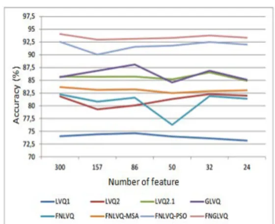
In this research, we use two experimental scenarios. The first scenario is conducted to mea-sure classifier performance according the number of features. The second scenario is used to measu-re impact of round robin data to performance cla-ssifier. In this experiment, learning rate was set to 0.05, and maximum epoch was set to 250. The re-sult of first scenario is shown in Figure 12.
We use six number of feature variation. Fi-gure 12 shows that FLGLVQ has the best perfor-mance among them for any number of features. The best accuracy reached by FNGLVQ is 94. 07%, when 300 features are used. FNLFQ-PSO is consistent in the second rank.
FNLVQ-PSO has best accuracy in 300 fea-tures dataset with 92.54 % accuracy. GLVQ and LVQ 2.1 compete in the third and fourth ranks. GLVQ reaches its best performance in 86 features dataset with 84.58 % accuracy, whereas LVQ2.1
has its best performance in 32 features dataset wi-th 86.55% accuracy. FNLVQ-MSA is consistent in fifth rank. It best accuracy is 83.66% which is in 300 features case. FNLVQ and LVQ2 compete for sixth and seventh rank. FNLVQ has best performance in 300 features dataset with 82.25% accuracy. LVQ2 reach its best performance in 32 features dataset with 82.29% accuracy. The worst classifier in this scenario is LVQ1. Its highest ac-curacy is 74.62% which is in 86 features data.
For the second scenario, we used 300 featu-res dataset, and six variation of round robin value. In round robin scenario, training data is formatted as table below. Cm is data with label class m, and n is number of round robin value.
The result of the second scenario is shown in Figure 13. Figure 13 shows that GLVQ surprising-ly has the best performance for any kind of round robin value. It reach best performance in 30 round robin data with 98.12% accuracy. FNGLVQ, LVQ 2.1, and FNLVQ-PSO compete for second, third and fourth ranks. FNGLVQ reached its best per-formance in 30 round robin case with 94.31% ac-curacy. LVQ2.1 also reached its best performance in 30 round robin case with 98.04% accuracy. Whereas FNLVQ-PSO reached its best perform-ance in 50 round robin case with 90.43% accu-racy. FNLVQ, FNLVQ-MSA, and LVQ2 compete for fifth, sixth, and seventh position. LVQ2 best accuracy is 86.75% which is in 50 round robin case. FNLVQ-MSA has best accuracy in 30 round robin case with 86.12, and so does the eighth posi-tion of FNLVQ 84.50% accuracy. The worst clas-sifier for round robin data is LVQ1 with 74.78% best accuracy in 50 round robin case. Overall, Fi-gure 3 shows that classifiers accuracy have been enhanced when round robin value was less than or equal to 50.
Figure 12. Classsifier performance according the number of feature (scenario-1)
Figure 13. Classsifier performance according the number ofround robin value (scenario-2)
From those scenarios we can say that round robin dataset has no significant improvement for classifiers with fuzzy membership function such as FNGLVQ, FNLVQ-PSO, FNLVQ-MSA, and FNLVQ. While it gives significant improvement for non-classifiers based on LVQ. When dataset is formatted as round robin, the sequence is always sorted as C1, C2, …, Cm. After update reference vector for input instance with C1 label, the next instance is always not C1. It causes classifiers gu-ess it as C1 which is wrong class. Therefore cla-ssifiers will widen its fuzzy triangle regarding the misclassification. Too wide fuzzy triangle is not good. It can cause misclassification. Therefore ro-und robin dataset give no significant improvement for classifiers with fuzzy
4. Conclusion
From the research performed, it can be concluded that automatic arrhythmias detection system has been successfully implemented. In this research, Arrhythmia dataset from MIT-BIH is used to mea-sure system performance. Result of first experi-ment said that for non-round robin dataset, the system can reach 94.07% accuracy with FNG-LVQ algorithm. It is followed by FNFNG-LVQ-PSO with 92.54% of accuracy, GLVQ with 88.09%, LVQ2.1 with 86.55%, FNLVQ-MSA with 83. 66%, LVQ2 with 82.29%, FNLVQ with 82.25%, and LVQ1 with 74.62% of accuracy. The result of the first experiment said that round robin data wi-th less wi-than or equal 50 can enhance accuracy. For round robin dataset, the system can reach 98.12% of accuracy with GLVQ algorithm. It is followed by LVQ2.1 with 98.04%, FNGLVQ with 94.31%, FNLVQ-PSO with 90.43%, LVQ2 with 86.75%, FNLVQ-MSA with 86.12 %, FNLVQ with 84. 50%, and LVQ1 with 74.78%.
References
[1] Bryg, R. M. "Heart Disease and Abnormal Heart Rhythm". 2009. http://www.webmd. com/heart-disease/guide/heart-disease-abnor mal-heart-rhythm?page=3
[2] Dicrease mortality caused by coronary heart disease. http://www.ugm.ac.id/en/berita/1593 -pengukuhan.prof.bambang.irawan%3A.upa ya.menurunkan.angka.kematian.akibat.jantu ng.koroneron March 2, 2014
[3] T. Yeap, F. Johnson, and M. Rachniowski, “ECG beat classification by a neural net-work,” in Engineering in Medicine and Bio-logy Society, 1990., Proceedings of the Twe-lfth Annual International Conference of the IEEE, pp. 1457 –1458, nov 1990.
[4] Y. Ozbay and B. Karlik, “A Recognition of ECG Arrhytihemias using artificial neural networks,” in Engineering in Medicine and Biology Society, 2001. Proceedings of the 23rd Annual International Conference of the IEEE, vol. 2, pp. 1680 – 1683 vol.2, 2001. [5] R. Ghongade and A. Ghatol, “A brief
per-formance evaluation of ECG feature extrac-tion techniques for artificial neural network based classification,” in TENCON 2007 - 2007 IEEE Region 10 Conference, pp. 1 –4, 30 2007-nov. 2 2007.
[6] Setiawan, I.M.A.; Imah, E.M.; Jatmiko, W., "Arrhytmia classification using Fuzzy-Neuro Generalized Learning Vector Quantization," Advanced Computer Science and Information System (ICACSIS), 2011 International Confe-rence on , vol., no., pp.385,390, 17-18 Dec. 2011.
[7] A. Sato and K. Yamada, “A formulation of learning vector quantization using a new misclassification measure,” in Proceedings of the 14th International Conference on Pattern
Recognition-Volume 1 - Volume 1, ICPR ’98, (Washington, DC, USA), pp. 322–, IEEE Computer Society, 1998
[8] T. Kohonen, “Learning Vector Quantization for Pattern Recognition,” Report TKK-F-A 601, Helsinki University of Technology, Es-poo, Finland, 1986.
[9] B. Kusumoputro, H. Budiarto, andW. Jatmi-ko, “Fuzzy-neuro LVQ and its comparison with fuzzy algorithm LVQ in artificial odor discrimination system,” ISA Transactions, vol. 41, no. 4, pp. 395 – 407, 2002.
[10] Jatmiko, W.; Rochmatullah; Kusumoputro, B.; Sanabila, H. R.; Sekiyama, K.; Fukuda, T., "Visualization and statistical analysis of fuzzy-neuro learning vector quantization based on particle swarm optimization for recognizing mixture odors," Micro-NanoMechatronics and Human Science,
2009. MHS 2009. International Symposium on , vol., no., pp.420,425, 9-11 Nov. 2009. [11] G. D. Clifford, “Baseline wander removal
open source ecg package,” 2005
[12] Ghongade and A. Ghatol, “A brief performance evaluation of ecg feature extraction techniques for artificial neural network based classification,” in TENCON 2007 - 2007 IEEE Region 10 Conference, pp. 1 –4, 30 2007-nov. 2 2007.
[13] Kennedy, J.; Eberhart, R. "Particle Swarm Optimization". Proceedings of IEEE International Conference on Neural Networks IV. pp. 1942–1948. (1995)
[14] G. B. Moody, “Mit-bih arrhythmia database.”
http://physionet.org/physiobank/database/ht ml/mitdbdir/mitdbdir.htm. May 1997.