http://www.scirp.org/journal/apm ISSN Online: 2160-0384 ISSN Print: 2160-0368
Nonlinear Evolution Equations and Its Application
to a Tumour Invasion Model
Akisato Kubo1, Yuto Miyata2, Hidetoshi Kobayashi3, Hiroki Hoshino1, Naoki Hayashi4
1Department of Mathematics, School of Health Sciences, Fujita Health University, Toyoake, Japan 2Medical Radiation Sciences, Graduate School of Health Sciences, Fujita Health University, Toyoake, Japan 3Department of Radiation Oncology, School of Medicine, Fujita Health University, Toyoake, Japan 4Faculty of Radiological Technology, School of Health Sciences, Fujita Health University, Toyoake, Japan
Abstract
We consider nonlinear evolution equations with logistic term satisfying initial Neu-mann-boundary condition and show global existence in time of solutions to the problem in arbitrary space dimension by using the method of energy. Applying the result to a mathematical model of tumour invasion, we discuss the property of the rigorous solution to the model. Finally we will show the time depending relationship and interaction between tumour cells, the surrounding tissue and matrix degradation enzymes in the model by computer simulations. It is seen that our mathematical re-sult of the existence and asymptotic behaviour of solutions verifies our simulations, which also confirm the mathematical result visibly.
Keywords
Nonlinear Evolution Equation, Mathematical Analysis, Tumour Invasion, Proliferation, Re-Establishment
1. Introduction
In this paper we consider the initial Neumann-boundary value problem of nonlinear evolution equations with logistic term, arising from tumour invasion models with pro-liferation and re-establishment: (NE)
(
)
(
)
(
)
( )
( )
( )
0( ) ( )
1( )
2
, e e 1 in 0, (1)
0 on 0, (2)
, 0 , , 0 in (3)
u u
t t t t
t
t
u D u u u u u T
u T
u x u x u x u x
χ µ
ν
− −
∂Ω
= ∆ + ∇ ⋅ ∇ + − Ω×
∂
= ∂Ω×
∂ = = ∂ Ω
How to cite this paper: Kubo, A., Miyata, Y., Kobayashi, H., Hoshino, H. and Haya-shi, N. (2016) Nonlinear Evolution Equa-tions and Its Application to a Tumour Inva-sion Model. Advances in Pure Mathematics, 6, 878-893.
http://dx.doi.org/10.4236/apm.2016.612066
Received: September 12, 2016 Accepted: November 14, 2016 Published: November 17, 2016
Copyright © 2016 by authors and Scientific Research Publishing Inc. This work is licensed under the Creative Commons Attribution International License (CC BY 4.0).
(
1)
1
2 2 2
, , 1, , , , ,
i n
n
t x x x
i
x x
i n u u u
t x
u u u u u
∂ = ∂ ∂ = ∂ = ⋅⋅⋅ ∇ = ∂ ∂
∂ ∂
∇ = ∇ ⋅ ∇ = ∆ = ∂ + ⋅⋅⋅ + ∂
where u:=u x t
( )
, for( )
x t, ∈ Ω ×( )
0,T , D and μ are positive constants, Ω is abounded domain in n
R and ∂Ω is a smooth boundary of Ω and ν is the outer unit
normal vector.
Let us introduce function spaces used in below. First, l
( )
H Ω denotes the usual
Sobolev space l,2
( )
W Ω of order l on Ω. For functions h x t
( )
, and k x t( )
, defined in Ω ×[
0,∞)
, we denote( )( )
( ) ( )
2( ) ( )( )
2( )
( ) ( )
2| |
, , , d , , , x ,
l
l
h k t h x t k x t x h t h h t h t βh t t
β ≤ Ω
=
∫
= =∑
∂ ⋅where β is a multi-index for β =
(
β1,⋅⋅⋅,βn)
.The eigenvalues of −∆ with the homogeneous Neumann boundary conditions are
denoted by
{
λi|i=0,1, 2,}
satisfying 0=λ0<λ1≤→ +∞ and ϕ ϕi = i( )
x in-dicates the 2L normalized eigenfunction corresponding to λi. For a non-negative
in-teger l, we set l
( )
W Ω as a closure of
{
ϕ ϕ1, 2,,ϕn,}
in the function space( )
lH Ω .
It is noticed that we have
∫
Ωh x( )
dx=0 for h x( )
∈Wl( )
Ω , which enables us to usePoincare’s Inequality.
Putting u x t
( )
, = + +a bt v x t( )
, in (1) it follows from (1) that(
)
(
)
( )(
)
(
)
2
, e a bt v ea bt v 1 2 1
t t t
tv D v χ b v v µv t b vt µb b
− − − − − −
= + ∇ ⋅ + + − +
∂ ∆ ∇ − −
where a and b are positive parameters. (NE) is rewritten by the following problem.
( )
[ ]
(
( )
)
(
)
(
)
( )
( )
( )
( )
2 ,
0 1
e 1 2 1 0,
RP 0,
, 0 , , 0 .
a b a bt v t
t
t t t
Q v v D v v v v b v b b
v
v x v x v x v x
χ µ µ
ν − − − ∂Ω = − ∆ − ∇ ⋅ ∇ − − − − = ∂ = ∂ = = ∂
-where a b,
( )
(
, e a bt v)
.t
v b v
χ =χ + − − −
We will show the global existence in time of solu-tions of (RP), which gives our desired result of (NE).
Applying the above result to the following mathematical model of tumour invasion proposed by Chaplain and Lolas [1], we have a rigorous mathematical understanding to tumour invasion for the key variables n, m and f .
(
)
(
)
(
)
(
)
(
)
1 2 1 (4)C-L 1 (5)
(6)
n n
m
n
d n x n m n f n n f
t f
mf f n f
t m
d m n m
t γ µ η µ α β ∂ = ∆ − ∇ ⋅ ∇ − ∇ ⋅ ∇ + − − ∂ ∂ = − + − − ∂ ∂ = ∆ + − ∂
In the right hand side of (4) the second, third and fourth terms mean chemotaxis, hap-totaxis and proliferation of tumour cell respectively. Also the second term of the right hand side of (5) describes the re-establishment of ECM. We consider an initial boun-dary value problem for (C-L) satisfying
(
)
0, on 0, ,
n f m
ν ν ν
∂ = ∂ =∂ = ∂Ω × ∞
∂ ∂ ∂
( )
, 0 0( ) ( )
, , 0 0( ) ( )
, , 0 0( )
n x =n x f x = f x m x =m x ,where
{
n0( ) ( )
x ,f0 x m, 0( )
x}
are initial data of{
n x t( ) ( ) ( )
, ,f x t, ,m x t,}
.Chaplain and Anderson [2], corresponding to the case of xn=µ1=µ2=0 in (C-L),
proposed a mathematical model on generic solid tumour growth at the avascular stage. While most tumours are asymptomatic at this stage, it is still possible for cells to escape and migrate to the lymph nodes and for more aggressive tumours to invade.
In our previous papers [3][4], we consider only the case of µ =2 0 and xn =0 for our convenience. In this paper we may consider the case where xn is sufficiently small positive constant. Actually compared with the effect of haptotaxis, the one of chemo-taxis is very small. Furthermore we study the case of µ µ >1, 2 0, which describes
tu-mour invasion phenomena with tutu-mour cell proliferation and re-establishment of ECM respectively.
In the final section by computer simulations of our model (by Mathematica 8) we can easily observe time-dependent interaction and the relationship between the above components in complicated procedure of tumour invasion and a comparison to our ri-gorous mathematical result. Comparing our mathematical result with computer simu-lations we will gain a better understanding of the mechanism of tumour invasion.
2. Existence Theorem of (NE)
By deriving the energy estimate of (RP) (see [3]-[9]) and considering the iteration scheme we obtain existence of solutions to (RP) by the standard argument to show the conver-gence of solutions of the iteration scheme.
In the same way as used in [3][4][5][6][7] we have the following estimates of (RP). We begin with
(
Q v v[ ]
, t)
=0 in order to obtain a basic estimate of (RP). Then we have for b=1,( )
(
)
(
2 ,)
(
(
)
)
2 tv D vt χa b v e a bt v v v, t 2µ 1 v v vt t, t
− − −
∂ − ∆ − ∇ ⋅ ∇ − − −
by the integration by parts
( )
(
)
(
(
)
)
2 2 ,
2 2 a b ea bt v , 2 1 , 0.
t t t t t
t v D v χ v v v µ v v vt
− − −
=∂ + ∇ + ∇ ∇ + + = (7)
It is noticed that the following estimate is obtained in [4][5][6][7] for 0< <b′ 1,
( )
(
)
(
( )
)
(
)
, , 0 0 2 1 1 2 2 0 0e , d e , d
e , d d
a b
t t
a v a b a v
t t
a b
v v v v v v
C v v t v
τ τ
τ τ
τ
τ
ε ε
χ τ χ τ
ε ε τ
− − − − − − ′ − − − − ∇ ∇ = ∇ ∇ ≤ ∇ ∇ + ∇
∫
∫
∫
∫
(9)where we used Dionne [10] for the estimate of nonlinear terms and ε is sufficiently small positive constant. Therefore we have by integrating the both sides of (7) over
( )
0,t and using (9)( )
( )
(
(
)
)
[ ]
( )
(
)
( )
2 2
0 0
2 1 2 2
0 0
d 1 , d
0 e , d d
t t
t
t t
a b
v t v v v v
CE v C v v v
τ τ τ τ
τ
τ
τ τ µ τ
ε− − − ′ τ ε τ τ
+ ∇ + + ≤ + ∇ ∇ + ∇
∫
∫
∫
∫
, (10)where we denote
[ ]
( )
2( )
2( )
. t
E v t = v t + ∇v t
Since the last term of the right hand side of (10) is negligible for sufficiently small ε,
we have by integration by parts with respect to t
( )
( )
(
(
)
)
[ ]
( )
( )
2 2 0 0 2 0d 1 , d
0 e d
t t
t
t a
v t v v v v
CE v C v
τ τ τ τ
τ
τ τ τ
τ τ − + ∇ + + ≤ + ∇
∫
∫
∫
(11)Taking a sufficiently large for the second term of the right hand side of (11) is neg-ligible. Since
(
1+vt)
>0 if vt 1, the third term in the left hand side of (11) is posi-tive. Then we obtain a basic energy estimate( )
( )
( )
[ ]
( )
2 2 2
0 0
d d 0 .
t t
t
v t + ∇
∫
vτ τ τ +∫
vτ τ τ ≤CE v (12)Replacing k
v
∇ , k≤M instead of ν in the above procedure, we obtain the
fol-lowing estimate of higher order.
Lemma 1 (Energy estimate of (RP)) Assume that χ
(
s s1, 2)
for(
)
2 1, 2s s ∈R
sa-tisfies appropriate smooth regularity condition. Supposed that vt 1 we have the energy estimate of (RP) for M≥
[ ]
n 2 +3( )
( )
[ ]( )
1 2 2
1
1 0
d 0 ,
t M
j j
t M
j
v t vτ τ τ CE v
+ − = ∇ + ∇ ≤
∑
∫
(13)where we denote for any non-negative integer k≤M ,
[ ]
( )
k . kE v t =E∇ v We consider the iteration scheme of (RP):
(
)
[ ]
( )
(
( )
( ))
( )
(
( )
)
( )
( ) ( ) ( )
( )
,1
2
1 1 1 1 1 1
1
1 0 1 1
e 1 0
1 0,
, 0 , , 0 ,
a i
t t
a t v
i i t i i i i i i
i i
t
t i
Q v v D v v v v v
i v
v x v x v x v x
( ) ( )
0( )
( )
1( )
( )
1 1 1
, , .
i ij j j j j
j j
j j
v f t ϕ x v x hϕ x v x hϕ x
∞ ∞ ∞
= = =
′
=
∑
=∑
=∑
(13) guarantees the uniformly bounded estimate of
(
i+1)
for i=1, 2,⋅⋅⋅. We deter-mine fij( )
t by the solution of the following ordinary equations with initial data.[ ]
(
)
( )
( )
( )
1
1 1 1 1
, 0,
0 , 0 .
i i j
i j i i j t i
Q v
f h f h
ϕ + + + + + = ′ = =
The local existence in time of fij
( )
t is shown by the theory of ordinary differential equations. Therefore, by the energy estimates, the global existence in time of the solu-tion{ }
ui satisfying the regularity required for Lemma 1 and justification of the limit-ing process are assured by the standard method. The energy estimate enables us to get the solution of (RP) in[
)
( )
(
)
1
0
0, ; , ,
i m i
i
C H − m M
=
∞ Ω ≥
by considering Q vi
[ ]
i+1 −Qi−1[ ]
vi and standard argument of convergence for vi+1−vi (see [3]-[9]).Then we obtain the following result of (NE) by using the above result of (RP). Theorem 2 Assume that χ
(
s s1, 2)
for(
)
2 1, 2
s s ∈R satisfies appropriate smooth
regularity condition, initial data
(
v0( ) ( )
x v x, 1)
are sufficiently smooth for( )
( )
0 0
v x =u x −a, v x1
( )
=u x1( )
−1 and that v x1( )
m is small enough. Forsuffi-ciently large a, there is a solution for m≥
[ ]
n2 +3( )
( )
1(
[
)
( )
)
0
, , i 0, ; m i
i
u x t a t v x t C H −
=
= + + ∈
∞ Ωto (NE) such that it satisfies the following asymptotic behavior
( )
1lim t , 1m 0.
t→∞ u x t − − =
3. Application to a Tumour Invasion Model
In the last several decades, a number of mathematical models describing the procedure of tumour growth have been the remarkable subject of research (cf. [1] [2] [11]-[19], further references therein). Especially our main concern in this section is mathematical models of avascular tumour growth proposed by Chaplain et al. (see [1][2]). They are considered mainly by three components in the process of tumour invasion, tumour cells, ECM (extracellular matrix) and MDEs (matrix degradation enzymes) without the effect of proliferation of tumour cell. Anderson and Chaplain [2] has been developed by Chaplain and Lolas [1] additionally considering into chemotaxis, proliferation of tu-mour cells and re-establishment of ECM.
Their mathematical approach to above models mainly depends on numerical analysis. In this paper first we show the rigorous mathematical result of (C-L) and then comput-er simulations, of which the validity is guaranteed by our mathematical result.
literature describing tumour angiogenesis. In [20] Levine and Sleeman applied the ma-thematical model of Othmer and Stevens [21] for the understanding of tumour angi-ogenesis, which arises in the theory of reinforced random walk. Anderson and Chaplain [12] proposed a model of tumour angiogenesis taking account of endothelial tip-cell migration. The model describes cell migration governed by three factors: diffusion, chemotaxis and haptotaxis.
Rigorous Mathematical approaches to tumour growth models have been known (see [3]-[9] [20] [21] [22] [23] [24]). Levine and Sleeman [20] and Yang, Chen and Liu [24] studied the global existence in time of solutions and blow up ones to a simplified Oth-mer and Stevens model. Kubo et al. [3]-[9] show the time global solution and asymp-totic behavior of the solution to the mathematical models proposed by [2][12][20][21] [23].
3.1. Reduced Problem
Following to Levine and Sleeman [20] we reduce our problem to a simpler system (see [3]-[9] [20]). It is easily seen in (5) that f x t
( )
, is written by(
log)
2(
1)
.t f ηm µ n f
∂ = − + − − (14)
Integrating (14) over
( )
0,t for f x( )
, 0 = f0( )
x( )
( )
2( )0 0
d 1 d
0
, e .
t t
a m s n f s
f x t f x
η µ
− − ∫ + ∫ − −
= ⋅
Put n= +1 n and m= +b m for a constant b>0. Then we have
( )
( )
0 d 20( )d0
, e
t t
a bt m s n f s
f x t = f x ⋅ − − −η∫ −µ ∫ +
denoting
∫
0tn sd =u and0 d
t
m s=v
∫
( )
2(
0 d)
0 e
t
a bt v u f s
f x − − −η µ +∫
= ⋅ (15)
Substituting f x t
( )
, by the right hand side of (14), from (4) and (6) it follows that for xn =0(
)
(
)
(
)
(
)
2 0
2 0 2 0
d 2
0
d d
1 0 1
1 e
1 e e
t
t t
a bt v u f s
t n t t
a bt v u f s a bt v u f s
t t
u d u u f
u u f
η µ
η µ η µ
γ µ µ − − − − + − − − − + − − − − + ∫ ∫ ∫ ∂ = ∆ − ∇ ⋅ + ∇ ⋅ + − − − ⋅ − (16) and 2 . tv dm vt αut βvt
∂ = ∆ + − (17)
The nonlinear evolution Equation (1) involves (16) and so we can apply Theorem 2 to (16).
3.2. Existence Theorem of (C-L) with xn=0
Hence the energy estimates of u and ν are obtained and combining these estimates we obtain the desired estimate (cf. [3][4][5][6][7]).
Lemma 3 (Energy estimate of (C-L)) We obtain the energy inequality of the reduced problem (16) and (17) with zero-Neumann boundary condition for m>M ≥
[ ]
n 2 +1 and sufficiently large a[ ]
( )
[ ]
( )
[ ]
( )
(
)
2 2 2 2 2 2
1
1 1
0 0 0
, , ,
d d d
0 0 0
t t t
t M M t M M M M
a M a M a M
s
a s
u u s s f f s
C E
v
u v E f C
v E + + + + + + + + ≤ + + +
∫
∫
∫
(18)where Ca→0 as a→ ∞.
Then applying the same argument as used for Theorem 2 to the above mathematical model, we obtain global existence in time and asymptotic behaviour of the solutions to our mathematical model.
Our main result for xn=0 is as follows.
Theorem 4 For smooth initial data
{
n x0( ) ( ) ( )
,f0 x m x, 0}
assume that( )
m
H Ω -
norms of u xt
( )
, 0 , u xt( )
, 0 and f0( )
x are sufficiently small, then there are classicalsolutions of (C-L) for xn =0:
{
n x t( ) ( ) ( )
, ,f x t m x t, , ,}
such that they satisfy the fol-lowing asymptotic behavior for m>[ ]
n 2 +1( )
1( )
lim , 1 0, lim , 0.
m
t→∞ n x t − − = t→∞ f x t =
Also we can deal with the case of xn>0 as follows. 3.3. Existence Theorem of (C-L) with xn>0
In
(
Q v v( )
, t)
=0 for xn >0, especially we may consider2
L -inner product
com-posed of the chemotaxis term and vt
(
)
(
,)
(
(
(
)
)
,)
(
(
)
,)
n t n t t n t t
x n m v x b v u v x b v u v
− ∇ ⋅ ∇ = − ∇ ⋅ + ∇ = + ∇ ∇
in the same way as in Section 2
(
2 2)
1 1
n t
C v u
≤ +
where we can take Cn small enough for sufficiently small xn >0. It is noticed that compared with the effect of haptotaxis, the one of chemotaxis may be quite small. Hence since we can have the same estimate as Lemma 3 for sufficiently small xn >0, the same result as in Theorem 4 holds for this case too.
Theorem 5 Under the same assumption as in Theorem 4 we further assume that 0
n
x > is sufficiently small, then we obtain the same result as stated in Theorem 4.
4. Computer Simulations
In the following Figures 1-7 illustrated below we show the graphs along the time by the computer simulations of the model at t=0, 0.25, 0.5, 0.75 and 1.35 by Mathema-tica 8. We use the parameter values of dn=0.001, dm =0.001, γ =0.02, η=10,
1 0 ~ 10
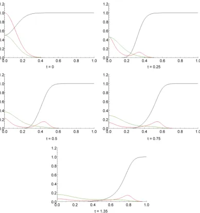
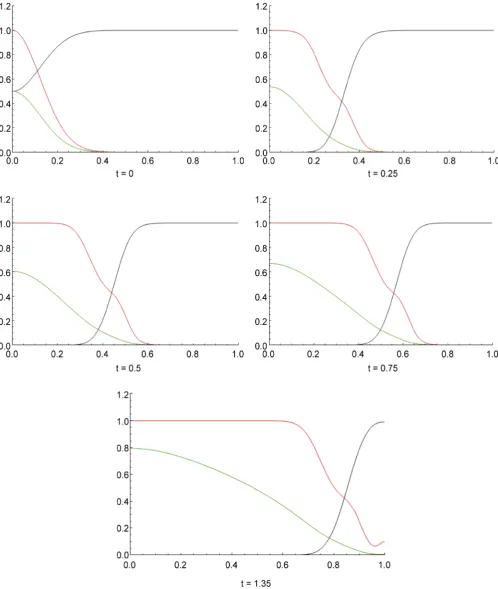
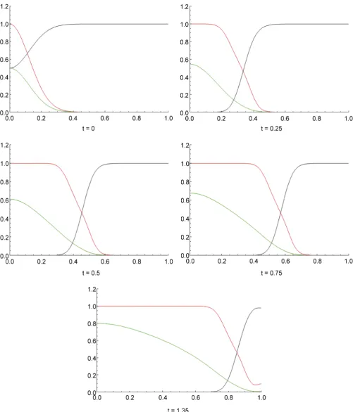
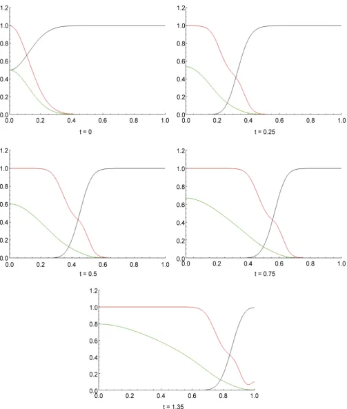
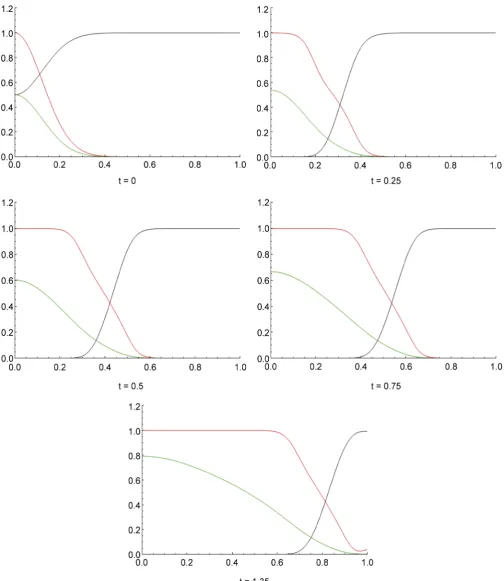
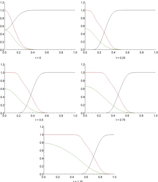
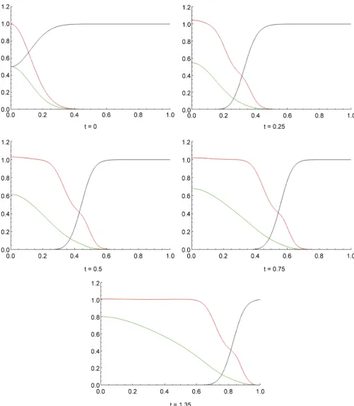
[image:8.595.161.551.217.632.2]µ = , µ =2 0 ~ 5, α =0.1, β =0.1 and xn =0 ~ 0.01 specified below. We will observe the time dependent relationship and interaction between tumour cells (Red line), the surrounding tissue (Black line) and degradation enzymes (Green line). In the graphs below a coordinate axis of the horizontal direction indicates the spatial position and vertical direction indicates the density or concentration of each component of the model.
Figure 1. Interactions between the tumour and the surrounding tissue without proliferation of tumour cell, migration, and ECM re-establishment: The parameter values dn = 0.001, dm = 0.001, γ = 0.02, η = 10, μ1 = 0,
μ2 = 0, α = 0 and β = 0.1, xn = 0. We can observe that MDEs degradates the surrounding tissue, and makes
Figure 2. Tumour cell proliferation, migration, and interactions between the tumour and the surrounding tissue without ECM re-establishment: The parameter values dn = 0.001, dm = 0.001, γ = 0.02, η = 10, μ1 = 5, μ2 = 0, α = 0.1 and β = 0.1, xn = 0. It is seen that
[image:9.595.49.548.72.662.2]Figure 3. Tumour cell proliferation, migration, without ECM re-establishment, and interactions between the tumour and the surround-ing tissue: The parameter values dn = 0.001, dm = 0.001, γ = 0.02, η = 10, μ1 = 10, μ2 = 0, α = 0.1 and β = 0.1, xn = 0. Increasing μ1 more, it is
Figure 4. Tumour cell proliferation, migration, ECM re-establishment, and interactions between the tumour and the surrounding tissue: The parameter values dn = 0.001, dm = 0.001, γ = 0.02, η = 10, μ1 = 5, μ2 = 0.001, α = 0.1 and β = 0.1, xn = 0. We take μ2 = 0.001 only and
Figure 5. Tumour cell proliferation, migration, ECM re-establishment, and interactions between the tumour and the surrounding tissue: The parameter values dn = 0.001, dm = 0.001, γ = 0.02, η = 10, μ1 = 5, μ2 = 1, α = 0.1 and β = 0.1, xn = 0. When taking μ2 = 0.001, compared
Figure 6. Tumour cell proliferation, migration, ECM re-establishment, and interactions between the tumour and the surrounding tissue: The parameter values dn = 0.001, dm = 0.001, γ = 0.02, η = 10, μ1 = 5, μ2 = 5, α = 0.1 and β = 0.1, xn = 0. Compared with Figure 4 and
Figure 7. Tumour cell proliferation, chemotaxis, migration, ECM re-establishment, and interactions between the tumour and the sur-rounding tissue: The parameter values dn = 0.001, dm = 0.001, γ = 0.02, η = 10, μ1 = 5, μ2 = 0, α = 0.1 and β = 0.1, xn = 0.01. By the effect of
chemotaxis (xn = 0.01), tumour cells are attracted by MDEs, the density is beyond 1 at t = 0.25 ~ 0.5, eventually it converges to 1 and after
[image:14.595.46.548.68.643.2]5. Conclusions
In order to obtain the global existence in time and asymptotic profile of solutions of a mathematical model of tumour invasion proposed by Chaplain and Lolas, we investi-gate nonlinear evolution equations with logistic term related to our mathematical mod-els as an initial Neumann-boundary value problem. We could show the global existence in time of rigorous mathematical solutions to the initial boundary value problem for the model in arbitrary space dimension by using the energy inequalities. Applying the result to our model we show global existence in time of mathematical solutions of the model.
By Figures 1-7, it is recognized that our rigorous mathematical result of the exis-tence and asymptotic behaviour of smooth solutions verifies our computer simulations and confirms the pattern form of each component of the model in the graphs respec-tively. Then we can gain the understanding of the process of tumour invasion more in details.
Acknowledgements
This work was supported in part by the Grants-in-Aid for Scientific Research (C) 19540200, 22540208, 25400148 and 16K05214 from Japan Society for the Promotion of Science.
References
[1] Chaplain, M.A.J. and Lolas, G. (2006) Mathematical Modeling of Cancer of Tissue: Dy-namic Heterogeneity. Networks and Heterogeneous Media, 1, 399-439.
http://dx.doi.org/10.3934/nhm.2006.1.399
[2] Anderson, A.R.A. and Chaplain, M.A.J. (2003) Mathematical Modelling of Tissue Invasion, In: Preziosi, L., Ed., Cancer Modelling and Simulation, Chapman Hall/CRC, 269-297. [3] Kubo, A. and Kimura, K. (2014) Mathematical Analysis of Tumour Invasion with
Prolifera-tion Model and SimulaProlifera-tions. WSEAS Transaction on Biology and Biomedicine, 11, 165- 173.
[4] Kubo, A. and Hoshino, H. (2015) Nonlinear Evolution Equation with Strong Dissipation and Proliferation, Current Trends in Analysis and Its Applications. Springer, Birkhauser, 233-241.
[5] Kubo, A. and Suzuki, T. (2004) Asymptotic Behavior of the Solution to a Parabolic ODE System Modeling Tumour Growth. Differential and Integral Equations, 17, 721-736. [6] Kubo, A., Suzuki, T. and Hoshino, H. (2005) Asymptotic Behavior of the Solution to a
Pa-rabolic ODE System. Mathematical Sciences and Applications, 22, 121-135.
[7] Kubo, A. and Suzuki, T. (2007) Mathematical Models of Tumour Angiogenesis. Journal of Computational and Applied Mathematics, 204, 48-55.
http://dx.doi.org/10.1016/j.cam.2006.04.027
[8] Kubo, A., Saito, N., Suzuki, T. and Hoshino, H. (2006) Mathematical Models of Tumour Angiogenesis and Simulations, Theory of Bio-Mathematics and Its Application. RIMS Ko-kyuroku, 1499, 135-146.
[9] Kubo, A. (2011) Nonlinear Evolution Equations Associated with Mathematical Models,
[10] Dionne, P. (1962) Sur les problèmes de Cauchy hyperboliques bien posés. Journal d'Analyse Mathematique, 10, 1-90.http://dx.doi.org/10.1007/BF02790303
[11] Andasari, V., Roper, R.T., Swat, M.H. and Chaplain, M.A.J. (2011) Integrating Intracellular Dynamics Using CompuCell3D and Bionetsolver: Applications to Multiscale Modelling of Cancer Cell Growth and Invasion. PLoS ONE, 7, e33726.
http://dx.doi.org/10.1371/journal.pone.0033726
[12] Anderson, A.R.A. and Chaplain, M.A.J. (1998) Continuous and Discrete Mathematical Models of Tumour-Induced Angiogenesis. Bulletin of Mathematical Biology, 60, 857-899.
http://dx.doi.org/10.1006/bulm.1998.0042
[13] Deakin, N.E. and Chaplain, M.A.J. (2013) Mathematical Modeling of Cancer Invasion: The Role of Membrane-Bound Matrix Metalloproteinases. Frontiers in Oncology, 3, 70.
http://dx.doi.org/10.3389/fonc.2013.00070
[14] Hatami, F. and Ghaemi, M.B. (2013) Numerical Solution of Model of Cancer Invasion with Tissue. Applied Mathematics, 4, 1050-1058. http://dx.doi.org/10.4236/am.2013.47143
[15] Kim, Y. and Othmer, H.G. (2013) A Hybrid Model of Tumor-Stromal Interactions in Breast Cancer. Bulletin of Mathematical Biology, 75, 1304-1350.
http://dx.doi.org/10.1007/s11538-012-9787-0
[16] Kolev, M. and Zubik-Kowal, B. (2011) Numerical Solutions for a Model of Tissue Invasion and Migration of Tumourcells. Computational and Mathematical Methods in Medicine, 2011, Article ID: 452320. http://dx.doi.org/10.1155/2011/452320
[17] Mahiddin, N. and Hashim, A. (2014) Approximate Analytical Solutions for Mathematical Model of Tumourinvasion and Metastasis Using Modified Adomian Decomposition and Homotopy Perturbation Methods. Journal of Applied Mathematics, 2014, Article ID: 654978. http://dx.doi.org/10.1155/2014/654978
[18] Märkl, C., Meral, G. and Surulescu, C. (2013) Mathematical Analysis and Numerical Simu-lations for a System Modeling Acid-Mediated Tumor Cell Invasion. International Journal of Analysis, 2013, Article ID: 878051.
[19] Orlando, P.A., Gatenby, R.A. and Brown, J.S. (2013) Tumor Evolution in Space: The Effects of Competition Colonization Tradeoffs on Tumor Invasion Dynamics. Frontiers in Oncol-ogy, 3, 45. http://dx.doi.org/10.3389/fonc.2013.00045
[20] Levine, H.A. and Sleeman, B.D. (1997) A System of Reaction and Diffusion Equations Arising in the Theory of Reinforced Random Walks. SIAM Journal on Applied Mathemat-ics, 57, 683-730. http://dx.doi.org/10.1137/S0036139995291106
[21] Othmer, H.G. and Stevens, A. (1997) Aggregation, Blowup, and Collapse: The ABCs of Taxis in Reinforced Random Walks. SIAM Journal on Applied Mathematics, 57, 1044- 1081. http://dx.doi.org/10.1137/S0036139995288976
[22] Chaplain, M.A.J., Lachowicz, M., Szymanska, Z. and Wrzosek, D. (2011) Mathematical Modeling of Cancer Invasion: The Importance of Cell-Cell Adhesion and Cell-Matrix Ad-hesion. Mathematical Models & Methods in Applied Sciences, 21, 719-743.
http://dx.doi.org/10.1142/S0218202511005192
[23] Sleeman, B.D. and Levine, H.A. (2001) Partial Differential Equations Chemotaxis and An-giogenesis. Mathematical Methods in the Applied Sciences, 24, 405-426.
http://dx.doi.org/10.1002/mma.212
Submit or recommend next manuscript to SCIRP and we will provide best service for you:
Accepting pre-submission inquiries through Email, Facebook, LinkedIn, Twitter, etc. A wide selection of journals (inclusive of 9 subjects, more than 200 journals)
Providing 24-hour high-quality service User-friendly online submission system Fair and swift peer-review system
Efficient typesetting and proofreading procedure
Display of the result of downloads and visits, as well as the number of cited articles Maximum dissemination of your research work