Document downloaded from:
This paper must be cited as:
The final publication is available at
http://dx.doi.org/10.1016/j.patrec.2010.12.002 http://hdl.handle.net/10251/37325
Villegas, M.; Paredes Palacios, R. (2011). Dimensionality reduction by minimizing nearest-neighbor classification error. Pattern Recognition Letters. 32(4):633-639.
Dimensionality Reduction by Minimizing
Nearest-Neighbor Classification Error
Mauricio Villegas1 and Roberto Paredes
Instituto Tecnol´ogico de Inform´atica, Universidad Polit´ecnica de Valencia,
Camino de Vera s/n, Edif. 8G Acc. B, 46022 Valencia (Spain). Tel: (+34) 963877069 - Fax: (+34) 963877239
mvillegas@ iti. upv. es,rparedes@ iti. upv. es
Abstract
There is a great interest in dimensionality reduction techniques for tackling the problem of high-dimensional pattern classification. This paper addresses the topic of supervised learning of a linear dimension reduction mapping suitable for classification problems. The proposed optimization procedure is based on minimizing an estimation of the nearest neighbor classifier error probability, and it learns a linear projection and a small set of prototypes that support the class boundaries. The learned classifier has the property of be-ing very computationally efficient, makbe-ing the classification much faster than state-of-the-art classifiers, such as SVMs, while having competitive recogni-tion accuracy. The approach has been assessed through a series of experi-ments, showing a uniformly good behavior, and competitive compared with some recently proposed supervised dimensionality reduction techniques.
Keywords:
Dimensionality Reduction, Pattern Recognition, Nearest-Neighbor Classifier
1. Introduction
Dimensionality reduction techniques play a very important role in pattern recognition tasks in which the feature vectors lay on a high-dimensional space. It is difficult to directly apply machine learning algorithms to this type of
tasks because of the so called curse of dimensionality. On the other hand, data visualization is usually needed in applications where an expert can derive useful knowledge from low-dimensional data representations.
Because of their simplicity and effectiveness, the two most popular di-mensionality reduction techniques are Principal Component Analysis (PCA) and Linear Discriminant Analysis (LDA) Fukunaga (1990), being the former unsupervised and the latter supervised. Among their limitations, both of these methods are linear and assume a Gaussian distribution of the data. Additionally, LDA has an upper limit of C−1 for the number of components after the mapping, being C the number of classes. To overcome these and other limitations, subsequent methods have been proposed, where the non-linear problem is commonly approached by extending the non-linear algorithms using the kernel trick Mika et al. (1999); Sch¨olkopf et al. (1999).
Methods based on finding the lower dimensional manifold in which the data lies are ISOMAP Tenenbaum et al. (2000) and Locally Linear Em-bedding (LLE) Roweis and Saul (2000); de Ridder et al. (2003), which are non-linear, and Locality Preserving Projections (LPP, SLPP) He and Niyogi (2004); Zheng et al. (2007), Linear Laplacian Discrimination (LLD) Zhao et al. (2007) and Locality Sensitive Discriminant Analysis (LSDA) Cai et al. (2007), which are linear. A work worth mentioning is Yan et al. (2007) in which the authors propose the Marginal Fisher Analysis (MFA) and a Graph Embedding Framework under which all of the methods mentioned so far can be viewed. From a different point of view, is worth mentioning the Self Orga-nizing Map (SOM) Kohonen (1982), an unsupervised neural network closely related to these techniques since it aims at producing a low-dimensional em-bedding of the data preserving the topological properties of the input space. In the present work, the dimensionality reduction mapping is learned by minimizing a Nearest-Neighbor (1-NN) classification error probability esti-mation. Therefore this work is related with other methods in which the op-timization is based on trying to minimize thek-NN classification error prob-ability, among them Nonparametric Discriminant Analysis (NDA) Bressan and Vitri`a (2003), Neighbourhood Component Analysis (NCA) Goldberger et al. (2005) and Large Margin Nearest Neighbour (LMNN) Weinberger et al. (2006) are worth mentioning.
In Villegas and Paredes (2008) we proposed a new algorithm that learns simultaneously a linear projection and a reduced set of prototypes. This pre-liminary work has some limitations. In the present paper we propose a new formulation of this approach which results in a more efficient implementation
of the algorithm. Additionally, the originally proposed approach learned an unrestricted projection matrix. In this paper, the method forces the projec-tion matrix to be orthonormal. Depending on the data set, this modificaprojec-tion can lead to better recognition accuracy as can be observed in the results presented.
An extensive experimentation comparing our approach with recently pro-posed linear supervised dimensionality reduction methods and Support Vec-tor Machines is carried out. The experimental results show that the proposed approach is clearly competitive both in classification accuracy and speed. Furthermore, we show that although the algorithm gives a complete 1-NN classifier, the learned subspace alone, which we refer to as LDPP*, is very competitive compared to state-of-the-art supervised dimensionality reduction techniques.
The remainder of the paper is organized as follows. Section 2 introduces the notation used throughout the paper. In section 3 the proposed dimen-sionality reduction approach is presented. Experimental results are presented in section 4. The final section draws the conclusions and directions for future research.
2. Preliminaries and Notation
Following common notation, column vectors will be denoted by lowercase bold letters. To denote row vectors, the transpose operator (T) will be used. Matrices will be denoted by uppercase bold letters and sets using uppercase calligraphic. Any other symbol which is not in bold font is either a scalar or a function.
Two representation spaces will be distinguished. The first one, which will be referred to as the original space, is the space where the objects of interest are originally represented. It is assumed that this is a D-dimensional real valued vector space, i.e., RD. The other representation space, which will be referred to as the target space, is the space in which the objects of interest are represented after the dimensionality reduction transformation has been applied. This space is assumed to be an E-dimensional real valued vector space, i.e., RE. Certainly, the dimensionality of the target space will be
always smaller than the dimensionality of the original space, that is E < D. In general, the dimensionality reduction transformation can be any func-tion, however the present work is only concerned with linear transformations which will be specified by a matrix B∈RD×E. For convenience, throughout
the paper, vectors in the original and the target spaces will be denoted with the same symbol, with the difference that vectors in the target space will have a tilde. Using this notation, a linear mapping from the original space to the target space is given by:
˜
x=BTx, x∈RD, x˜ ∈RE. (1) Some functions which will be used in this work are the following. The Heaviside step function centered at z = 1, is defined as:
step(z) =
0 if z <1
1 if z ≥1. (2)
As an approximation to the step function, the sigmoid function with slope
β, centered at z = 1 will be used. It is defined as:
Sβ(z) =
1
1 +eβ(1−z) . (3)
Note that if β is large, then Sβ(z) ≈step(z),∀z ∈ R, z 6= 1. The derivative
of the sigmoid function, also needed in this work, is given by S′ β(z) = d Sβ(z) dz = βeβ(1−z) (1 +eβ(1−z))2 . (4) S′
β(z) is a windowing function which is maximum for z = 1 and vanishes for |z −1| ≫ 0. If β is large, then S′
β(z) approaches the Dirac delta function,
conversely, if β is small, then S′
β(z) is approximately constant for a wide
range of values of z.
3. Learning Discriminative Projections and Prototypes
The objective of the algorithm is to learn a projection base B ∈ RD×E by minimizing the error rate of the Nearest-Neighbor (1-NN) classifier on a training set X = {x1, . . . ,xN} ⊂ RD whose samples belong to one of C
classes. A method for estimating the error rate is therefore required. A pop-ular method of estimation of the error is Leave-One-Out (LOO) Paredes and Vidal (2006). However, the LOO estimation for a 1-NN classifier has the problem that vectors tend to pair up, producing complex decision bound-aries that do not generalize well to unseen data and giving an optimistic
estimate of the error rate. To overcome this problem, an alternative way of estimating the error rate is to define a new set of class labeled prototypes P ={p1, . . . ,pM} ⊂ RD, different from and much smaller than the training set X, and with at least one prototype per class, i.e. P 6⊂ X, C ≤M ≪N. These will be the reference prototypes used to estimate the 1-NN classifica-tion error probability. For simplicity, all of the classes will have the same number of prototypes, i.e. Mc =M/C.
An approximation of the 1-NN error rate of the training setX projected on the target space using the reference prototypes P can be written as:
JX(B,P) = 1 N X ∀x∈X Sβ(Rx), (5) where Rx = d(˜x,p˜∈) d(˜x,p˜∈/) . (6)
As it has been pointed out in Paredes and Vidal (2006), the sigmoid approx-imation with an adequate β may be preferable than the exact step function. This is because the contribution of each sample to the goal function JX
be-comes more or less important depending on the quotient of the distances. This way the sigmoid approximation has a smoothing effect capable of ig-noring clear outliers in the data and not learning from correctly classified samples which are far from the decision boundary.
From equation (5) the following expressions can be derived: ∇BJX = 1 N X ∀x∈X S′ β(Rx)Rx d(˜x,p˜∈) ∇Bd(˜x,p˜∈) − 1 N X ∀x∈X S′ β(Rx)Rx d(˜x,p˜∈/) ∇Bd(˜x,p˜∈/), (7) ∇pmJX = 1 N X ∀x∈X: ˜ pm=˜p∈ S′ β(Rx)Rx d(˜x,p˜∈) ∇pm d(˜x,p˜∈) − 1 N X ∀x∈X: ˜ pm=˜p∈/ S′ β(Rx)Rx d(˜x,p˜∈/) ∇pmd(˜x,p˜∈/), (8)
where the sub-index m, indicates that it is the m-th prototype of P. If the squared Euclidean distance is used, the corresponding gradients with respect to the parameters are:
∇Bd(˜x,p) = 2(x˜ −p)(˜x−p)˜ T , (9) ∇pd(˜x,p) =˜ −2B(˜x−p)˜ . (10)
In order to simplify the subsequent equations, the factors in (7) and (8) will be denoted by: F∈ = S′ β(Rx)Rx d(˜x,p˜∈) , and F∈/ = S′ β(Rx)Rx d(˜x,p˜∈/) . (11)
Looking at the gradient equations the update procedure can be summa-rized as follows. In every iteration, each vector x ∈ X is visited and the projection base and the prototype positions are updated. The matrix B is modified so that it projects the vector x closer to its same-class nearest prototype in the target space, ˜p∈. Similarly, B is also modified so that it
projects the vector x farther away from its different-class nearest prototype ˜
p∈/. Simultaneously, the nearest prototypes in the original space, p∈ and p∈/, are modified so that their projections are, respectively, moved towards and away from ˜x.
3.1. The LDPP Algorithm
An efficient implementation of the algorithm can be achieved if the gradi-ents with respect to B and P are simple linear combinations of the training setX and the prototypes P. This property holds for the euclidean distance, and it may hold for other distances as well (although not for all possible distances).
Let the training set and the prototypes be arranged into matrices X ∈ RD×N andP ∈RD×M, with each column having a vector of the set. Then the gradients can be expressed as a function of some factor matrices G∈RE×N and H ∈RE×M as:
∇BJX =XGT+P HT , (12)
In the particular case of the Euclidean distance, the n-th and m-th columns of the factor matrices G and H are:
gn= 2 NF∈n(˜xn−p˜∈n) − 2 NF∈/n(˜xn−p˜∈/n) , (14) hm =− 2 N X ∀x∈X: ˜ pm=˜p∈ F∈(˜x−p˜∈) + 2 N X ∀x∈X: ˜ pm=˜p∈/ F∈/(˜x−p˜∈/) . (15)
Finally, the optimization is performed using the corresponding gradient de-scent update equations:
B(t+1) =B(t)−γ∇BJX , (16)
P(t+1) =P(t)−η∇P JX . (17)
Up to this point the projection baseBis not an orthonormal basis. A simple approach we propose to ensure an orthonormal projection is to perform a Gram-Schmidt process after each gradient update.
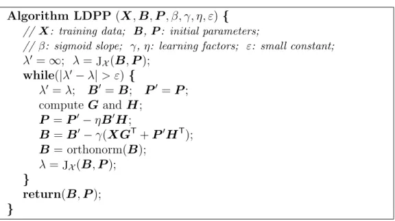
The resulting optimization procedure is summarized in the algorithm
Learning Discriminant Projections and Prototypes (LDPP)2, presented in
figure 1.
The time complexity of the algorithm isO(DEN) per iteration, which is considerably more efficient than the original proposal Villegas and Paredes (2008). Still, this is the complexity of the learning stage, which can be performed in a powerful server. On the other hand, the complexity for the classification phase is O(DE +EM), which is considerably fast compared to other classification approaches which normally are O(DE +EN) being
M ≪N.
2A Matlab/Octave implementation is available in
Algorithm LDPP(X,B,P, β, γ, η, ε) {
// X: training data; B, P: initial parameters;
// β: sigmoid slope; γ, η: learning factors; ε: small constant;
λ′ =∞; λ= JX(B,P); while(|λ′ −λ|> ε){ λ′ =λ; B′ =B; P′ =P; compute G and H; P =P′−ηB′H; B=B′−γ(XGT+P′ HT); B= orthonorm(B); λ= JX(B,P); } return(B,P); }
Figure 1: Learning discriminant projections and prototypes (LDPP) algorithm.
3.2. Discussion
The proposed approach is also related to the family of pattern recog-nition algorithms based on gradient descent optimization, in particular, the neural networks algorithms Bishop (1995) such as the Multi Layer Perceptron (MLP) which uses the Backpropagation algorithm Rumelhart et al. (1986) for learning and the SOM neural network mentioned in the introduction. The MLP and the proposed algorithm both use a sigmoid function, the MLP uses it for handling non-linear problems while our algorithm introduces it to obtain a suitable approximation to the 1-NN classification error rate. An-other similarity is that the number of hidden neurons and the number of prototypes of the proposed method defines the structural complexity and its representation capability.
In general all the methods based on gradient descent optimization have the same properties. These methods are easy to implement, they only require to optimize a differentiable function and are easily tuned by means of con-trolling the learning factor. On the other hand, they may generally converge to any local minimum on the target function surface. The local minimum reached will depend on the initialization of the algorithm. In our case using PCA andk-means for initialization, generally leads to a fast convergence and very good results as the experiments show.
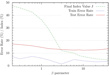
The convergence of the algorithm is very stable for a wide range of values of the parameter β of the sigmoid function, see figure 3. For low values of
β the goal function starts and stays close to 0.5 for all the parameter space (B,P). In this case the convergence becomes very slow and is hard to judge when to stop iterating. Moreover low values of β entail a significant diver-gence between the goal function and the 1-NN error rate. This diverdiver-gence is reduced using high values of β but then it becomes more likely that the algo-rithm converges to a local minima due to the roughness of the goal function along the parameter space. Empirically it has been observed that a value of β = 10 provides a good balance, because it is a point in which the goal function is a good estimator of the error rate and the algorithm does not seem to get stuck in local minima.
4. Experiments
The proposed approach has been assessed with different problems. First, some results are presented on synthetic data to illustrate the behavior of the algorithm. After this, we show classification results for several data sets with a great variety in size of the corpus, number of classes, and dimensionality. Followed by this, some results are presented using a high-dimensional data, for which the algorithm is mainly intended.
The proposed approach was compared with similar techniques, i.e. linear and supervised, namely LDA, MFA, LSDA, SLPP, NDA, NCA and LMNN all of them with and without a PCA preprocessing. For LDA our own im-plementation was used, however for the rest, we used freely available imple-mentations from the authors of Cai et al. (2007); Bressan and Vitri`a (2003); Weinberger et al. (2006); Fowlkes et al. (2007). For each of the baseline methods, the corresponding algorithm parameters were properly adjusted, and only the best result obtained in each case is shown. A k-NN classifier was used for all these dimensionality reduction techniques. The k parameter of the classifier was also varied and the best result is the one presented.
The initialization used for the LDPP algorithm in all of the experiments was a per class k-means for the prototypes P and PCA for the projection base B. It has been observed that this simple initialization provides good convergence behavior and recognition results. For LDPP, the training data was previously normalized so that each component had a zero mean and unit variance. Furthermore, the learned projection bases have been restricted to being orthonormal. It was observed that these modifications helped to make
the learning factors more stable across different data sets, and thus making more narrow the range of values of the parameters to explore. For all of the experiments, the results are for β = 10. Aditionally in the high-dimensional data sets, different values ofβ are used to show the effect that this parameter produces on the results.
There are two different results for LDPP, either using the learned proto-types and a 1-NN classifier shown as plain LDPP, or using the whole training set and a k-NN classifier, shown as LDPP*.
The proposed algorithm condenses the training set into a very compact classifier, and this added to the fact that it is linear, makes the classifier extremely fast, in the results we have also included what we call thespeedup. This is a measure of how many times faster is the testing phase of the method compared to what it takes using ak-NN classifier in the original space. This relative measure has been estimated using the time complexity of the algo-rithms.
Although the Support Vector Machine (SVM) is not a dimensionality reduction method, it can be considered the state-of-the-art in pattern clas-sification, for this reason in some of the experiments a comparison was also made with SVM. For this, we used the multi-class LIBSVM Chang and Lin (2001) implementation. In each experiment, the linear, polynomial and RBF kernels were tried, and for each one, the penalty and kernel parameters were varied to obtain the best result.
4.1. Synthetic Data
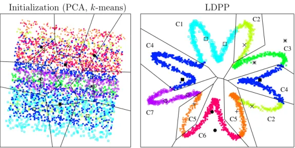
Figure 2 presents the 2-D visualization of a 7 class 6-dimensional syn-thetic data set. Three of the dimensions conform a 3-dimensional helix with the classes distributed along this helix, generated using the tool mentioned in L.J.P. van der Maaten (2007). The other 3 additional dimensions are random noise. Some of the classes are multi-modal and therefore the result obtained by classical techniques such as LDA gives an overlap between the classes. The figure first shows the initialization of the algorithm which was PCA and two prototypes per class obtained by k-means. The second plot shows the result obtained after LDPP learning.
As can be observed in the figure, the projection learned completely re-moves the noise and the reference prototypes are positioned so that they classify very well the data. Although this is a very ideal synthetic data set, it illustrates how the algorithm works. If we would have chosen only one
Initialization (PCA, k-means) LDPP C1 C2 C2 C3 C4 C4 C5 C5 C6 C7
Figure 2: 2-D visualization of a 3-D synthetic helix with 3 additional dimensions of random noise. The graphs include the prototypes (big points in black), the corresponding voronoi diagram and the training data (small points in color). At the left is the initialization (PCA
andk-means) and at the right, the final result after LDPP learning.
prototype per class it would have been impossible for the prototypes to clas-sify well the data. For a real data set the number of prototypes needs to be varied and the best result will be the one that gives a low error rate with the least number of prototypes. The number of prototypes is desired to be low because it defines structural complexity of the recognizer and this affects the generalization capabilities to unseen samples.
4.2. UCI and Statlog Corpora
Although the proposed approach has been developed for high-dimensional tasks, it is still a classifier learning technique that works with an arbitrary vector valued classification problem. In this section we present some results for several data sets form the UCI Machine Learning Repository Asuncion and Newman (2007), most of which are low-dimensional. As can be observed in table 1, the selected data sets have a wide variety in the number of samples, number of classes and feature dimensionality.
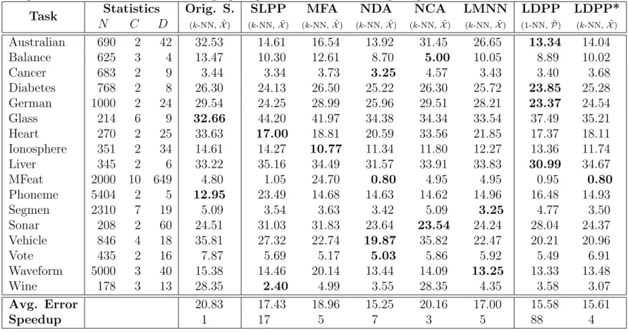
Table 1: Error rates (in %) for several data sets and different dimensionality reduction techniques. The last two rows are the
average classification error rate and the average speedup relative tok-NN in the original space.
Task Statistics Orig. S. SLPP MFA NDA NCA LMNN LDPP LDPP*
N C D (k-NN, ˜X) (k-NN, ˜X) (k-NN, ˜X) (k-NN, ˜X) (k-NN, ˜X) (k-NN, ˜X) (1-NN, ˜P) (k-NN, ˜X) Australian 690 2 42 32.53 14.61 16.54 13.92 31.45 26.65 13.34 14.04 Balance 625 3 4 13.47 10.30 12.61 8.70 5.00 10.05 8.89 10.02 Cancer 683 2 9 3.44 3.34 3.73 3.25 4.57 3.43 3.40 3.68 Diabetes 768 2 8 26.30 24.13 26.50 25.22 26.30 25.72 23.85 25.28 German 1000 2 24 29.54 24.25 28.99 25.96 29.51 28.21 23.37 24.54 Glass 214 6 9 32.66 44.20 41.97 34.38 34.34 33.54 37.49 35.21 Heart 270 2 25 33.63 17.00 18.81 20.59 33.56 21.85 17.37 18.11 Ionosphere 351 2 34 14.61 14.27 10.77 11.34 11.80 12.27 13.36 11.74 Liver 345 2 6 33.22 35.16 34.49 31.57 33.91 33.83 30.99 34.67 MFeat 2000 10 649 4.80 1.05 24.70 0.80 4.95 4.95 0.95 0.80 Phoneme 5404 2 5 12.95 23.49 14.68 14.63 14.62 14.96 16.48 14.93 Segmen 2310 7 19 5.09 3.54 3.63 3.42 5.09 3.25 4.77 3.50 Sonar 208 2 60 24.51 31.03 31.83 23.64 23.54 24.24 28.04 24.37 Vehicle 846 4 18 35.81 27.32 22.74 19.87 35.82 22.47 20.21 20.96 Vote 435 2 16 7.87 5.69 5.17 5.03 5.86 5.92 5.49 6.91 Waveform 5000 3 40 15.38 14.46 20.14 13.44 14.09 13.25 13.33 13.48 Wine 178 3 13 28.35 2.40 4.99 3.55 28.35 4.35 3.58 3.07 Avg. Error 20.83 17.43 18.96 15.25 20.16 17.00 15.58 15.61 Speedup 1 17 5 7 3 5 88 4 12
To estimate the error rates, anS-fold cross-validation procedure was em-ployed, using one set for test, another one for development and the rest for training. The estimation of the error rate is the error of the test set for the parameters which gave the lowest error rate in the development set. This way the estimated error rates also take into account the generalization to unseen data.
Table 1 shows the results obtained by a 20 time repeated 5-fold cross-validation, as explained previously. The last two rows of the table are a summary of the results for all of the data sets. First, the average classi-fication error indicates recognition performance in comparison to the other techniques. And second, the speedup indicates the efficiency of the classifier in the testing phase, as was explained in the beginning of the section. For LDPP, depending on the data set, using the learned prototypes instead of the whole training set, does or does not improve the recognition. Although on average it is better to use the learned prototypes. In comparison with the baseline techniques, on average the proposed approach performs very well, having a lower error rate than all of the techniques except for NDA. Remark that LDPP is much faster than the other techniques in the testing phase. In particular, LDPP is more than 10 times faster than NDA for a very similar average error rate.
4.3. High-Dimensional Data Sets
As representatives of high-dimensional problems, due to their current high interest, we have considered two face image analysis tasks, gender and emotion recognition. Gender recognition is a two class problem, ei-ther male or female, which makes it interesting in this context since sev-eral supervised dimensionality reduction techniques in the literature have
C − 1 as an upper limit for the target space dimensionality. For these methods the target dimensionality is at most one, a restriction that the proposed approach does not have. The gender data set is the same as the one described in Villegas and Paredes (2008), composed of 1892 images, half males and half females, obtained from the following databases: AR Face Database Martinez and Benavente (1998), BANCA Database Bailly-Bailli´ere et al. (2003), Caltech Frontal Face Database Weber, Essex Collec-tion of Facial Images Spacek, FERET Database Phillips et al. (2000), FRGC Database Phillips et al. (2005), Georgia Tech Face Database Nefian and the XM2VTS Database Messer et al. (1999). The images were converted to
0 10 20 30 40 50 1 10 E rr or R at e (% ) / In d ex (% ) βparemeter
Final Index Value J Train Error Rate Test Error Rate
Figure 3: Graph illustrating the relationship of the β parameter with the recognition
performance and goal function. This is an average of the 5-fold cross-validation for both the gender and emotion data sets.
gray-scale, cropped to a size of 32×40 and histogram equalized3.
In contrast, the emotion recognition task considered is a seven class prob-lem, the six basic emotions Donato et al. (Oct 1999) and neutral face. The images were extracted from the Cohn-Kanade video database Kanade et al. (2000). Only 348 sequences were used, all of which the emotion labels are publicly available Buenaposada et al. (2008). Two images were used per se-quence, the first frame, which are neutral expressions, and the last frame, which is the apex of the corresponding emotion. As can be observed, the data set is not balanced. The images were converted to gray-scale, cropped to a size of 32×32 and histogram equalized2.
Figure 3 shows the relationship that the β parameter has on the recog-nition performance. As can be observed the performance does not change much, although a value of β = 10 seems to be the best one. A β = 10 has worked well for all of the data sets we have tried.
A single 5-fold cross-validation was employed to estimate the results. The
3Data sets available in
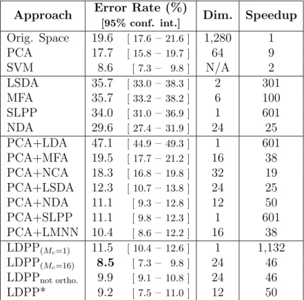
Table 2: Face gender recognition results for different dimensionality reduction techniques.
Approach Error Rate (%) Dim. Speedup
[95% conf. int.] Orig. Space 19.6 [ 17.6 –21.6 ] 1,280 1 PCA 17.7 [ 15.8 –19.7 ] 64 9 SVM 8.6 [ 7.3 – 9.8 ] N/A 2 LSDA 35.7 [ 33.0 –38.3 ] 2 301 MFA 35.7 [ 33.2 –38.2 ] 6 100 SLPP 34.0 [ 31.0 –36.9 ] 1 601 NDA 29.6 [ 27.4 –31.9 ] 24 25 PCA+LDA 47.1 [ 44.9 –49.3 ] 1 601 PCA+MFA 19.5 [ 17.7 –21.2 ] 16 38 PCA+NCA 18.3 [ 16.8 –19.8 ] 32 19 PCA+LSDA 12.3 [ 10.7 –13.8 ] 24 25 PCA+NDA 11.1 [ 9.3 –12.8 ] 12 50 PCA+SLPP 11.1 [ 9.8 –12.3 ] 1 601 PCA+LMNN 10.4 [ 8.6 –12.2 ] 16 38 LDPP(Mc=1) 11.5 [ 10.4 –12.6 ] 1 1,132 LDPP(Mc=16) 8.5 [ 7.3 – 9.8 ] 24 46 LDPPnot ortho. 9.9 [ 9.1 –10.8 ] 24 46 LDPP* 9.2 [ 7.5 –11.0 ] 12 50
results are presented in tables 2 and 3, for gender and emotion respectively. For LDPP the target space dimensionality was varied logarithmically between 1 and 48 and the number of prototypes per class was varied between 1 and 24 also logarithmically.
For both data sets the best result is presented with or without the proto-types, LDPP and LDPP* respectively. For gender also the result is presented when reducing to only one dimension, so that it can be compared with the other techniques that have such a extreme constraint. As can be observed in the tables, for both problems LDPP gives very competitive error rates. For gender, the best result is statistically significantly better than all the base-line techniques, except for SVM. However LDPP still gives a much faster classifier than SVM. In the emotion task LDPP also performs very well. Al-though the best target space dimensionality resulted to be higher than most of the baseline techniques. The tables also include the result when LDPP
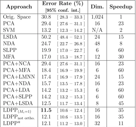
Table 3: Face emotion recognition results on the Cohn-Kanade database for different dimensionality reduction techniques.
Approach Error Rate (%) Dim. Speedup
[95% conf. int.] Orig. Space 30.8 [ 28.3– 33.3 ] 1,024 1 PCA 29.4 [ 27.6– 31.1 ] 16 23 SVM 13.2 [ 12.3– 14.2 ] N/A 2 LSDA 50.2 [ 48.4– 52.1 ] 24 15 NDA 24.7 [ 22.7– 26.8 ] 48 8 SLPP 19.9 [ 17.0– 22.7 ] 6 60 MFA 17.0 [ 15.3– 18.7 ] 12 30 PCA+NCA 29.4 [ 27.6– 31.1 ] 16 23 PCA+MFA 18.4 [ 16.9– 19.9 ] 6 60 PCA+LMNN 17.4 [ 16.9– 17.9 ] 24 15 PCA+NDA 15.7 [ 13.5– 17.8 ] 16 23 PCA+LDA 14.2 [ 13.2– 15.3 ] 6 60 PCA+SLPP 14.2 [ 13.2– 15.3 ] 6 60 PCA+LSDA 12.5 [ 11.7– 13.4 ] 8 45 LDPP(Mc=1) 11.5 [ 10.6– 12.4 ] 16 35 LDPPnot ortho. 12.1 [ 10.6– 13.5 ] 16 35 LDPP* 12.1 [ 11.2– 13.0 ] 32 11
does not force B to be orthonormal, and in both experiments giving worse performance. This suggests that depending on the problem, the orthonor-malization is capable of improving the recognition results.
In general the baseline techniques tend to work bad handling the orig-inal high dimensional space, making these techniques inadequate for high-dimensional problems. On the other hand, LDPP is capable of handling the data in the original space. In general the baseline techniques work better using a previous PCA. Notice the relative bad results obtained by NDA in this high-dimensional scenario and even when is combined with PCA is still far from the best result obtained by our LDPP.
In the original space LDA is unable to give a result due singularity prob-lems. Moreover with such a high dimensionality both NCA and LMNN are extremely slow, thus we were unable to compute those results.
5. Conclusions
In this paper we have presented the LDPP algorithm. This algorithm learns simultaneously a linear projection and a reduced set of prototypes that define adequately the class distributions on the target space. In the present work we have introduced a more elegant formulation for LDPP which leads to a more efficient and easily parallelizable implementation. Furthermore, the approach has been modified to ensure that the resulting projection ma-trix is orthonormal. Experimental results confirm that this modification can improve the recognition results.
From the experiments we can conclude that the LDPP approach behaves considerably well for a wide range of problems. It achieves very competitive results for supervised dimensionality reduction, comparable to state-of-the-art techniques. The results on high-dimensional problems show that unlike other techniques, LDPP obtains competitive recognition performacen when applied to the original feature space and without having to resort to a PCA preprocessing. This has the advantage that no information is ignored during the discriminative learning. On the other hand, the technique additionally learns a small set of prototypes optimized for 1-NN classification, which in conjunction to the linear dimensionality reduction, gives an extremely fast classifier when compared with other classification approaches. Finally, the results show that there are problems where ignoring the learned prototypes, referred to as LDPP*, and using an alternative classifier may lead to better recognition accuracy. This shows that the projection base alone is quite discriminative and the prototypes are simply a way of estimating the error rate to be able to minimize it.
Future research will be focused on the use of different distances on the LDPP. Moreover distances for which the derivatives with respect to the model parameters can not be obtained could be applied, thus some approximation to such derivatives have to be used. On the other hand, alternative goal functions could be proposed to be optimized. For some problems the error rate minimization has no sense, and other goal functions would be more adequate, for instance one related to the area under the ROC curve Villegas and Paredes (2009). Also it would be interesting to extend LDPP to be semi-supervised to be used in problems where it is expensive to label all of the training data. As a final direction of future research, it is worth mentioning that in this moment there is a great interest in classification problems where there are millions of training samples available. The proposed approach does
not scale to corpora of this magnitude, therefore future work could be focused on this direction as well.
References
Asuncion, A., Newman, D., 2007. UCI machine learning repository. http://www.ics.uci.edu/ mlearn/MLRepository.html.
Bailly-Bailli´ere, E., Bengio, S., Bimbot, F., Hamouz, M., Kittler, J., Mari´ethoz, J., Matas, J., Messer, K., Popovici, V., Por´ee, F., Ru´ız, B., Thiran, J.P., 2003. The BANCA database and evaluation protocol, in: AVBPA, pp. 625–638.
Bishop, C.M., 1995. Neural Networks for Pattern Recognition. Oxford Uni-versity Press.
Bressan, M., Vitri`a, J., 2003. Nonparametric discriminant analysis and near-est neighbor classification. Pattern Recognition Letters 24, 2743–2749. Buenaposada, J.M., Mu˜noz, E., Baumela, L., 2008. Recognising facial
ex-pressions in video sequences. Pattern Anal. Appl. 11, 101–116.
Cai, D., He, X., Zhou, K., Han, J., Bao, H., 2007. Locality sensitive discrim-inant analysis, in: IJCAI, pp. 708–713.
Chang, C.C., Lin, C.J., 2001. LIBSVM: a library for support vector machines. Software available at http://www.csie.ntu.edu.tw/~cjlin/libsvm. Donato, G., Bartlett, M., Hager, J., Ekman, P., Sejnowski, T., Oct 1999.
Classifying facial actions. Transactions on Pattern Analysis and Machine Intelligence 21, 974–989.
Fowlkes, C.C., Martin, D.R., Malik, J., 2007. Local figure-ground cues are valid for natural images. Journal of Vision 7. http://www.
journalofvision.org/content/7/8/2.full.pdf+html.
Fukunaga, K., 1990. Introduction to Statistical Pattern Recognition. Aca-demic Press. 2 edition.
Goldberger, J., Roweis, S., Hinton, G., Salakhutdinov, R., 2005. Neighbour-hood components analysis, in: Saul, L.K., Weiss, Y., Bottou, L. (Eds.), Advances in Neural Information Processing Systems 17. MIT Press, Cam-bridge, MA, pp. 513–520.
He, X., Niyogi, P., 2004. Locality preserving projections, in: Thrun, S., Saul, L., Sch¨olkopf, B. (Eds.), Advances in Neural Information Processing Systems 16. MIT Press, Cambridge, MA.
Kanade, T., Tian, Y., Cohn, J.F., 2000. Comprehensive database for facial expression analysis, in: FG ’00: Proceedings of the Fourth IEEE Interna-tional Conference on Automatic Face and Gesture Recognition 2000, IEEE Computer Society, Washington, DC, USA. p. 46.
Kohonen, T., 1982. Self-organized formation of topologically correct feature maps. Biological Cybernetics 43, 59–69.
L.J.P. van der Maaten, 2007. An Introduction to Dimensionality Reduction Using Matlab. Technical Report MICC 07-07. Maastricht University. Martinez, A., Benavente, R., 1998. The AR face database. CVC Technical
Report #24.
Messer, K., Matas, J., Kittler, J., Luettin, J., Maitre, G., 1999. XM2VTSDB: The extended M2VTS database, in: Chellapa, R. (Ed.), Second Interna-tional Conference on Audio and Video-based Biometric Person Authenti-cation, University of Maryland, Washington, USA. pp. 72–77.
Mika, S., R¨atsch, G., Weston, J., Sch¨olkopf, B., M¨uller, K.R., 1999. Fisher discriminant analysis with kernels, in: Hu, Y.H., Larsen, J., Wilson, E., Douglas, S. (Eds.), Neural Networks for Signal Processing IX, IEEE. pp. 41–48.
Nefian, A.V., . Georgia tech face database.
http://www.anefian.com/face reco.htm.
Paredes, R., Vidal, E., 2006. Learning weighted metrics to minimize nearest-neighbor classification error. Pattern Analysis and Machine Intelligence, IEEE Transactions on 28, 1100–1110.
Phillips, P.J., Flynn, P.J., Scruggs, T., Bowyer, K.W., Chang, J., Hoffman, K., Marques, J., Min, J., Worek, W., 2005. Overview of the face recog-nition grand challenge, in: CVPR ’05: Proceedings of the 2005 IEEE Computer Society Conference on Computer Vision and Pattern Recogni-tion (CVPR’05) - Volume 1, IEEE Computer Society, Washington, DC, USA. pp. 947–954.
Phillips, P.J., Moon, H., Rizvi, S.A., Rauss, P.J., 2000. The FERET evalu-ation methodology for face-recognition algorithms. IEEE Transactions on Pattern Analysis and Machine Intelligence 22, 1090–1104.
de Ridder, D., Kouropteva, O., Okun, O., Pietik¨ainen, M., Duin, R.P.W., 2003. Supervised locally linear embedding, in: ICANN, pp. 333–341. Roweis, S.T., Saul, L.K., 2000. Nonlinear dimensionality reduction by locally
linear embedding. Science 290, 2323–2326.
Rumelhart, D.E., Hinton, G.E., Williams, R.J., 1986. Learning internal rep-resentations by error propagation, in: Rumelhart, D.E., McClelland, J.L. (Eds.), Parallel Distributed Processing: Explorations in the Microstruc-ture of Cognition. volume 1, pp. 318–362.
Sch¨olkopf, B., Smola, A.J., M¨uller, K.R., 1999. Kernel principal component analysis. Advances in kernel methods: support vector learning , 327–352.
Spacek, L., . Essex collection of facial images.
http://cswww.essex.ac.uk/mv/allfaces/index.html.
Tenenbaum, J.B., de Silva, V., , Langford, J.C., 2000. A global geometric framework for nonlinear dimensionality reduction. Science 290, 2319–2323. Villegas, M., Paredes, R., 2008. Simultaneous learning of a discriminative projection and prototypes for nearest-neighbor classification. Computer Vision and Pattern Recognition, 2008. CVPR 2008. IEEE Conference on , 1–8.
Villegas, M., Paredes, R., 2009. Score Fusion by Maximizing the Area Under the ROC Curve, in: 4th Iberian Conference on Pattern Recognition and Image Analysis. Springer, P´ovoa de Varzim, (Portugal). volume 5524 of
Weber, M., . Caltech frontal face database. http://www.vision.caltech.edu/html-files/archive.html.
Weinberger, K.Q., Blitzer, J., Saul, L.K., 2006. Distance metric learning for large margin nearest neighbor classification, in: In NIPS, pp. 1473–1480. Yan, S., Xu, D., Zhang, B., Zhang, H.J., Yang, Q., Lin, S., 2007. Graph
embedding and extensions: A general framework for dimensionality reduc-tion. Pattern Analysis and Machine Intelligence, IEEE Transactions on 29, 40–51.
Zhao, D., Lin, Z., Xiao, R., Tang, X., 2007. Linear laplacian discrimination for feature extraction, in: CVPR07, pp. 1–7.
Zheng, Z., Yang, F., Tan, W., Jia, J., Yang, J., 2007. Gabor feature-based face recognition using supervised locality preserving projection. Signal Processing 87, 2473 – 2483. Special Section: Total Least Squares and Errors-in-Variables Modeling.