1
Exploitation of Pairwise Class Distances for
Or-dinal Classification
J. S´anchez-Monedero
1
, Pedro A. Guti´errez
1
, Peter Ti ˇno
2
, C.
Herv´as-Mart´ınez
1
1Department of Computer Science and Numerical Analysis, University of C´ordoba,
C´ordoba 14071, Spain.
2School of Computer Science, The University of Birmingham, Birmingham B15 2TT,
United Kingdom.
Keywords:ordinal classification, ordinal regression, support vector machines, thresh-old model, latent variable
Abstract
Ordinal classification refers to classification problems in which the classes have a natu-ral order imposed on them because of the nature of the concept studied. Some ordinal classification approaches perform a projection from the input space to 1-dimensional
(latent) space that is partitioned into a sequence of intervals (one for each class). Class identity of a novel input pattern is then decided based on the interval its projection falls into. This projection is trained only indirectly as part of the overall model fitting. As with any latent model fitting, direct construction hints one may have about the desired form of the latent model can prove very useful for obtaining high quality models. The key idea of this paper is to construct such a projection model directly, using insights about the class distribution obtained from pairwise distance calculations. The proposed approach is extensively evaluated with eight nominal and ordinal classifiers methods, ten real world ordinal classification datasets, and four different performance measures. The new methodology obtained the best results in average ranking when considering three of the performance metrics, although significant differences are found only for some of the methods. Also, after observing other methods internal behaviour in the latent space, we conclude that the internal projection do not fully reflect the intra-class behaviour of the patterns. Our method is intrinsically simple, intuitive and easily un-derstandable, yet, highly competitive with state-of-the-art approaches to ordinal classi-fication.
1
Introduction
Ordinal classification or ordinal regression is a supervised learning problem of predict-ing categories that have an ordered arrangement. When the problem is really exhibitpredict-ing an ordinal nature, it is expected that this order is also present in the data input space (H¨uhn and H¨ullermeier, 2008). The samples are labelled by a set of ranks with an
ordering amongst the categories. In contrast to nominal classification, there is an or-dinal relationship throughout the categories and it is different from regression in that the number of ranks is finite and exact amounts of difference between ranks are not de-fined. In this way, ordinal classification lies somewhere between nominal classification and regression.
Ordinal regression should not be confused with sorting or ranking. Sorting is related to ranking all samples in the test set, with a total order. Ranking is related to ranking with a relative order of samples and a limited number of ranks. Of course, ordinal regression can be used to rank samples, but its objective is to obtain a good accuracy, and, at the same time, a good ranking.
Ordinal classification problems are important, since they are common in our ev-eryday life where many problems require classification of items into naturally ordered classes. Examples of these problems are the teaching assistant evaluation (Lim et al., 2000), car insurance risk rating (Kibler et al., 1989), pasture production (Barker, 1995), preference learning (Arens, 2010), breast cancer conservative treatment (Cardoso et al., 2005), wind forescasting (Guti´errez et al., 2013) or credit rating (Kim and Ahn, 2012). Variety of approaches have been proposed for ordinal classification. For exam-ple, Raykar et al. (2008) learns ranking functions in the context of ordinal regression and collaborative filtering datasets. Kramer et al. (2010) map the ordinal scale by as-signing numerical values and then apply a regression tree model. The main problem with this simple approach is the assignment of a numerical value corresponding to each class, without a principled way of deciding the true metric distances between the ordi-nal scales. Also, representing all patterns in a class by the same value may not reflect
the relationships among the patterns in a natural way. In this paper we propose that the numerical values associated with different patterns may differ (even within the same class), and, most importantly, the value for each individual pattern is decided based of its relative localization in the input space.
Other simple alternative that appeared in the literature tried to impose the ordinal structure through the use of cost-sensitive classification, where standard (nominal) clas-sifiers are made aware of ordinal information through penalizing the misclassification error, commonly selecting a cost equal to the absolute deviation between the actual and the predicted ranks (Kotsiantis and Pintelas, 2004). This is suitable when the knowledge about the problem is sufficient to completely define a cost matrix. However, when this is not possible, this approach is making an important assumption about the distances between the adjacent labels, all of them being equal, which may not be appropriate.
The third direct alternative suggested in the literature is to transform the ordinal classification problem into a nested binary classification one (Frank and Hall, 2001; Waegeman and Boullart, 2009), and then to combine the resulting classifier predictions to obtain the final decision. It is clear that ordinal information allows ranks to be com-pared. For a given rank k, an associated question could be “is the rank of pattern x greater thank?”. This question is exactly a binary classification problem, and ordinal classification can be solved by approaching each binary classification problem inde-pendently and combining the binary outputs to a rank (Frank and Hall, 2001). Other alternative (Waegeman and Boullart, 2009) imposes explicit weights over the patterns of each binary system in such a way that errors on training objects are penalized pro-portionally to the absolute difference between their rank andk. Binarization of ordinal
regression problems can also be tackled from augmented binary classification perspec-tive, i.e. binary problems are not solved independently, but a single binary classifier is constructed for all the subproblems. For example, Cardoso and Pinto da Costa (2007) add additional dimensions and replicate the data points through what is known as the data replication method. This augmented space is used to construct a binary classifier and the projection onto the original one results in an ordinal classifier. A very inter-esting framework in this direction is that proposed by Li and Lin (2007); Lin and Li (2012), reduction from cost-sensitive ordinal ranking to weighted binary classification (RED), which is able to reformulate the problem as a binary problem by using a matrix for extension of the original samples, a weighting scheme and a V-shaped cost matrix. An attractive feature of this framework is that it unifies many existing ordinal ranking algorithms, such as perceptron ranking (Crammer and Singer, 2005) and support vector ordinal regression (Chu and Keerthi, 2007). Recently, in (Fouad and Tiˇno, 2012) the Learning Vector Quantization (LVQ) is adapted to the ordinal case in the context of prototype based learning. In that work the order information is utilized to select class prototypes to be adapted, and to improve the prototype update process.
Vast majority of proposals addressing ordinal classification can be grouped under the umbrella ofthreshold methods(Verwaeren et al., 2012). These methods assume that ordinal response is a coarsely measured latent continuous variable, and model it as real intervals in one dimension. Based on this assumption, the algorithms seek a direction onto which the samples are projected and a set of thresholds that partition the direction into consecutive intervals representing ordinal categories (McCullagh, 1980; Verwaeren et al., 2012; Herbrich et al., 2000; Crammer and Singer, 2001; Chu and Keerthi, 2005).
Proportional Odds Model (POM) (McCullagh, 1980) is a standard statistical approach in this direction, where the latent variable is modelled by using a linear combination of the inputs and a probabilistic distribution is assumed for the patterns projected by this function. Crammer and Singer (2001) generalized the online perceptron algorithm with multiple thresholds to perform ordinal ranking. Support Vector Machines (SVMs) (Cortes and Vapnik, 1995; Vapnik, 1999) were also adapted for ordinal regression, first by the large-margin algorithm of Herbrich et al. (2000). The main drawback of this first proposal was that the problem size was a quadratic function of the training data size. A related more efficient approach was presented by Shashua and Levin (2002), who excluded the inequality constraints on the thresholds. However this can result in non desirable solutions because the absence of constrains can lead to difficulties in imposing order on thresholds. Chu and Keerthi (2005) explicitly and implicitly in-cluded the constraints in the model formulation (Support Vector for Ordinal Regression, SVOR), deriving the associated dual problem and the optimality conditions. From an-other perspective, discriminant learning has been adapted to the ordinal set-up by (apart from maximizing between-class distance and minimizing within-class distance) trying to minimize distance separation between projected patterns of consecutive classes (Ker-nel Discriminant Learning for Ordinal Regression, KDLOR) (Sun et al., 2010). Finally, threshold models have also been estimated by using a Bayesian framework (Gaussian Processes for Ordinal Regression, GPOR) (Chu and Ghahramani, 2005), where the latent function is modelled using Gaussian Processes and then all the parameters are estimated by Maximum Likelihood optimization.
ordi-nal classification, they learn the projection from the input space onto the 1-dimensioordi-nal latent space only indirectly as part of the overall model fitting. As with any latent model fitting, direct construction hints one may have about the desired form of the latent model can prove very useful for obtaining high quality models. The key idea of this paper is to construct such a projection model directly, using insights about the class distribu-tion obtained from pairwise distance calculadistribu-tions. Indeed, our motivadistribu-tion stems from the fact that the order information should also be present in the data input space and it could be interesting to take advantage from it to construct an useful variable for ordering the patterns using the ordinal scale. Additionally, regression is clearly the most natural way to approximate this continuous variable. As a result, we propose to construct the ordinal classifier in two stages: 1) the input data is first projected into a one dimensional variable by considering the relative position of the patterns in the input space, and, 2) a standard regression algorithm is applied to learn a function to predict new values of this derived variable.
The main contribution of the current work is the projection onto a one dimensional variable, which is done by a guided projection process. This process exploits the ordi-nal space distribution of patterns in the input space. A measure of how‘well’a pattern is located within its corresponding class region is defined by considering the distances between patterns of the adjacent classes in the ordinal scale. Then, a projection interval is defined for each class, and the centres of those intervals (for non-boundary classes) are associated with the‘best’located patterns for the corresponding classes (quantified by the measure mentioned above). For the boundary classes (first and last in the class order), the extreme end points of their projection intervals are associated with the most
separated patterns of those classes. All the other patterns are assigned proportional po-sitions in their corresponding class intervals, again according to their‘goodness’values expressing how‘well’ a pattern is located within its class. We refer to this projection asPairwise Class Distances(PCD) based projection. The behaviour of this projection is evaluated over synthetic datasets, showing an intuitive response and a good ability to separate adjacent classes even in non-linear settings.
Once the mapping is done, our framework allows to design effective ordinal ranking algorithms based on well-tuned regression approaches. The final classifier constructed by combining PCD and a regressor is called Pairwise Class Distances Ordinal Clas-sifier (PCDOC). In this contribution, PCDOC is implemented using -Support Vector Regression (-SVR) (Sch¨olkopf and Smola, 2001; Vapnik, 1999) as the base regressor, although any other properly handled regression method could be used.
We carry out an extensive set of experiments on ten real world ordinal regression datasets, comparing our approach with eight state-of-the-art methods. Our method, though simple, holds out very well. Under four complementary performance metrics, the proposed method obtained the best mean ranking for three of the four metrics.
The rest of the paper is organized as follows. Section 2 introduces the ordinal clas-sification problem and performance metrics we use to evaluate the ordinal classifiers. Section 3 explains the proposed data projection method and the classification algorithm. It also evaluates the behaviour of the projection using two synthetic datasets, and the performance of the classification algorithm under situations that may hamper classi-fication. The following section presents the experimental design, datasets, alternative ordinal classification methods that will be compared with our approach and discusses
the experimental results. Finally, the last section sums up key conclusions and points to future work.
2
Ordinal classification
This section briefly introduces the mathematical notation and the ordinal classification performance metrics. Finally, the last subsection includes the threshold model formu-lation.
2.1
Problem formulation
In an ordinal classification problem, the purpose is to learn a mappingφfrom an input spaceXto a finite setC = {C1, C2, . . . , CQ} containingQlabels, where the label set
has an order relation C1 ≺ C2 ≺ . . . ≺ CQ imposed on it. The symbol ≺ denotes
the ordering between different ranks. A rank for the ordinal label can be defined as
O(Cq) = q. Each pattern is represented by aK-dimensional feature vectorx∈X⊆RK
and a class label y ∈ C. The training dataset T is composed of N patterns T =
{(xi, yi)|xi ∈X, yi ∈ C, i= 1, . . . , N}, withxi = (xi1, xi2, . . . , xiK).
Given the above definitions, an ordinal classifier should be constructed taking into account two goals. First, the nature of the problem implies that the class order is some-how related to the distribution of patterns in the space of attributesX, and also to the topological distribution of the classes. Therefore the classifier must exploit this a priori knowledge about the input space (H¨uhn and H¨ullermeier, 2008). Second, when evaluat-ing an ordinal classifier, the performance metrics must consider the order of the classes
so that misclassifications between adjacent classes should be considered less important than the ones between non-adjacent classes, more separated in the class order. For ex-ample, given an ordinal dataset of weather prediction{Very cold,Cold,Mild,Hot,Very hot}
with the natural order between classes{Very cold ≺Cold≺Mild≺Hot≺Very hot}, it is straightforward to think that predicting classHotwhen the real class isCold repre-sents a more severe error than that associated with aVery coldprediction. Thus, special-ized measures are needed for evaluating ordinal classifiers performance (Pinto da Costa et al., 2008)(Cruz-Ram´ırez et al., 2011).
2.2
Ordinal classification performance metrics
In this work, we utilize four evaluation metrics quantifying the accuracy of N pre-dicted ordinal labels for a given dataset{yˆ1,yˆ2, . . . ,yˆN}, with respect to the true targets
{y1, y2, . . . , yN}:
1. Acc: the accuracy (Acc), also known as Correct Classification Rate1, is the rate of correctly classified patterns:
Acc= 1 N N X i=1 Jyˆi =yiK,
where yi is the true rank,yˆi is the predicted rank and JcK is the indicator
func-tion, being equal to 1 if c is true, and to 0 otherwise. Acc values range from 0 to 1 and they represent a global performance on the classification task. Al-thoughAccis widely used in classification tasks, is it not suitable for some type of problems, such as imbalanced datasets (S´anchez-Monedero et al., 2011) (very 1Accis referred as Mean Zero-One Error when expressed as an error.
different number of patterns for each class) or ordinal datasets (Baccianella et al., 2009).
2. M AE: The Mean Absolute Error (M AE) is the average absolute deviation of the predicted ranks from the true ranks (Baccianella et al., 2009):
M AE = 1 N N X i=1 e(xi),
wheree(xi) =|O(yi)− O(ˆyi)|. TheM AEvalues range from 0 toQ−1. Since
Acc does not reflect the category order, M AE is typically used in the ordinal classification literature together with Acc (Pinto da Costa et al., 2008; Agresti, 1984; Waegeman and De Baets, 2011; Chu and Keerthi, 2007; Chu and Ghahra-mani, 2005; Li and Lin, 2007). However, neitherAcc, norM AE are suitable for problems with imbalanced classes. This is rectified e.g. in the average M AE (AM AE) (Baccianella et al., 2009) measuring the mean performance of the clas-sifier across all classes.
3. AM AE: This measure evaluates the mean of the M AEs across classes (Bac-cianella et al., 2009). It has been proposed as a more robust alternative toM AE for imbalanced datasets – a very common situation in ordinal classification, where extreme classes (associated with rare situations) tend to be less populated.
AM AE = 1 Q Q X j=1 M AEj = 1 Q Q X j=1 1 nj nj X i=1 e(xi),
whereAM AE values range from 0 toQ−1andnj is the number of patterns in
classj.
4. τb: The Kendall’s τb is a statistic used to measure the association between two
1962): τb = PN i,j=1cˆijcij q PN i,j=1cˆ2ij PN i,j=1c2ij ,
where cˆij is +1 if yˆi is greater than (in the ordinal scale) yˆj, 0 if yˆi and yˆj are
the same, and −1 if yˆi is lower than yˆj, and the same for cij (using yi and yj).
τbvalues range from−1(maximum disagreement between the prediction and the
true label), to 0(no correlation between them) and to 1(maximum agreement). τbhas been advocated as a better measure for ordinal variables because it is
inde-pendent of the values used to represent classes (Cardoso and Sousa, 2011) since it works directly on the set of pairs corresponding to different observations. One may argue that shifting the predictions one class would will keep the same τb
value whereas the quality of the ordinal classification is lower. However, note that since there is a finite number of classes, shifting all predictions by one class will have detrimental effect in the boundary classes and so would substantially decrease the performance, even as measured by τb. As a consequence, τb is an
interesting measure for ordinal classification but should be used in conjunction with other ones.
2.3
Latent variable modelling for ordinal classification
Latent variable models or threshold models are probably the most important type of ordinal regression models. These models consider the ordinal scale as the result of coarse measurements of a continuous variable, called the latent variable. It is typically assumed that the latent variable is difficult to measure or cannot be observed itself (Verwaeren et al., 2012). The threshold model can be represented with the following
general expression: f(x,θ) = C1, ifg(x)≤θ1, C2, ifθ1 < g(x)≤θ2, .. . CQ, ifg(x)> θQ−1, (1)
whereg : X→Ris the function that projects data space onto the 1-dimensional latent spaceZ ⊆Randθ1 < . . . < θQ−1are the thresholds that divide the space into ordered
intervals corresponding to the classes.
In our proposal, it is assumed that a modelφ :X→ Z can be found that links data itemsx∈Xwith their latent space representationφ(x)∈ Z. We place our proposal in the context of latent variable models for ordinal classification because of its similarity to these models. In contrast to other models employing a one dimensional latent space, e.g. POM (McCullagh, 1980), we do not consider variable thresholds, but impose fixed values forθ. However, suitable dimensionality reduction is given due attention: first, by trying to exploit the ordinal structure of the spaceX, and second we explicitly put external pressure on the margins between the classes inZ (see Section 3.2).
3
Proposed method
Our approach is different from the previous ones in that it does not implicitly learn latent representations of the training inputs. Instead, we impose how training inputsxi
are going to be represented throughzi =φ(xi). Then, this representation is generalized
to the whole input space by training a regressor on the (xi, zi) pairs, resulting in a
training input patternsxasx(q)to explicitly reflect their class label rankq(i.e. the class
label ofxisCq).
3.1
Pairwise Class Distance (PCD) projection
To describe the Pairwise Class Distance (PCD) projection, first, we define a measure wx(q) of“how well”a patternx(q) is placed within other instances of classCq, by
con-sidering its Euclidean distances to the patterns in adjacent classes. This is done on the assumption of ordinal pattern distribution in the input space X. For calculating this measure, the minimum distances of a patternx(iq) to patterns in the previous and next classes, Cq−1 and Cq+1, respectively, are used. The minimum distance to the
previ-ous/next class is
κ(x(iq), q±1) = min
x(qj±1)
n
||x(iq)−xj(q±1)||o, (2)
where||x−x0||is the Euclidean distance betweenx,x0 ∈RK. Then,
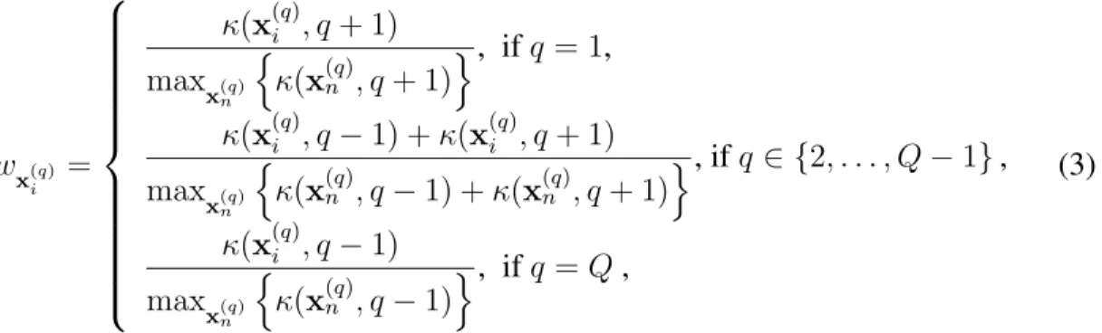
wx(q) i = κ(x(iq), q+ 1) maxx(q) n n κ(x(nq), q+ 1) o, ifq= 1, κ(x(iq), q−1) +κ(x(iq), q+ 1) maxx(q) n n κ(x(nq), q−1) +κ(x(nq), q+ 1) o, ifq∈ {2, . . . , Q−1}, κ(x(iq), q−1) maxx(q) n n κ(x(nq), q−1) o, ifq=Q, (3)
where the sum of the minimum distances of a pattern with respect to adjacent classes is normalized across all patterns of the class, so thatwx(q)
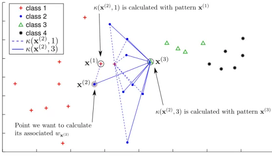
i has a maximum value of 1. Figure 1 shows the idea of minimum distances for each pattern with respect to the patterns of the adjacent classes. In this figure, patterns of the second class are consid-ered. The example illustrates how thewx(2) value is obtained for the patternx(2)marked
class 1 class 2 class 3 class 4
Figure 1: Illustration of the idea of minimum Pairwise Class Distances. All the mini-mum distances of patterns of classC2 regarding patterns of adjacent classes are painted
with lines.x(2) is the point we want to calculate its associatedwx(2).
with a circle. For distances betweenx(2)and class 1 patterns, the itemx(1)has the min-imum distance, soκ(x(2),1)is calculated by using this pattern. For distances between
x(2) and class 3 patterns,κ(x(2),3)is the minimum distance betweenx(2) andx(3).
By usingwx(q) i
, we can derive a latent variable value zi ∈ Z. Before continuing,
thresholds must be defined in order to stablish the intervals onZ which correspond to each class, so that calculated values for zi may be positioned on the proper interval.
Also, predicted valueszˆi of unseen data would be classified in different classes
accord-ing to these thresholds (see Subsection 3.3), in a similar way to any other threshold model. For the sake of simplicity,Z is defined between0and1, and the thresholds are
positioned in the uniform manner2 :
θ={θ1, θ2, . . . , θQ}={1/Q,2/Q, . . . ,1}. (4)
Consideringθ, the centrescq ∈ {c1, c2, . . . , cQ}forZ values belonging to classCq
are set to:c1 = 0,cQ = 1and
cq=
q Q −
1
2Q, q= 2,3, ...Q−1. (5) We now constructzivalues for training inputsx
(q)
i by considering the following criteria.
Ifx(iq)has similar minimum distancesκ(x(iq), q−1)andκ(x(iq), q+1)(and consequently a high value ofw
x(q)i ), the resultingzivalue should be closer toci, so that intuitively, we
consider this pattern aswell locatedwithin its class. Ifκ(x(iq), q−1)andκ(x(iq), q+ 1)
are very different (and consequently a low value ofwx(q) i
is obtained), the patternx(iq)is closer to one of these classes and so the correspondingzivalue should be closer to the
interval ofZvalues of the closest adjacent class,q−1orq+ 1. This idea is formailized in the following expression:
zi = φ x(iq) = c1+ (1−wx(1) i )· 1 Q, ifq= 1, cq−(1−wx(q) i )· 1 2Q, ifq∈ {2, . . . , Q−1}and κ(x(iq), q−1)≤κ(x(iq), q+ 1), cq+ (1−wx(q) i )· 1 2Q, ifq∈ {2, . . . , Q−1}and κ(x(iq), q−1)> κ(x(iq), q+ 1), cQ−(1−wx(Q) i )· 1 Q, ifq=Q, (6)
2This does not in any way hamper generality, as our regressors defininggwill be smooth non-linear
−4 −2 0 2 4 6 8 10 −4 −2 0 2 4 6 8 0.0000 0.0598 0.0007 0.0917 0.1166 0.1111 0.3925 0.3587 0.3504 0.3949 0.6820 0.6824 0.5536 1.0000 0.8798 0.9744 0.8812 class 1 class 2 class 3 class 4
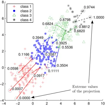
Figure 2: Example of the generatedzi values on a synthetic dataset with a linear order
relationship.
wherewx(q) i
is defined in Eq. (3),cqis the centre of class interval corresponding to Cq
(see Eq. (5)) and Q is the number of classes. Eq. (6) guarantees that all z values lie in the correct class interval3. This methodology for data projection is calledPairwise Class Distances(PCD).
3.2
Analysis of the proposed projection in synthetic datasets
For illustration purposes, we generated synthetic ordinal classification datasets inX ∈
R2 with four classes (Q = 4). Figure 2 shows the patterns of a synthetic dataset,
Syn-theticLinearOrder, with a linear order between classes, whereas Figure 3 shows Syn-theticNonLinearOrderdataset, with a non-linear ordinal relationship between classes.
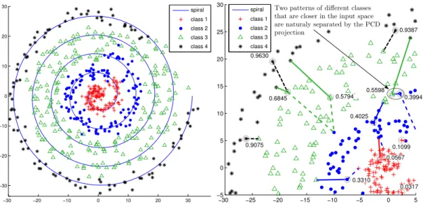
Points atSyntheticLinearOrderwere generated by adding an uniform noise to points of a line. Points inSyntheticNonLinearOrderwere generated by adding a Gaussian noise to points on a spiral. In both figures, points belonging to different classes are marked with different colours and symbols. Besides the points, the figures also illustrate ba-sic concepts of the proposed method on example points (surrounded by grey circles). For these points, the minimum distances are illustrated with lines of the corresponding class colour. The minimum distance of a point to the previous and next class patterns are marked with dashed and solid lines, respectively. For selected points we show the value of the PCD projection (calculated using Eq. (6)).
In Figure 2 it can be seen that thezvalue increases for patterns of the higher classes, and this value varies depending of the position of the patternx(q) in the space with re-spect to the patternsx(q−1)andx(q+1) of adjacent classes. Extreme values,z = 0.0and
z = 1.0correspond to the patterns more distant from the classes1andQrespectively (and with a maximumwx(q) value). SyntheticNonLinearOrder in Figure 3 is designed
to demonstrate that the PCD projection is suitable for more complex ordinal topologies of the data. This is, for any topology in a ordinal dataset, it is expected that patterns of classesq−1andq+ 1are always the closest ones to the patterns of classq, and PCD will take advantage from this situation to decide the relative order of the pattern within its class, even when this is produced in a non-linear manner.
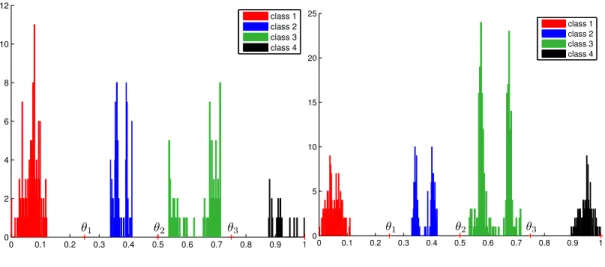
Figure 4a and Figure 4b show histograms of the PCD projections from the synthetic datasets in Figure 2 and Figure 3, respectively. The thresholdsθthat divide thezvalues of the different classes are also included. Observe that the z values of the different classes are clearly separated, and that they are compacted within a range which is always
−30 −20 −10 0 10 20 30 −30 −20 −10 0 10 20 30 class 1 class 2 class 3 class 4 spiral
(a) General disposition of the points of the dataset.
−30 −25 −20 −15 −10 −5 0 5 −5 0 5 10 15 20 25 30 0.0567 0.0317 0.1099 0.4025 0.3310 0.3994 0.5598 0.5794 0.6845 0.9387 0.9630 0.9075 class 1 class 2 class 3 class 4 spiral
(b) Upper left area of the dataset.
Figure 3: Example of the generatedzi values on the synthetic dataset with a non-linear
class order structure. Figure on the right shows a zooming over the upper left area at the center of the dataset shown on the left.
smaller than the range initially indicated by the thresholds. This is due to the scaling of thez values in Eq. (3), where thewx(q) value cannot be zero, so a pattern can never be
located ‘close’ to the boundary separating intervals of adjacent classes.
3.3
Algorithm for ordinal classification
Once the PCD projections have been obtained for all training inputs, we construct a new training set T0 =
n
(xi, φ(x
(yi)
i )|(xi,yi)∈T o
. Any generic regression tool can be trained on T0 to obtain the projection function g : X → Z. In this respect, our method is quite general, allowing the user to choose his or her favorite regression method or any other improved regression tool introduced in the future. The resulting algorithm, named Pairwise Class Distances for Ordinal Classification (PCDOC), is
de-0 0.1 0.2 0.3 0.4 0.5 0.6 0.7 0.8 0.9 1 0 2 4 6 8 10 12 class 1 class 2 class 3 class 4
(a)SyntheticLinearOrderdataset.
0 0.1 0.2 0.3 0.4 0.5 0.6 0.7 0.8 0.9 1 0 5 10 15 20 25 class 1 class 2 class 3 class 4 (b)SyntheticNonLinearOrderdataset.
Figure 4: Histograms of the PCD projection of the synthetic datasets.
scribed in two steps in Figure 5 and Figure 6.
It is expected that formulating the problem as a regression problem would help the model to capture the ordinal structure of the input and output spaces, and their relationship. In addition, due to the nature of the regression problem, it is expected that the performance of the classification task will be improved regarding metrics that consider the difference between the predicted and actual classes within the linear class order, such asM AE or AM AE, or the correlation between the target and predicted values, such asτb. Experimental results confirm this hypothesis in Section 4.3.
3.4
PCDOC performance analysis in some controlled experiments
Analysis of the influence of dimensionality and class overlapping. This section analyses the performance of the PCDOC algorithm under situations that may hamper classification: class overlapping and large dimensionality of the data. For this purpose, different synthetic datasets have been generated by sampling random points from Q
PCDOC Training: {g,θ}= PCDOCtr(T). Require: Training datasetT.
Ensure: Regressor (g) and thresholds (θ).
1: Calculate thresholdsθand centrescaccording to Eq. (4) and Eq. (5).
2: For each pattern, calculateziaccording to Eq. (6): zi =φ(x
(q)
i ).
3: Build a regressorg, consideringzas the regression response variable: z =g(x).
4: return {g,θ}
Figure 5: PCDOC regression training algorithm pseudocode. PCDOC Prediction: yˆ= PCDOCpr(x, g,θ).
Require: Regressor (g), thresholds (θ) and test input (x). Ensure: Predicted label (y).ˆ
1: Predict the latent variable value using the regressorg: zˆ=g(x).
2: Map the zˆvalue to the corresponding class using f as defined in Eq. (1): yˆ =
f(ˆz,θ).
3: return yˆ
Figure 6: PCDOC classification algorithm for unseen data.
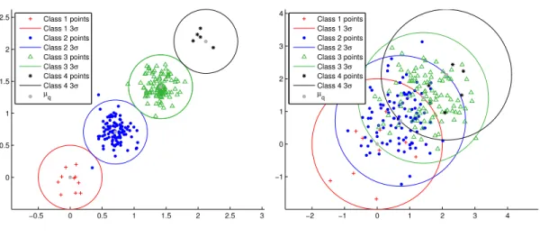
Gaussian distributions, whereQis the number of classes, so that each class points are random samples of the corresponding Gaussian distribution. In order to easily control the overlap of the classes, the variance (σ2) is kept constant independently of the number
of dimensions (K). In addition, the Qcentres (means µq) are set up in order to keep
the distance of1 between two adjacent class means independently of K. Under this situation, each coordinate of adjacent class means is separated by4µ = 1/
√
−0.5 0 0.5 1 1.5 2 2.5 3 0 0.5 1 1.5 2 2.5 Class 1 points Class 1 3σ Class 2 points Class 2 3σ Class 3 points Class 3 3σ Class 4 points Class 4 3σ µq
(a) Synthetic Gaussian dataset withσ= 0.167.
−2 −1 0 1 2 3 4 −1 0 1 2 3 4 Class 1 points Class 1 3σ Class 2 points Class 2 3σ Class 3 points Class 3 3σ Class 4 points Class 4 3σ µq
(b) Synthetic Gaussian dataset withσ= 0.667.
Figure 7: Synthetic Gaussian dataset example for two dimensions.
µ1 = 0,µ2 =µ1+4µ,µ3 =µ2+4µand so on.
The number of features tested (input space dimensionality) wereK ∈ {10,50,100}
and the different width values are σ ∈ {0.167,0.333,0.500,0.667,0.800,1.000}, so that 18 datasets were generated. The number of patterns for each class from one to four was 10, 100, 100 and 5. Figure 7 shows two of these datasets generated with different variance values forK = 2.
For these experiments, our approach uses the Support Vector Regression (SVR) algorithm as the model for the z variable (the method will be referred to as SVR-PCDOC). We have also included three methods as baseline methods: the C-Support Vector Classification (SVC) (Cortes and Vapnik, 1995; Vapnik, 1999), the Support Vec-tor Ordinal Regression with explicit constraints (SVOREX) (Chu and Keerthi, 2005, 2007) and the Kernel Discriminant Learning for Ordinal Regression (KDLOR) (Sun et al., 2010). As in the next experimental section (Section 4), the experimental design includes30stratified random splits (with 75%of patterns for training and the
remain-0.1 0.2 0.3 0.4 0.5 0.6 0.7 0.8 0.9 1 0.1 0.2 0.3 0.4 0.5 0.0 σ MAE SVC SVOREX KDLOR SVR−PCDOC (a)M AEwithK= 10. 0.1 0.2 0.3 0.4 0.5 0.6 0.7 0.8 0.9 1 0 0.1 0.2 0.3 0.4 0.5 0.6 0.7 0.8 0.9 1 σ AMAE SVC SVOREX KDLOR SVR−PCDOC (b)AM AEwithK= 10. 0.1 0.2 0.3 0.4 0.5 0.6 0.7 0.8 0.9 1 0.1 0.2 0.3 0.4 0.5 0.0 σ MAE SVC SVOREX KDLOR SVR−PCDOC (c)M AEwithK= 50. 0.1 0.2 0.3 0.4 0.5 0.6 0.7 0.8 0.9 1 0 0.1 0.2 0.3 0.4 0.5 0.6 0.7 0.8 0.9 1 σ AMAE SVC SVOREX KDLOR SVR−PCDOC (d)AM AEwithK= 50. 0.1 0.2 0.3 0.4 0.5 0.6 0.7 0.8 0.9 1 0.1 0.2 0.3 0.4 0.5 0.0 σ MAE SVC SVOREX KDLOR SVR−PCDOC (e)M AEwithK= 100. 0.1 0.2 0.3 0.4 0.5 0.6 0.7 0.8 0.9 1 0 0.1 0.2 0.3 0.4 0.5 0.6 0.7 0.8 0.9 1 σ AMAE SVC SVOREX KDLOR SVR−PCDOC (f)AM AEwithK= 100.
Figure 8:M AEandAM AEperformance for synthetic Gaussian dataset with distribu-tionx=N(µ, σ2I
ing for generalization). The meanM AE andAM AE generalization results are used for comparison purposes at Figure 8. For further details about experimental procedure, methods description and hyper-parameters optimization please refer to the next experi-mental section (Subsection 4.2).
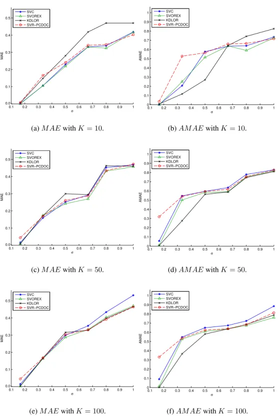
From the results depicted at Figure 8, we can generally conclude that the three methods, except KDLOR, have similar M AE performance degradation with the in-crease of class overlapping and dimensionality. Figure 8a shows that SVR-PCDOC have a slightly worse performance than SVC and SVOREX. However, in experiments with higherK (Figures 8c and 8e) the performance of the three ordinal methods varies in a similar way. In partigular, in Figure 8e we can observe that SVC performance decreases with high overlapping and high dimensionality, whereas the ordinal methods have similar performance here. From the analysis of the AM AE performance we can conclude that KDLOR outperforms the rest of the methods in cases of low class over-lapping. Regarding our method, we can conclude that compared with the other methods itsAM AEperformance is worse in the case of low class overlap. However, in general, our method seems more robust when the class overlap increases.
Analysis of the influence of data multimodality. This section extends the above experiments to the case of multimodal data, the datasets are generated with K = 2
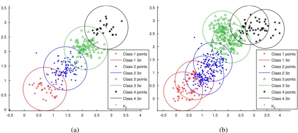
and σ2 = 0.25, and the number of modes per class is varied. Figure 9a presents the unimodal case. The datasets with more modes per class are generated in the following way. A Gaussian distribution is set up as in the previous section, with center µq. For
-0.5 0 0.5 1 1.5 2 2.5 3 3.5 4 0 0.5 1 1.5 2 2.5 3 3.5 Class 1 points Class 1 3σ Class 2 points Class 2 3σ Class 3 points Class 3 3σ Class 4 points Class 4 3σ µq (a) -0.5 0 0.5 1 1.5 2 2.5 3 3.5 4 0 0.5 1 1.5 2 2.5 3 3.5 Class 1 points Class 1 3σ Class 2 points Class 2 3σ Class 3 points Class 3 3σ Class 4 points Class 4 3σ µq (b)
Figure 9: Illustration of the unimodal and bimodal cases of the synthetic Gaussian dataset example forK = 2andσ2 = 0.25.
1 2 3 4 0 0.02 0.04 0.06 0.08 0.1 0.12 0.14 modes MAE SVC SVOREX KDLOR SVR−PCDOC (a)M AEperformance. 1 2 3 4 0 0.05 0.1 0.15 0.2 0.25 modes AMAE SVC SVOREX KDLOR SVR−PCDOC (b)AM AEperformance.
Figure 10: M AE andAM AE performance for synthetic Gaussian dataset with distri-butionx=N(µ, σ2I
K×K)andx∈X⊆RK, whereIK×Kis the identity matrix (being
K = 2andσ2 = 0.25for all the synthetic datasets).
the hyper-sphere with centerµq and radius0.75. Then, patterns are sampled from each
distribution. For each class, we considered different number of modes, from one mode to four modes. The number of patterns generated for each mode was 36, 90, 90 and 24
for class 1, 2, 3 and 4, respectively, using the same number for all modes of a class. An example of the bimodal case (two Gaussian distributions per class) is shown in Figure 9b, having 72, 180, 180 and 48 patterns for class 1, 2, 3 and 4, respectively.
Experiments were carried out as in the previous section, and M AE and AM AE generalization results are depicted in Figure 10. RegardingM AE, Figure 10a reveals that the fours methods perform similarly in datasets with one and four modes but they differ on performance for the two and three modes. Only considering M AE, SVR-PCDOC has the worse performance in case two and three. Nevertheless, considering AM AE results at Figure 10b, SVRPCDOC and KDLOR achieve the best results. The different behaviour of the methods depending on the performance measure can be ex-plained by observing the nature of the bimodal dataset (see Figure 9b), where the ma-jority of the patterns are from classes two and three. In this context, the optimization done by SVOREX and SVC can move the decision thressholds to better classify pat-terns of these two classes at the expense of misclassifying class one and four patpat-terns, especially patterns of those classes placed on the class boundaries (see Figure 9b).
4
Experiments
In this section we report on extensive experiments that were performed to check the competitiveness of the proposed methodology. Source code of the proposed method, synthetic datasets analysis code and real ordinal data sets partitions used for the exper-iments are available at a public website4.
4.1
Ordinal classification datasets and experimental design
To the best of our knowledge, there are no public specific datasets repositories for real ordinal classification problems. The ordinal regression benchmark datasets repository provided by Chu et. al (Chu and Ghahramani, 2005) is the most widely used repository in the literature. However, these datasets are not real ordinal classification datasets but regression ones. To turn regression into ordinal classification, the target variable was discretized intoQ different bins (representing classes), with equal frequency or equal width. However, there are potential problems with this approach. If equal frequency la-belling is considered, the datasets do not exhibit some characteristics of typical complex classification tasks, such as class imbalance. On the other hand, severe class imbalance can be introduced by using the same binning width. Finally, as the actual target regres-sion variable exists with observed values, the classification problem can be simpler than on those datasets where the variablezis really unobservable and has to be modelled.
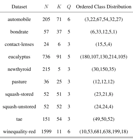
We have therefore decided to use a set of real ordinal classification datasets pub-licly available at the UCI (Asuncion and Newman, 2007) and mldata.orgrepositories (Sonnenburg, 2011) (see Table 1 for data description). All of them are ordinal classi-fication problems, although one can find literature where the ordering information is discarded. The nature of the target variable is now analysed for two example datasets.
bondratedataset is a classification problem where the purpose is to assign the right or-dered category to bonds, being the category labels{C1 = AAA, C2 = AA, C3 = A,
C4 = BBB, C5 = BB}. These labels represent the quality of a bond and are assigned
by credit rating agencies, AAA being the highest quality and BB the worst one. In this case, classesAAA, AA,Aare more similar than classes BBBandBBso that no
assumptions should be done about the distance between classes both in the input and latent space. Other example iseucalyptusdataset, in this case the problem is to predict which eucalyptus seedlots are best for soil conservation in a seasonally dry hill country. Being the classes{C1 = none, C2 = low, C3 = average, C4 = good, C5 = best}, it
cannot be assumed an equal width for each class in the latent space.
Regarding the experimental set up, 30different random splits of the datasets have been considered, with75%and25%of the instances in the training and test sets respec-tively. The partitions were the same for all compared methods, and, since all of them are deterministic, one model was obtained and evaluated (in the test (generalization) set), for each split. All nominal attributes were transformed into as many binary attributes as the number of categories. All the datasets were property standardized.
4.2
Existing methods used for comparison purposes
For comparison purposes, different state-of-the-art methods have been included in the experimentation (all of them mentioned in the Introduction):
• Gaussian Processes for Ordinal Regression (GPOR) (Chu and Ghahramani, 2005), presents a probabilistic kernel approach to ordinal regression based on Gaussian processes where a threshold model that generalizes theprobit function is used as the likelihood function for ordinal variables. In addition, Chu applies the automatic relevance determination (ARD) method proposed by (Mackay, 1994) and (Neal, 1996) to the GPOR model. When using GPOR with ARD feature se-lection, we will refer the algorithm to as GPOR-ARD.
Table 1: Datasets used for the experiments (N is the number of patterns, K is the number of attributes andQis the number of classes).
Dataset N K Q Ordered Class Distribution automobile 205 71 6 (3,22,67,54,32,27) bondrate 57 37 5 (6,33,12,5,1) contact-lenses 24 6 3 (15,5,4) eucalyptus 736 91 5 (180,107,130,214,105) newthyroid 215 5 3 (30,150,35) pasture 36 25 3 (12,12,12) squash-stored 52 51 3 (23,21,8) squash-unstored 52 52 3 (24,24,4) tae 151 54 3 (49,50,52) winequality-red 1599 11 6 (10,53,681,638,199,18)
Keerthi, 2007), proposes two new support vector approaches for ordinal regres-sion. Here, multiple thresholds are optimized in order to define parallel discrim-inant hyperplanes for the ordinal scales. The first approach, with explicit in-equality constraints on the thresholds, derive the optimal conditions for the dual problem, and adapt the SMO algorithm for the solution, and we will refer to it as SVOREX. In the second approach, the samples in all the categories are allowed to contribute errors for each threshold, therefore there is no need of including the inequality constraints in the problem. This approach is named a SVOR with implicit constraints (SVORIM).
• RED-SVM(Li and Lin, 2007) applies the reduction from cost-sensitive ordinal ranking to weighted binary classification (RED) framework to SVM. The RED method can be summarized in the following three steps. First, transform all train-ing samples into extended samples by ustrain-ing a codtrain-ing matrix, and weighttrain-ing these samples with a cost matrix. Second, all the extended examples are jointly learned by a binary classifier with confidence outputs, aiming at a low weighted0/1loss. Last step is used to convert the binary outputs to a rank. In this paper, the coding matrix considered is the identity and the cost matrix is the absolute value matrix, applied to the standard binary soft-margin SVM.
• A Simple Approach to Ordinal Regression (ASAOR) by Frank et. al (Frank and Hall, 2001) is a general method that enables standard classification algorithms to make the use of order information in attributes. For the training process, the method transforms theQ-class ordinal problem intoQ−1binary class problems. Any ordinal attribute with ordered values is converted intoQ−1binary attributes. The prediction of new instances class is done by estimating the probability of belonging to each of the Qclasses with theQ−1models. In the current work, the C4.5 method available in Weka (Hall et al., 2009) is used as the underlying classification algorithm since this is the one initially employed by the authors of ASAOR. In this way, the algorithm is identified as ASAOR(C4.5).
• The Proportional Odds Model (POM) is one of the first models specifically designed for ordinal regression (McCullagh, 1980). The model is based on the assumption of stochastic ordering of the spaceX. Stochastic ordering is satisfied
by a monotonic function (the model) that defines a probability density function over the class labels for a given feature vectorx. Due to the thresholds that divide the monotonic function values corresponding to different classes, this method was the first one to be named a threshold model. The main problem associated with this model is that the projection is done by considering a linear combination of the inputs (linear projection), which hinders its performance. For the POM model, themnrfitfunction of Matlab software has been used.
• Kernel Discriminant Learning for Ordinal Regression (KDLOR)(Sun et al., 2010) extends the Kernel Discriminant Analysis (KDA) using a rank constraint. The method looks for the optimal projection that maximizes the separation be-tween the projection of the different classes and minimizes the intra-class dis-tance as in traditional discriminant analysis for nominal classes. Crucially, how-ever, the order of the classes in the resulting projection is also considered. The authors claim that, compared with the SVM based methods, the KDA approach takes advantage of the global information of the data and the distribution of the classes, and also reduces the computational complexity of the problem.
• Support Vector Machine (SVM)(Cortes and Vapnik, 1995; Vapnik, 1999) nom-inal classifier is included in the experiments in order to establish a baseline nomi-nal performance. C-Support Vector Classification (SVC) available in libSVM 3.0 (Chang and Lin, 2011) is used as the SVM classifier implementation. In order to deal with the multiclass case, a “1-versus-1” approach has been considered, following the recommendations of Hsu and Lin (Hsu and Lin, 2002).
In our approach, the Support Vector Regression (SVR) algorithm is used as the model for thezvariable. The method will be referred to by the acronym SVR-PCDOC. The-SVR available in libSVM is used. The authors of GPOR, SVOREX, SVORIM and RED-SVM provide publicly available software implementations of their methods5. In the case of KDLOR, this method has been implemented by the authors using Matlab software (Perez-Ortiz et al., 2011).
Model selection is an important issue and involves selecting the best hyper-parameter combination for all the methods compared. All the methods were configured to use the Gaussian kernel. For the support vector algorithms, i.e. SVC, RED-SVM, SVOREX, SVORIM and -SVR, the corresponding hyper-parameters (regularization parameter, C, and width of the Gaussian functions,γ), were adjusted using a grid search over each
of the30training sets by a 5-fold nested cross-validation with the following ranges: C∈ {103,102, . . . ,10−3}and γ ∈ {103,102, . . . ,10−3}. Regarding -SVR, the additional
parameter has to be adjusted. The range considered was ∈ {103,102,101,100}. For KDLOR, the width of the Gaussian kernel was adjusted by using the rangeγ ∈ {103,102, . . . ,10−3}, and the regularization parameter, u, for avoiding the singularity
problem values wereu ∈ {10−2,10−3, . . . ,10−5}. POM and ASAOR(C4.5) methods have not hyper-parameters. Finally, GPOR-ARD has no hyper-parameters to fix, since the method optimizes the associated parameters itself.
5GPOR (http://www.gatsby.ucl.ac.uk/˜chuwei/ordinalregression.html),
SVOREX and SVORIM (http://www.gatsby.ucl.ac.uk/˜chuwei/svor.htm) and
For all the methods, theM AEmeasure is used as the performance metric for guid-ing the grid search to be consistent with the authors of the different state-of-the-art methods. The grid search procedure of SVC at libSVM has been modified in order to useM AEas the criteria for hyper-parameters selection.
4.3
Performance results
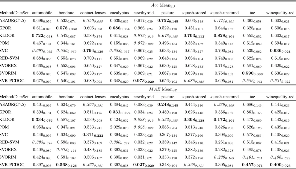
Tables 2 and 3 outline the results through the mean and standard deviation (SD) of AccG, M AEG,AM AEGandτbGacross the30hold-out splits, where the subindexG
indicates that results were obtained on the (hold-out) generalization fold. As a summary, Table 4 shows, for each performance metric, the mean values of the metrics across all the datasets, and the mean ranking values when comparing the different methods (R = 1 for the best performing method and R = 9 for the worst one). To enhance readability, in Tables 2, 3 and 4 the best and second-best results are in bold face and italics, respectively.
Table 2: Comparison of the proposed method to other ordinal classification methods and SVC. The mean and standard deviation (SD) of the generalization results are reported for each dataset. The best statistical result is in bold face and the second best result in italics.
AccMeanSD
Method/DataSet automobile bondrate contact-lenses eucalyptus newthyroid pasture squash-stored squash-unstored tae winequality-red ASAOR(C4.5) 0.6960.059 0.5330.074 0.7500.085 0.6390.036 0.9170.039 0.7520.145 0.6030.118 0.7740.101 0.3950.058 0.6030.021 GPOR 0.6110.073 0.5780.032 0.6060.093 0.6860.034 0.9660.024 0.5220.178 0.4510.101 0.6440.162 0.3280.041 0.6060.015 KLDOR 0.7220.058 0.5420.087 0.5890.174 0.6110.028 0.9720.019 0.6780.125 0.7030.112 0.8280.104 0.5550.052 0.6030.017 POM 0.4670.194 0.3440.161 0.6220.138 0.1590.036 0.9720.022 0.4960.154 0.3820.152 0.3490.143 0.5120.089 0.5940.017 SVC 0.6970.062 0.5560.069 0.7940.129 0.6530.037 0.9670.025 0.6330.134 0.6560.127 0.7000.082 0.5390.062 0.6360.021 RED-SVM 0.6840.055 0.5530.073 0.7000.111 0.6510.024 0.9690.022 0.6480.134 0.6640.104 0.7490.086 0.5220.074 0.6180.022 SVOREX 0.6650.068 0.5530.096 0.6500.127 0.6470.029 0.9670.022 0.6300.125 0.6280.133 0.7180.128 0.5810.060 0.6290.022 SVORIM 0.6390.076 0.5470.092 0.6330.127 0.6390.028 0.9690.021 0.6670.120 0.6390.118 0.7640.103 0.5900.066 0.6300.022 SVR-PCDOC 0.6780.060 0.5400.101 0.6890.095 0.6480.029 0.9730.020 0.6560.103 0.6850.123 0.6950.084 0.5820.064 0.6310.022 M AEMeanSD
Method/DataSet automobile bondrate contact-lenses eucalyptus newthyroid pasture squash-stored squash-unstored tae winequality-red ASAOR(C4.5) 0.4010.095 0.6240.079 0.3670.154 0.3840.042 0.0830.039 0.2480.145 0.4440.140 0.2390.109 0.6860.146 0.4410.023 GPOR 0.5940.131 0.6240.062 0.5110.175 0.3310.038 0.0340.024 0.4890.190 0.6260.148 0.3560.162 0.8610.155 0.4250.017 KLDOR 0.3340.076 0.5870.107 0.5390.208 0.4240.032 0.0280.019 0.3220.125 0.3080.128 0.1720.104 0.4730.069 0.4430.019 POM 0.9530.687 0.9470.321 0.5330.241 2.0290.070 0.0280.022 0.5850.204 0.8130.248 0.8260.230 0.6260.126 0.4390.019 SVC 0.4460.095 0.6240.090 0.3110.222 0.3940.042 0.0330.025 0.3670.134 0.3770.160 0.3080.090 0.5780.083 0.4080.020 RED-SVM 0.3930.073 0.5980.088 0.3780.169 0.3800.027 0.0320.022 0.3590.142 0.3460.110 0.2510.086 0.5150.087 0.4190.021 SVOREX 0.4080.089 0.5730.121 0.4890.185 0.3920.031 0.0330.022 0.3700.125 0.3820.139 0.2820.128 0.4850.078 0.4080.023 SVORIM 0.4240.090 0.5910.102 0.5060.167 0.3950.035 0.0310.021 0.3330.120 0.3720.126 0.2390.109 0.4610.081 0.4060.022 SVR-PCDOC 0.3970.093 0.5680.126 0.3670.154 0.3920.038 0.0270.020 0.3480.104 0.3260.141 0.3050.084 0.4570.071 0.4000.023 34
Table 3: Comparison of the proposed method to other ordinal classification methods and SVC. The mean and standard deviation (SD) of the generalization results are reported for each dataset. The best statistical result is in bold face and the second best result in italics.
AM AEMeanSD
Method/DataSet automobile bondrate contact-lenses eucalyptus newthyroid pasture squash-stored squash-unstored tae winequality-red
ASAOR(C4.5) 0.5110.104 1.2260.175 0.3150.124 0.4280.045 0.1150.056 0.2480.145 0.5020.192 0.2560.149 0.6890.151 1.0450.080 GPOR 0.7920.200 1.3600.122 0.6510.286 0.3620.040 0.0620.049 0.4890.190 0.7970.234 0.4430.226 0.8630.164 1.0650.065 KLDOR 0.3450.104 1.0370.270 0.5190.280 0.4260.038 0.0590.040 0.3220.125 0.3490.156 0.3090.180 0.4710.070 1.2580.069 POM 1.0260.800 1.1030.403 0.5350.275 1.9900.048 0.0500.040 0.5850.204 0.8150.251 0.7910.332 0.6270.128 1.0850.037 SVC 0.4860.125 1.2650.183 0.3070.277 0.4330.048 0.0600.051 0.3670.134 0.4460.189 0.4440.163 0.5760.083 1.1190.069 RED-SVM 0.4680.096 1.1840.225 0.3850.198 0.4140.030 0.0570.049 0.3590.142 0.3910.149 0.3480.159 0.5130.086 1.0680.069 SVOREX 0.5180.096 1.0720.217 0.5170.303 0.4110.034 0.0540.042 0.3700.125 0.4330.172 0.4260.157 0.4840.079 1.0950.067 SVORIM 0.5230.105 1.1140.233 0.5890.259 0.4200.043 0.0550.042 0.3330.120 0.4270.148 0.3670.140 0.4590.081 1.0930.072 SVR-PCDOC 0.4400.128 0.9690.224 0.4200.098 0.4000.043 0.0450.040 0.3480.104 0.3600.184 0.3960.158 0.4550.071 1.0400.096 τb MeanSD
Method/DataSet automobile bondrate contact-lenses eucalyptus newthyroid pasture squash-stored squash-unstored tae winequality-red
ASAOR(C4.5) 0.7410.069 0.1430.159 0.6040.216 0.8020.025 0.8530.067 0.7780.132 0.4150.245 0.6920.145 0.2430.177 0.4960.036 GPOR 0.5570.118 0.0000.000 0.3480.304 0.8300.020 0.9380.045 0.4610.314 0.0750.211 0.4200.331 −0.0180.108 0.5230.026 KLDOR 0.7930.056 0.3560.257 0.4480.273 0.7860.017 0.9480.034 0.7180.133 0.6460.160 0.7640.161 0.4770.114 0.4600.028 POM 0.4950.283 0.2900.302 0.4580.309 0.0080.038 0.9490.040 0.4630.237 0.1690.304 0.1090.305 0.3170.129 0.4970.025 SVC 0.6950.077 0.1210.177 0.6010.300 0.7830.025 0.9390.045 0.6980.133 0.5410.240 0.5990.140 0.3750.110 0.5160.027 RED-SVM 0.7510.054 0.2540.247 0.5770.242 0.8000.017 0.9430.041 0.7070.129 0.6010.148 0.6620.108 0.4170.120 0.5250.030 SVOREX 0.7490.062 0.3690.216 0.4250.304 0.7940.019 0.9410.040 0.6910.115 0.5340.207 0.5920.212 0.4450.110 0.5310.028 SVORIM 0.7480.065 0.2990.230 0.3820.269 0.7920.020 0.9440.038 0.7100.114 0.5420.167 0.6560.187 0.4820.118 0.5330.030 SVR-PCDOC 0.7440.076 0.4550.218 0.6200.217 0.7950.024 0.9520.037 0.7120.102 0.6100.201 0.6020.133 0.4930.101 0.5420.033 35
Regarding Tables 2 and 3, it can be seen that the majority of methods are very com-petitive. The best performing method depends on the considered performance metric, as it can be seen from the mean rankings. This is also true when separately consid-ering each of the datasets, and the performance for some datasets varies noticeably if AM AEG is considered instead of M AEG (see bondrate, contact-lenses,
eucalyp-tus, squash-unstored andwinequality-red). In the case of winequality-red, it happens that the second worse method in M AEG, ASAOR(C4.5), is the second best one for
AM AEG. It is worthwhile to mention that for pasture dataset the mean M AEG and
AM AEG are the same, which is due to the fact that pasture is a perfectly balanced
dataset (see Section 2.2). In the case oftae, M AEG and AM AEG are very similar
since the patterns distribution across classes is very similar. RegardingτbG, it is
in-teresting to highlight that a value close to zero of this metric reveals that the classifier predictions are not related to the real values, this is, the classifier performance is sim-ilar to the performance of a trivial classifier. This happens for GPOR method in the
bondrate,squash-storedandtaedatasets, and for POM in theeucalyptusdataset. From Table 4, it can be observed how best mean value across the different datasets is not always translated into best mean ranking (seeAccGandRAccG columns). We now
analyze the results in greater detail, highlighting the best and second best performances. When consideringAccG, SVC is clearly the best method, both in average performance
and ranking. KDLOR and SVR-PCDOC are the second best methods, in average value and ranking, respectively. However, results are very different for all the other measures, where the order is included in the evaluation. The best method in averageM AEG and
Table 4: Mean results of accuracy (AccG), M AE (M AEG), AM AE (AM AEG) and
τb (τbG) and mean ranking (RAccG, RM AEG, RAM AEG andRτbG) for the generalization
sets.
Method/Metric AccG RAccG M AEG RM AEG AM AEG RAM AEG τbG RτbG
GPOR 0.666 5.40 0.392 5.25 0.534 4.90 0.577 5.20 ASAOR(C4.5) 0.600 6.50 0.485 7.00 0.688 7.00 0.413 7.50 KDLOR 0.680 4.20 0.363 4.00 0.509 3.80 0.640 3.60 POM 0.490 7.90 0.778 7.80 0.861 7.00 0.375 6.90 SVC 0.683 3.60 0.385 5.55 0.550 6.20 0.587 6.20 RED-SVM 0.676 4.15 0.367 4.00 0.519 4.10 0.624 4.00 SVOREX 0.667 5.05 0.382 4.75 0.538 4.90 0.607 5.00 SVORIM 0.672 4.40 0.376 4.05 0.538 4.80 0.609 4.20 SVR-PCDOC 0.678 3.80 0.359 2.60 0.487 2.30 0.653 2.40
RED-SVM, having similar meanM AEG. AM AE is a better alternative than M AE
when the distribution of patterns is not balanced, and this is clearly the case for several datasets (see Table 1). The best values for meanAM AEG and mean ranking are
ob-tained by SVR-PCDOC, and the second ones are those reported by KDLOR. Finally, theτbG is revealing the most clear differences. When using this metric, the best mean
values and ranks are reported by SVR-PCDOC, followed by KDLOR.
4.4
Statistical comparisons between methods
To quantify whether a statistical difference exists between any of these algorithms, a procedure for comparing multiple classifiers over multiple datasets is employed (Demˇsar, 2006). First of all, a Friedman’s non-parametric test (Friedman, 1940) with a
signifi-cance level ofα = 0.05has been carried out to determine the statistical significance of the differences in the mean ranks of Table 4 for each different measure. The test rejected the null-hypothesis stating that the differences in mean rankings of AccG, M AEG,
AM AEG and τbG obtained by the different algorithms were statistically significant
(withα = 0.05). Specifically, the confidence interval for this number of datasets and algorithms is C0 = (0,F(α=0.05) = 2.070), and the corresponding F-value for each
metric were3.257∈/ C0,4.821 ∈/ C0,4.184∈/ C0and5.099 ∈/ C0, respectively.
On the basis of this rejection, the Nemenyi post-hoc test is used to compare all clas-sifiers to each other (Demˇsar, 2006). This test considers that the performance of any two classifiers is deemed significantly different if their mean ranks differ by at least the critical difference (CD), which depends on the number of datasets and methods. A5%
significance confidence was considered (α= 0.05) to obtain this CD and the results can be observed in Figure 11, which shows CD diagrams as proposed in (Demˇsar, 2006). Each method is represented as a point in a raking scale, corresponding to its mean rank-ing performance. CD segments are included to measure the separation needed between methods in order to assess statistical differences. Red lines group algorithms were sta-tistically different mean ranking performance cannot be assessed. Table 4 should also be considered when interpreting this graph.
Figure 11a shows that SVC, i.e. the nominal classifier, has the best performance in Acc, this is, when not considering the order of the label prediction errors, and
SVR-PCDOC has the second best one. RED-SVM, KDLOR and SVORIM have similar performance here. In Figure 11b, the best mean ranking is for SVR-PCDOC, and SVORIM, KDLOR and RED-SVM have similar performance. However, when
con-8 7 6 5 4 3 SVC SVR-PCDOC RED-SVM KDLOR POM GPOR ASAOR(C4.5) SVOREX SVORIM
(a) Nemenyi CD diagram comparing generalizationAccmean rankings of the different methods.
8 7 6 5 4 3 2 CD SVR-PCDOC RED-SVM KDLOR SVORIM POM GPOR SVC ASAOR(C4.5) SVOREX
(b) Nemenyi CD diagram comparing the generalization M AE mean rankings of the different methods.
7 6 5 4 3 2 CD SVR-PCDOC KDLOR RED-SVM SVORIM GPOR POM SVC SVOREX ASAOR(C4.5)
(c) Nemenyi CD diagram comparing the generalizationAM AE mean rankings of the different methods.
8 7 6 5 4 3 2 CD SVR-PCDOC KDLOR RED-SVM SVORIM GPOR POM SVC ASAOR(C4.5) SVOREX
(d) Nemenyi CD diagram comparing the generalizationτbmean rankings of the different methods.
Figure 11: Ranking test diagrams for the mean generalizationAcc,M AE,AM AE and τb.
Table 5: Differences and Critical Difference (CD) value in rankings in the Bonferroni-Dunn test, using SVR-PCDOC as the control method.
Method
Metric ASAOR(C4.5) GPOR KDLOR POM SVC RED-SVM SVOREX SVORIM
Acc 1.60 2.70 0.40 4.10• 0.20 0.35 1.25 0.60
M AE 2.65 4.40• 1.40 5.20• 2.95 1.40 2.15 1.45
AM AE 2.60 4.70• 1.50 4.70• 3.90• 1.80 2.60 2.50
τb 2.80 5.10• 1.20 4.50• 3.80• 1.60 2.60 1.80 Bonferroni-Dunn Test:CD(α=0.05)= 3.336
•: Statistical difference withα= 0.05
sideringAM AE, it can be seen at Figure 11c that SVR-PCDOC mean ranking distance to the other methods increases, specifically for RED-SVM and SVORIM. Finally, Fig-ure 11d shows the mean rank CD diagram forτbwhere SVR-PCDOC is still having the
best mean performance.
It has been noticed that the Nemenyi approach comparing all classifiers to each other in a post-hoc test is not as sensitive as the approach comparing all classifiers to a given classifier (a control method) (Demˇsar, 2006). The Bonferroni-Dunn test allows this latter type of comparison and, in our case, it is done using the proposed method as the control method for the four metrics. The results of the Bonferroni-Dunn test forα = 0.05can be seen in Table 5, where the corresponding critical values are included. From the results of this test, it can be concluded than SVR-PCDOC does not report a statistically significant difference with respect to the SVM ordinal regression methods, KDLOR and ASAOR(C4.5), but it does when it is compared to POM for all the metrics and compared to GPOR for the ordinal metrics. Moreover, there are
significant differences with respect to SVC, when consideringAM AE andτb.
From the above experiments, we can conclude that the reference (baseline) nom-inal classifier, SVC, is improved with statistical differences when considering ordnom-inal classification measures. Regarding ASAOR(C4.5), SVOREX, SVORIM, KDLOR and RED-SVM, whereas the general performance is slightly better, there are no statistically significant differences favouring any of the methods.
As a summary of the experiments, two important conclusions can be drawn about the performance measures: When imbalanced datasets are considered,AccG is clearly
omitting important aspects of ordinal classification and so does M AEG. If the
com-parative performance is taken into account, KDLOR and SVR-PCDOC appear to be very good classifiers when the objective is to improveAM AEGandτG. The best mean
ranking performance is obtained by our method proposed in this paper.
4.5
Latent space representations of the ordinal classes
In the previous section we have shown that our simple and intuitive methodology can compete on equal footing with established more complex and/or less direct methods for ordinal classification. In this section we complement this performance based compar-ison with a deeper analysis of the main ingredient of our and other related approaches to ordinal classification - projection onto the one-dimesional (latent) space naturally representing the ordinal nature of the class organization. In particular, we study how non-linear latent variable models, SVR-PCDOC, KDLOR, SVOREX and SVORIM or-ganize their one-dimensional latent space data projections. For comparison purposes, the latent variable Z values of the training and generalization data of the first fold of
0.1 0.2 0.3 0.4 0.5 0.6 0.7 0.8 0.9 1 0 0.2 0.4 relative frequen cy freq. thres q
(a) SVR-PCDOC train PCD histogram.
0.1 0.2 0.3 0.4 0.5 0.6 0.7 0.8 0.9 1 0 0.2 0.4 relative frequen cy freq. thres q
(b) SVR-PCDOC trainZˆhistogram.
0.1 0.2 0.3 0.4 0.5 0.6 0.7 0.8 0.9 1 0 0.2 0.4 relative frequen cy freq. thres q
(c) SVR-PCDOC generalization PCD histogram.
0.1 0.2 0.3 0.4 0.5 0.6 0.7 0.8 0.9 1 0 0.2 0.4 relative frequen cy freq. thres q
(d) SVR-PCDOC generalizationZˆhistogram.
0.1 0.2 0.3 0.4 0.5 0.6 0.7 0.8 0.9 1
Class 1 Class 2 Class 3 thres q
(e) SVR-PCDOC trainZˆprediction.
Class 1 Class 2 Class 3 thres q
0.1 0.2 0.3 0.4 0.5 0.6 0.7 0.8 0.9 1
(f) SVR-PCDOC generalizationZˆprediction.
Figure 12: PCD projection and SVR-PCDOC’s histograms and Zˆ prediction corre-sponding to the latent variable of the tae dataset: train PCD, train predicted Zˆ by SVR-PCDOC, generalization PCD and generalization predicted Zˆ by SVR-PCDOC. Generalization results areAcc= 0.582,M AE = 0.457,AM AE = 0.455,τb = 0.493.
taedataset are shown (Figure 12). Both histograms and values are plotted so that the behaviour of the models can be analysed. In the case of PCDOC, the PCD projection is also included to see whether the regressor model is close to the PCDOC projection. The histograms represent relative frequency of the projections. SVORIM histograms and latent variable values are not presented since they are similar to the SVOREX ones in the selected dataset.
We first analyse the SVR-PCDOC method. From PCD projections in Figure 12a we deduce that classesC1 andC2 contain patterns that are very close in the input space –
projection of some patterns fromC2 lies near the threshold that divides theZvalues for
the two classes. Analogous comment applies to classesC2andC3. The regressor seems
to have learnt the imposed projection reasonably well since the predicted latent values have a histogram similar to the training PCD projection histogram. The generalization PCD projections (Figure 12c) have similar characteristics as the training ones6. Note the concentration of values aroundzˆ = 0.5on the prediction of the generalization Z. This concentration of values is due to wrong prediction of class C1 and C3 patterns
that were both assigned toC2. This behaviour can be better seen in Figures 12e and
12f, where the modelled latent value for each pattern is shown together with its class label. Indeed, during training someC1 andC2 patterns were mapped to positions near
the thresholds. This is probably caused by noise or overlapping class distribution in the input space.
Figure 13 presents latent variable values of KDLOR. The KDLOR method projects 6There are much less patterns in the hold-out set than in the training set, making direct comparison of
the data onto the latent space by minimizing the intra-class distance while maximizing the inter-class distance of the projections. As a result, the latent representations of the data are quite compact for each class (see training projection histogram in Figure 13a). While this philosophy often leads to superior classification results, the projections are not reflecting the structure of patterns within a single class, that is, the ordinal nature of the data is not fully captured by the model. In addition, KDLOR projections occur in the wrong bins more often than in the case of SVR-PCDOC (see generalization projections
Zin Figure 13d)).
Finally, Figure 14 presents latent representations of patterns by the SVOREX model. As in the KDLOR case, (except for a few patterns) the training latent representations are highly compact within each class. Again, the relative structure of patterns within their classes is lost in the projections.
In both models, KDLOR and SVOREX, there is a pressure in the model construc-tion phase to find 1-dimensional projecconstruc-tions of the data that result in compact classes, while maximizing the inter-class separation. In the case of KDLOR this is explicitly formulated in the objective function. On the other hand, the key idea behind SVM based approaches is margin maximization. Data projections that maximize inter-class margins implicitly make the projected classes compact. We hypothesise that the pres-sure for compact within-class latent projections can lead to poorer generalization per-formance, as illustrated in Figure 14d. In the case of overlapping classes the drive for compact class projections can result in locally highly non-linear projections of the overlapping regions, over which we do not have a direct control (unlike in the case of PCDOC, where the non-linear projection is guided by the relative positions of points
−0.015 −0.01 −0.005 0 0.005 0.01 0 0.2 0.4 relative frequen cy freq. thres q
(a) KDLOR trainZˆhistogram.
−0.015 −0.01 −0.005 0 0.005 0.01 0 0.2 0.4 relative frequen cy freq. thres q
(b) KDLOR generalizationZˆhistogram.
−0.015 −0.01 −0.005 0 0.005 0.01
Class 1 Class 2 Class 3 thres q
(c) KDLOR trainZˆprediction.
−0.015 −0.01 −0.005 0 0.005 0.01
Class 1 Class 2 Class 3 thres q
(d) KDLOR generalizationZˆprediction.
Figure 13: Prediction of train and generalizationZˆvalues corresponding to KDLOR at
taedataset. Generalization results areAcc = 0.555, M AE = 0.473,AM AE = 0.471, τb = 0.477.
with respect to the other classes). Having such highly expanding projections can result in test points being projected to wrong classes in an arbitrary manner. Even though we provide detailed analysis for one dataset and one fold only, the observed tendencies were quite general across the data sets and hold-out folds.