Towards Optimized Fine-Grained Pricing of
IaaS Cloud Platform
Hai Jin,
Senior Member, IEEE,
Xinhou Wang, Song Wu,
Member, IEEE,
Sheng Di,
Member, IEEE,
Xuanhua Shi,
Member, IEEE
Abstract—Although many pricing schemes in IaaS platform are already proposed with pay-as-you-go and subscription/spot market policy to guarantee service level agreement, it is still inevitable to suffer from wasteful payment because of coarse-grained pricing scheme. In this paper, we investigate an optimized fine-coarse-grained and fair pricing scheme. Two tough issues are addressed: (1) the profits of resource providers and customers often contradict mutually; (2) VM-maintenance overhead like startup cost is often too huge to be neglected. Not only can we derive an optimal price in the acceptable price range that satisfies both customers and providers simultaneously, but we also find a best-fit billing cycle to maximize social welfare (i.e., the sum of the cost reductions for all customers and the revenue gained by the provider). We carefully evaluate the proposed optimized fine-grained pricing scheme with two large-scale real-world production traces (one from Grid Workload Archive and the other from Google data center). We compare the new scheme to classic coarse-grained hourly pricing scheme in experiments and find that customers and providers can both benefit from our new approach. The maximum social welfare can be increased up to
72.98%and48.15%with respect to DAS-2 trace and Google trace respectively. Index Terms—Cloud computing, IaaS, pricing scheme, utility function
F
1
INTRODUCTION
C
LOUD computing is taking the computing world by storm, as indicated in a report by Forrester Research [1]: the global cloud market is expected to reach $241 billion in 2020, compared to $40.7 billion in2010, a six-fold increase. Infrastructure-as-a-Service (IaaS) has become a very powerful paradigm to pro-vision elastic compute resources. With an explosive growth of virtualization technology in recent years, more and more scientists are migrating their applica-tions to the IaaS environment [2], [3]. Deelman et al. [4], for example, confirmed the feasibility of running astronomy application on Amazon EC2 [2]. Marathe et al. [5] made a comparative study of running high performance computing (HPC) applications on the cluster and cloud.In general, there are two serious issues in deploy-ing and provisiondeploy-ing virtual machine (VM) instances over IaaS environment, refined resource allocation [6] and precise pricing for resource renting [7]. Refined resource allocation is usually implemented by deploy-ing VM instances and customizdeploy-ing their resources on demand, which impacts the performance of VMs to complete customers’ workload. Precise pricing is The Corresponding Author is Song Wu ([email protected]).
• H. Jin, X. Wang, S. Wu and X. Shi are with the Services Computing Technology and System Lab, Cluster and Grid Computing Lab in the School of Computer Science and Technology, Huazhong University of Science and Technology, 1037 Luoyu Road, Wuhan 430074, China. E-mail:{hjin, xwang, wusong, xhshi}@hust.edu.cn.
• S. Di is with Argonne National Laboratory, USA. E-mail: [email protected].
Manuscript received (insert date of submission if desired).
also known as Pay-as-you-go, which involves multi-ple types of resources like CPU, memory, and I/O devices [8]. Pricing is a critical component of the cloud computing because it directly affects providers’ revenue and customers’ budget [9].
How to design an appropriate pricing scheme which can make both providers and customers satis-fied is becoming a major concern in IaaS environment. In Amazon EC2, for example, the smallest pricing time unit of an on-demand instance is one hour [2]. Such a coarse-grained hourly pricing is likely to be economically inefficient for short-job users. For instance, users have to pay for full hour cost even their jobs just consumed the resources with a small portion (such as 15 minutes) of the one-hour period.
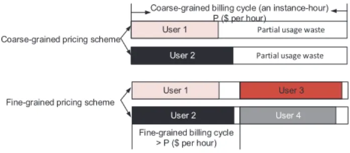
Such a phenomenon is called partial usage waste, which appears very often as cloud jobs are quite short in general [10]. Based on the recent characterization of Cloud environment versus Grid systems [10], cloud jobs are usually much shorter (such as dozens of min-utes) than Grid jobs (such as dozens of hours or days). This will induce serious partial usage waste issue. As illustrated in Fig. 1, the current hourly pricing scheme probably induce idle charged resources especially for short jobs, while the fine-grained pricing scheme not only makes users pay less but also makes provider gain more due to the optimization of unit price for the same service time and more users served.
Some highly skilled users aggregate their jobs into a long job [11] or unite with other users under a broker-age service [12], [13] to utilize the whole instance hour. But it either requires professional knowledge which is probably a little bit too hard for ordinary users, or
Partial usage waste
Partial usage waste
User 1
User 2
User 1
User 2
Coarse-grained billing cycle (an instance-hour) P ($ per hour)
Coarse-grained pricing scheme
Fine-grained pricing scheme
Fine-grained billing cycle > P ($ per hour)
User 4
User 3
Fig. 1: Users suffer from long partial usage waste in the coarse-grained pricing scheme, which can be largely reduced in the optimized fine-grained pricing scheme. Furthermore, the provider can gain more profit due to the higher unit price and serve more users in the optimized fine-grained pricing.
trusts other brokers whose credibilities can hardly be guaranteed.
Nowadays, once customers terminated the in-stances, some IaaS providers naturally take it for granted that they can get to reuse the resources imme-diately even if customers still charge the whole time period [2], [11]. It might be potential illegal because a seller cannot sell a single item (here the resource instance) to two customers, which is a violation in e-conomics [14]. And also this is unfair to the customers. A few other IaaS providers are trying to solve the partial usage waste issue by offering optional fine-grained pricing schemes. For example, CloudSigma [8] offers a Burst Pricing scheme that changes ev-ery five minutes upon busy-status. Google Compute Engine (GCE) [3] offers a 10-minutes based pricing scheme, in which all machine types are charged a minimum of 10 minutes. However, none of them identify and analyze the partial usage waste issue. This paper is the first attempt to quantitatively op-timize a fine-grained pricing scheme and investigate the optimization of the tradeoff between fine-grained pricing scheme and various overheads.
We highlight the main challenges and contributions of this paper as follows.
(1) Does the partial usage waste problem really exist in cloud environment and is it a significant problem? • Contribution 1:In the pay-as-you-go cloud pric-ing, short-job users have to pay more than what they actually use, and incur numerous idle in-stance time for the provider. We first raise the
partial usage waste issue [11], and then prove its significance by analyzing it with real-world production traces.
(2) How to optimize the tradeoff between adopting the refined pricing scheme and controlling the impact of extra overheads with decreasing length of billing cycles?
• Contribution 2: A VM instance’s maintenance cost like boot-up, shut-down, and dynamic tun-ing resource amounts, is often a relatively large constant, which means that shorter tasks will be more sensitive to the VM-maintenance cost.
We propose a novel optimized fine-grained fair pricing scheme by taking into account the VM-maintenance overhead, and find a best-fit billing cycle to reach the maximized social welfare (i.e., the sum of the cost reductions for all customers and the revenue gained by the provider). (3) How to coordinate the benefits of customers (or users) and providers by simply refining the time granularity such that both sides feel satisfied?
• Contribution 3: Intuitively, the profits of both sides contradict to each other, such that win-win status is hard to guarantee. We derive an optimal price point which can satisfy both users and providers with maximized total utility. Our scheme also proves that refined fine-grained pric-ing is not bad news for service providers, because they can keep or even increase their revenue with our scheme.
(4) What are the experimental results like when per-forming our optimized fine-grained pricing scheme using real-world production trace, as compared to the existing coarse-grained hourly pricing scheme?
• Contribution 4: We evaluate our new pricing scheme using a 1-month Google trace [15], [16] and a 22-months production DAS-2 trace [17] downloaded from Grid Workload Archive (GWA) [18]. Experimental results indicate that under our optimized fine-grained pricing scheme, for the DAS-2 (Google), the social welfare can be in-creased up to72.98% (48.15%).
For the remainder of the paper, we use the terms IaaS platform, IaaS cloud, and cloud environment interchangeably, and we also use the terms customer, consumer, and user interchangeably. In Section 2, we analyze the partial usage waste issue and describe our optimized fine-grained pricing model by taking into account the VM-maintenance overhead, as compared to the conventional cloud pricing scheme. We discuss in Section 3 our main algorithms in coordinating the profit from both sides and coping with the tradeoff between optimizing fine-grained pricing scheme and minimizing overheads. We carefully evaluate our so-lution and present the performance evaluation results in Section 4. In Section 5, we discuss some issues and future work. We discuss the related work in Section 6, and finally, conclude the paper in Section 7.
2
RESOURCE
PRICING
SCHEME
In this section, we first briefly review the existing clas-sic IaaS cloud pricing schemes, and then analyze the partial usage waste issue, and finally formulate our optimized fine-grained pricing model by taking VM-maintenance overhead into consideration. Our main objective is to satisfy both customers and providers, and reach maximum social welfare meanwhile.
2.1 Classic Cloud Pricing Schemes
In recent times, the pricing schemes broadly adopted in IaaS cloud market [2], [8], [19], [20], [21] can be categorized into three types: pay-as-you-go offer, subscription option and spot market. Under the pay-as-you-go scheme, users pay a fixed rate for cloud resource consumption per billing cycle (e.g., an hour) with no commitment. On-Demand Instances are often used to run short-jobs or handle periodic traffic spikes [2].
In the subscription scheme, users need to pay an upfront fee to reserve resources for a certain period of time (e.g., a month) and in turn receive a significant price discount. The billing cycles in the subscription scheme are relatively long compared to the pay-as-you-go scheme, and can be one day, one month, or even several years [22], [19], [20], [21]. Therefore, it is suitable for long-running jobs (like scientific computing [4]). A special example in this scheme is Amazon Reserved Instances [22], instances during the reserved period are charged hourly, but they are still not suitable for short-jobs due to the high upfront fee. For the spot scheme [23], users simply bid on spare instances and run them whenever their bid prices ex-ceed the current Spot Price. Spot Instances are suitable for time-flexible, interruption-tolerant tasks (like web-crawling or Monte Carlo applications) [23], because they can significantly lower the computing costs due to the extremely low Spot Price. But the drawback of Spot Instance is the instances can be terminated by the provider any time. Therefore, it is meaningless to exploit fine-grained billing cycle as the tasks are time-insensitive, even though the cost of a spot instance is also calculated based on one hour time unit.
Our paper focuses on the pay-as-you-go offer, which is especially suitable for short-running cloud jobs because of finer pricing granularity.
2.2 Analysis of Partial Usage Waste
VMs in pay-as-you-go pricing, for the example of on-demand instances in EC2, are recommended for applications with short term, spiky, or unpredictable workloads that cannot be interrupted (i.e., short-jobs) [2]. These VM instances are always charged hourly, yet short-job users have to pay for full hour cost even their jobs just consumed the resources with a small portion of the one-hour period. This phenomenon is calledpartial usage waste.
In order to quantify the partial usage waste issue, we introduce theinstance time utilizationmetric, which means the consumed time percentage in user’s pur-chased instance hours. However, workload traces in public clouds are often confidential: no IaaS cloud has released its usage trace so far. For this reason, we use a 1-month Google cluster-trace [15], [16] and a 22-months production DAS-2 trace [17] in our analysis. Although Google cluster is not a public IaaS cloud,
its usage traces can reflect the demands of Google engineers and services, which can represent demands of public cloud users to some degree. While the DAS-2 is a wide-area grid datacenter, its usage traces are slightly different from the cloud services. But the traces are still generated from real-life production system, which can represent the demands of potential cloud users in future.
Specially, in order to increase the representativeness of these data traces, we rule out the extremely short jobs (e.g., less than 1 minutes) because those very short jobs could be failed jobs that are corrected and resubmitted. After ruling out the outliers, we evaluate theinstance time utilizationfor every user in two traces and plot the results in Fig. 2. As indicated in Fig. 2, in the hourly pricing, majority of users in both traces get low (<20%) instance time utilizations, which implies a serious phenomenon of partial usage waste.
Though the workload traces in public clouds are confidential, the partial usage waste issue can be no-ticed in many research [24], [11], [12] in the literature of cloud computing. Juve et al. [24] ran workflow experiments on Amazons EC2 and noticed that the cost assuming per-hour charges is greater than the cost assuming per-second charges. Kouki et al. [11] used a strategy with an instance waiting for the end of an instance-hour to terminate can be useful if there is an increasing workload. The cost saving of as much as 30% can be achieved by using RightCapacity. Wang et al. [12] used the brokerage to exploit the partial usage and brought a cost saving of close to 15%.
Such partial usage waste not only makes users pay more than what they actually use, but also leads to skewness of the expected revenue from the perspec-tive of providers (to be discussed in details later).
2.3 Formulation of Fine-Grained Pricing Scheme In this paper, we propose a novel optimized fine-grained pricing scheme to solve the above issues. The objective of our work is two-fold, with regard to the classic coarse-grained pricing scheme and inevitable VM-maintenance overhead. On one hand, we aim to derive an acceptable pricing range for both customers and providers, and also derive an optimal price that satisfies both sides with maximized total utility. On the other hand, we hope to find a best-fit billing cycle to maximize the social welfare related to both sides.
There are three key terms in our fine-grained pric-ing scheme: resource bundle, time granularity and unit price. Theresource bundleserves as a kind of container to execute task workloads based on user demands. Thetime granularityis defined as the minimum length in pricing the rented resources. Theunit pricespecifies how much the user needs to pay per time granularity for the resource consumption. We give an example to illustrate the above terms. In Amazon EC2’s
pay-as-79.8%
16.7% 4.5%
Low Medium High
(a) DAS-2 79.8% 16.7% 4.5% 42.4% 41.4% 16.2%
Low Medium High
(b) Google
Fig. 2: Statistics of users’ instance time utilization in the hourly pricing. The users are spilt into three groups (i.e., Low Utilization group, Medium Utilization group and High Utilization group) based on different levels of instance time utilization. Users’ instance time utilization in Low group, Medium group, High group is [0, 20%), [20%, 80%), [80%, 100%] respectively. For example, 79.8% (42.4%) of users in DAS-2 (Google) get low (i.e.,<20%) instance time utilization.
you-go option, users need to pay $0.0441per hour for
a small on-demand VM instance (Unix/Linux usage). In this example, the VM instance which bundles CPU, RAM, data storage and bandwidth together is the resource bundle. The time granularity is one hour and the unit price is equal to $0.044. As another example, in CloudSigma [8], the resource bundle is not an instance but just some type of resource like CPU or RAM. CloudSigma does not bundle them together but allows customers to finely tune the combination of resources on demand exactly. Our work focuses on the time granularity and the unit price, aiming to imple-ment an optimized fine-grained pricing scheme with regard to VM-maintenance overhead like VM boot-up cost. For simplicity reasons, the cloud resource bundle mentioned in our paper is referred to as VM instance similar to EC2 on-demand instance.
Time granularity (i.e.,length of billing cycle, denoted asK in our model) is the major concern. The length of billing cycle is often relatively long under existing schemes. For example, in a pay-as-you-go scheme, the billing cycle is usually set to one hour, for the purpose of easing the management because such a coarse-grained pricing scheme with long-length billing cy-cle could neglect the impact of the VM-maintenance overhead to a certain extent. However, such an hourly pricing scheme suffers from serious partial usage waste, which can be resolved intuitively using an optimized fine-grained pricing scheme, where the key challenge is that VM-maintenance overhead will be fairly prominent with decreasing length of the billing cycle.
Unit price is another key term in our pricing model, and it is determined by the time unit (such as an hour) and the pricing unit with respect to the time unit (such as hourly pricing). The pricing unit is denoted byP($
1We use the price released on Amazon website [2] before 9th April, 2014.
per hour)in the hourly pricing. Suppose the billing cy-cle isK-minutes in our optimized fine-grained pricing scheme, the unit price is denoted as PK. Intuitively, the original payment under the hourly pricing scheme during a period of K-minutes can be computed as P(K−To)
60−To . In practice, however, the valid productive period of a VM instance is shorter than its real life-cycle because of inevitable VM-maintenance overhead like VM boot-up cost and VM resource amount tuning cost. Especially, provider’s gain should be guaranteed with no less profit than that in the coarse-grained pricing scheme for the same service time. Hence, PK in our optimized fine-grained pricing scheme is supposed to be no less than the original payment. That is,PK can be represented as Formula (1), where
χindicates an increment price (≥0).
PK =
P(K−To)
60−To
+χ. (1)
This increment priceχ can be used to not only cov-er providcov-ers’ loss due to VM-maintenance ovcov-erhead described below (details in Section 3.2) but also gain more profit for providers (details in Section 3.3).
The last concern is the VM-maintenance overhead like VM boot-up cost, task startup cost or operation time on VM resource allocation. In general, for a particular VM instance, these overheads are usually constants determined by the VM memory size [25], [26], [27]. We denote the VM-maintenance overhead byTo (evaluated by minutes), including VM bootup cost, resource allocation cost, and so on. Without loss of generality, we suppose To is too large to be ne-glected in fine-grained pricing scheme. For simplicity reasons, the overhead we assume is a constant, which conforms to reality for the given jobs. Because of the characterization of Google traces [28], the overhead is always related to the memory size, and the memory sizes of majority jobs are stable. Mao et al. [26]’s
char-acterization shows that booting up a new VM instance always suffers from To ≈ 96.9 seconds regardless of the length of billing cycle.
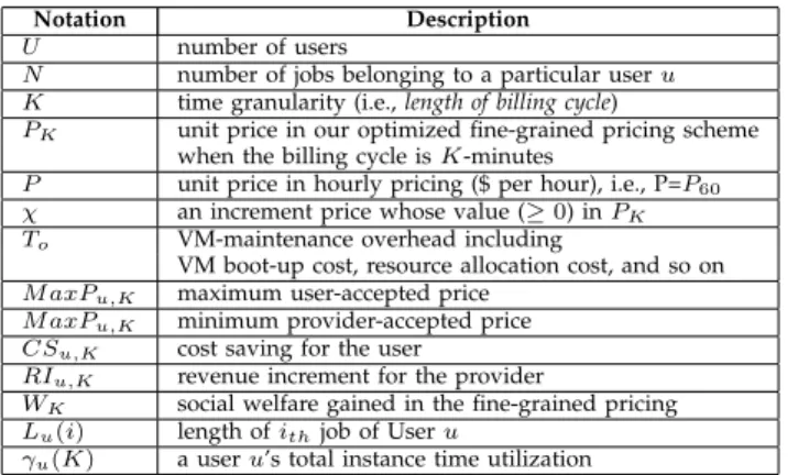
We summarize the key notations in Table 1. TABLE 1: Summary of Key Notations
Notation Description
U number of users
N number of jobs belonging to a particular useru K time granularity (i.e.,length of billing cycle)
PK unit price in our optimized fine-grained pricing scheme when the billing cycle isK-minutes
P unit price in hourly pricing ($ per hour), i.e., P=P60
χ an increment price whose value (≥0) inPK To VM-maintenance overhead including
VM boot-up cost, resource allocation cost, and so on
M axPu,K maximum user-accepted price
M axPu,K minimum provider-accepted price CSu,K cost saving for the user
RIu,K revenue increment for the provider
WK social welfare gained in the fine-grained pricing Lu(i) length ofithjob of Useru
γu(K) a useru’s total instance time utilization
3
OPTIMIZED
FINE-GRAINED
PRICING
AL-GORITHM
In this section, we optimize the fine-grained pricing scheme by proposing three algorithms with regarding to VM-maintenance overheads: computing maximum user-accepted price (denoted M axPu,K, whereuand
Kindicate user and billing cycle length respectively), computing minimum provider-accepted price
(denot-edM inPu,K), and maximizing the social welfare. With
these three algorithms, one can easily find a win-win state satisfying both users and providers as long as the final price is set in the acceptable pricing range
[M inPu,K, M axPu,K]. Then, we will prove that the
optimal price point is M inPu,K+M axPu,K
2 , which can maximize the overall satisfaction degree regarding both sides. Finally, we will find a best-fit billing cycle to maximize the social welfare.
3.1 Compute Maximum User-accepted Price Suppose a cloud provider has U different usersU , {1, 2,· · ·,U }. Each user payment will be investigated individually in our model. For a particular user u who has N jobs, we use Lu(i) to denote the length of the user’sithjob running on some cloud instances. Specially, if two conjoint jobs (i.e., user’sithandi+1th job) submit in the same billing cycle, they are deemed as one job.
When running a user’s jobs in cloud with the fine-grained billing cycle =K-minutes, the unit price PK is supposed to be higher than the original price value calculated based on hourly pricing, as Formula (1) shows.
In order to study the feasibility of our optimized fine-grained pricing scheme, we need to compute the total cost that can be accepted by users for all of their jobs, instead of the single cost for a particular job. The
total cost for useruwith billing cycle =K-minutes can be written as Formula (2), where⌈Lu(i)
K−To⌉indicates the number of billing cycles (a ceiling value) for the user’s ithjob in our optimized fine-grained pricing scheme.
Costu,K=PK N ∑ i=1 ⌈ Lu(i) K−To⌉ (2) Apparently, Costu,60 indicates the cost of user u running all of his/her jobs in the classic coarse-grained hourly pricing scheme. With the computation of Costu,K, we can compute the maximum price that can be accepted by users (denoted asM axPu,K) per billing cycle based on Formula (3) (when billing cycle =K-minutes). When a user’s task just runs for K minutes, the original payment under the coarse-grained pricing scheme will force him/her to pay the whole one-hour cost P. That is, our users will feel worthy as long as their final payments under our optimized fine-grained pricing scheme are no higher thanP.
M axPu,K= T otal P ayment under Coarsegrained pricing scheme#of cycles in the F inegrained pricing scheme
=P∑Ni=1 ⌈ Lu(i) 60−To ⌉/∑N i=1 ⌈ Lu(i) K−To ⌉ (3) The pseudo-code in computing the maximum prices for user u with the fine-grained billing cycle K-minutes is described in Alg. 1. The intuitive idea is to compute the maximum prices that can be accepted by the user u with respect to different fine-grained billing cycles.
Algorithm 1 Computing maximum price that can be accepted by users
Input: The lengthLu(i)of Useru’s all jobs.
Output: A vector which contains the maximum prices
M axPu,Kthat can be accepted by the user.
1: CalculateCostu,60for all of the user’s jobs with hourly pricing.
2: forall billing cycles Kdo
3: Calculate the total number of billing cycles for all ofu’s jobs based on the fine-grained pricing.
4: Calculate the value ofM axPu,K.
5: end for
In this algorithm, we first compute the original payment that the user can stand based on classic pric-ing scheme with coarse-grained rate. And then, we compute the maximum prices which can be accepted by the user for different lengths of billing cycles (line 3). The users will feel satisfied as long as their costs in our new pricing scheme are less or equal to the costs computed in the classic pricing scheme. Note that the coarse-grained pricing scheme forces the minimum billing cycle to be one hour (60 minutes), which means that the finally settled cost Costu,K should be no larger than Costu,60 in our optimized fine-grained scheme. In the following text, we will derive the minimum price that can be accepted by providers, and finally derive an optimal price point.
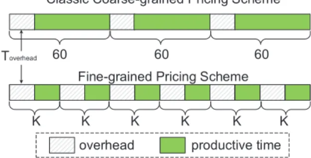
3.2 Compute Minimum Provider-accepted Price The designed optimized fine-grained pricing scheme should also satisfy providers, yet providers may suffer higher overhead due to finer pricing rates. In the classic coarse-grained pricing scheme, the provider will sufferToto manage VM instance every one hour service. In the optimized fine-grained pricing scheme, the provider may suffer higher overhead due to more frequent context switch among VM instances. We use an example to highlight the difference between the two pricing schemes in Fig. 3. Obviously, the provider will suffer higher loss of payment in the second pricing scheme with finer granularity due to more frequent VM overheads appearing in the whole service time.
Classic Coarse-grained Pricing Scheme
Fine-grained Pricing Scheme
overhead productive time
60 60 60
K K K K K K
Toverhead
Fig. 3: Service time analysis between two pricing schemes. As follows, we will derive the minimum acceptable price in the K-minutes billing cycle for the provider based on the VM overhead To in comparison to the classic coarse-grained pricing scheme. For the same service period with length = Tservice, we use m and
nto denote the number of billing cycles in the classic pricing scheme and that in our optimized fine-grained pricing scheme respectively. In the example shown in Fig. 3, m = 3 and n = 6. Then, it is easy to derive Equation (4) based on Fig. 3.
Tservice=m·60 =n·K (4) On the other hand, the minimum price accepted by the provider is reached when the provider’s total gains in the new pricing scheme is equal to the payment earned in the classic pricing scheme, i.e., Equation (5), whereP refers to the price in the classic hourly pricing scheme.
m·P =n·M inPK (5)
Based on Equation (4) and Equation (5), we can get Formula (6).
M inPK =
K
60·P (6)
Together with Formula (1), we can get Formula (7). χoverhead=M inPK−
P(K−To)
60−To
(7)
Obviously,χoverhead is the increment price to over-come the overhead in our optimized fine-grained pricing scheme. The pseudo-code of the algorithm in computing the minimum provider-accepted prices for different lengths of billing cycles is similar to Alg. 1. What need to do is just replacingM axPu,KbyM inPK and removing the computation ofCostu,K.
3.3 Optimal Price in the Acceptable Range In this part, we derive the optimal price value dur-ing the range ([M inPu,K, M axPu,K]) derived above, which is accepted by both users and providers. Before analysis, we need to define the satisfaction function for both users and providers.
As shown in Fig. 4, we model the user/provider satisfaction based on the utility theory in economics. According to [14], the utility function is concave, which shows how utility, a subjective measure of satisfaction, depends on wealth. We use price to take the place of wealth in the X-Axis because the wealth in this paper is proportional to the price. Meanwhile, the wealths of the user and the provider are symmetric because the reduction of provider’s wealth will be gained by the user in turn. Hence, the two utility functions (belonging to user and provider respective-ly) are both concave and symmetric with respect to the middle point minPu,K+2maxPu,K.
0 MinP (MinP+MaxP)/2 MaxP Price Axis User utility function
f(MinP+MaxP-x)
Provider utility function f(x) Utility
Umax
Fig. 4: Utility functions and optimal price point. It is obvious that if the provider’s utility function is denoted by f(x), then the user’s utility function can be denoted byf(M inP+M axP−x). We use the summation of the two utility values with respect to a particular price xto denote the total utility (denoted as F(x)), as shown in the following formula. Then, the optimal price point is supposed to maximize the total utilityF(x)regarding the both participants (user and provider).
F(x) =f(x) +f(minP +maxP−x) (8)
Theorem 1: For the acceptable range [MinP,MaxP], the optimal price point x∗ for maximizing the total utility (or satisfaction) is equal to M inP+2M axP.
Proof: Since f(x) is concave, we have ∂2f(x)
∂2f(M inP+M axP−x)
∂x2 < 0. Then,
∂2F(x)
∂x2 < 0. That is,
the value of F(x) has a maximum point during the range [MinP,MaxP], and F(x)reaches the maximum value when ∂F∂x(x) = 0.
Then, we can derive the optimal price point as follows: ∂F(x) ∂x = ∂f(x) ∂x + ∂f(M inP+M axP−x) ∂x
= ∂f∂x(x)−∂f∂y(y) = 0, where y=M inP+M axP−x
This leads to ∂f∂x(x) =
∂f(y)
∂y , where
y=M inP+M axP−x. Obviously, this equation holds
if and only if the price valuex=M inP+2M axP. That is, x∗=M inP+M axP
2 .
Similarly to Formula (7), with the optimal price M inP+M axP
2 , we can get Formula (9). χoptimal=
M inPK+M axPu,K
2 −
P(K−To)
60−To (9) Obviously, χoptimal will be larger than χoverhead
when M axPu,K is larger than M inPK. The value
χoptimal −χoverhead is the increment price to gain more revenue with the same service time billed in the optimized fine-grained pricing scheme for the provider. Specially, it is possible thatM inPKis greater
thanM axPu,K when the billing cycle is short and the
impact of VM-maintenance cannot be neglected, just like the situation illustrated in Fig. 9(a).
3.4 Discussion of Social Welfare Maximization Up to now, we have discussed how to derive an optimal price in the acceptable range to satisfy both users and providers with maximized total utility. We will discuss the social welfare gained in our optimized fine-grained pricing scheme.
Social welfare WK includes the cost saving CSu,K for all users and revenue increment RIu,K for the provider. WK = U ∑ u=1 CSu,K+ U ∑ u=1 RIu,K (10)
Specially,RIu,K>0 means that the provider can gain more profit by the same service time billed in the fine-grained pricing scheme than that in the old scheme. As the billing cycle goes from2minutes to60minutes,
M axPu,K and M inPK changes separately, and so
does the social welfare. There should exist a best-fit billing cycle to obtain a maximum social welfare, we denote it asBF, as illustrated in Alg. 2.
In this algorithm, we first compute the total cost that the user costs in the hourly pricing scheme and our optimized fine-grained pricing scheme for differ-ent lengths of billing cycles. Users obtain cost saving when the cost in classic hourly pricing scheme is higher than the cost in our optimized pricing scheme (line 4). The provider gains revenue increment when the cost for the same service time billed in the fine-grained pricing scheme is higher than that billed in
Algorithm 2 Maximize Social Welfare
Input: The maximum priceM axPu,Kfor the useru; The minimum
priceM inPK for the provider.
Output: The maximum social welfare M axW and the best-fit
billing cyclesBF.
1: Calculate the total cost Costu,60 for all jobs in the hourly
pricing.
2: forall billing cycles Kdo
3: Calculate the total cost Costu,K for all jobs in our
op-timized fine-grained pricing scheme with optimal price
M inPK+M axPu,K
2 .
4: CSu,K ←
Costu,60−Costu,K
Costu,60 . /* Cost saving for useru*/
5: RIu,K←
Costu,K/K−Costu,60/60
Costu,60/60 . /* Compute the revenue
increment for provider */
6: end for
7: forall users at billing cycle Kdo
8: Calculate the social welfare WK for all users and the
provider.
9: end for
10: Select the maximum social welfareM axW=WKm, when the
billing cycle isKm. 11: BF←Km.
the classic hourly pricing scheme (line 5). And then, we calculate the social welfare over different lengths of billing cycles (line 7-9), and find a best-fit billing cycle point for social welfare maximization (line 8). 3.5 Algorithm Complexity
In Algorithm 1, for a given User u, calculating the Costu,60costsO(N), and calculatingM axPu,K for all billing cyclesK costsO(KN). For all users,
calculat-ing M axPu,K is O(U)∗O(N+KN)). Thus the time
complexity of Algorithm 1 isO(U KN). In Algorithm 2, calculating for social welfare also costsO(KN)for a given Useru. Thus the time complexity of Algorithm 2 is alsoO(U KN).
4
PERFORMANCE
EVALUATION
In this section, we conduct simulations driven by a large volume of real-world traces to evaluate the fea-sibility of our optimized fine-grained pricing scheme, with an extensive range of scenarios.
4.1 Experimental Setting
We use a 1-month Google cluster trace [15], [16] and a 22-months production DAS-2 trace [17] in our exper-iments. Google trace involves over 370,000 valid jobs running across over 12,000 hosts from a Google data center. There are about 4000 applications in total, such as Mapreduce programs [29] and other data-mining programs. Each job contains one or more tasks, and there are totally 25 million tasks in the trace. The DAS-2 trace contains 300+ users with over 1 million jobs. The VM overhead is simulated based on Mao et al.’s characterization over real cloud environment [26]:To ≈96.9 seconds.
We will present the experimental results about in-stance time utilization, maximum user-accepted price,
minimum provider-accepted price, and social welfare maximization respectively. We compare the results under our optimized fine-grained pricing scheme and the classic coarse-grained one in the experiments. The best-fit billing cycle is also investigated.
4.2 Evaluation of Instance Time Utilization A user u’s total instance time utilization (denoted as γu(K)) is determined by running all of his/her jobs with an assigned billing cycle =K-minutes. The com-putation of γu(K) is shown in Formula (11), where ⌈Lu(i)
K−To⌉indicates the number of billing cycles (a ceil-ing value) for the user’sithjob in our optimized fine-grained pricing scheme.
γu(K) = ∑N i=1Lu(i) K∑Ni=1⌈KLu−(Ti) o⌉ . (11)
The instance time utilization is a subjective measure of partial usage waste as discussed in Section 2.2. Appar-ently, the lower instance time utilization a user gets, the more seriously partial usage waste he/she suffers. The overall instance time utilization with billing cycle K in the whole system can be denoted by such a vectorγ(K),(γ1(K), . . . , γU(K)).
We simulate the resource charging based on lengths of jobs with different instances and various billing cy-cles, and compute the instance time utilization based on Formula (11).
Fig. 2 presents the statistical results about the in-stance time utilizations in DAS-2 system and Google data center in the hourly-rate pricing scheme (i.e., classic coarse-grained pricing scheme). In this situa-tion, the billing cycle is always set to one hour (K = 60 minutes). We can clearly observe that the users can be split into three groups based on different levels of instance time utilization.
• Group 1 (Low Utilization): The utilization of the users in this group is lower than20%.
• Group 2 (Medium Utilization): The utilization of the users in this group is between20%and 80%. • Group 3 (High Utilization): The utilization of the
users in this group is higher than80%.
In principle, different groups of users will benefit from our optimized fine-grained pricing scheme to different extents: the lower utilization in the classic pricing scheme, the higher social welfare earned in our fine-grained pricing scheme.
In the following text, we intensively investigate the optimized fine-grained pricing scheme. For simplicity, we set the time resolution of billing cycle to one minute, i.e., the smallest billing cycle in our experi-ment is one minute. Our evaluations are carried out for each group.
We present the instance time utilizations with d-ifferent billing cycles in Fig. 5, in which all partial usages are billed as full billing cycles. We draw the
2 5 10 15 20 25 30 35 40 45 50 55 60 0 20 40 60 80 100
Billing cycle (Min)
Instance time utilization (%)
Group 3 (DAS−2) Group 3 (Google) Group 2 (DAS−2) Group 2 (Google) Group 1 (DAS−2) Group 1 (Google)
Fig. 5: The utilization curves with different billing cycles for three groups.
instance time utilization curves for each group of users (showing the average values of randomly se-lected users in each group) in the figure. It is clearly observed that the average instance time utilizations of the three groups (low/medium/high-utilization) are about 10%, 42%, 90% for DAS-2 and about 10%, 63%, 91% for Google trace in the hourly pricing. When the billing cycle is set to 2 minute, the instance time uti-lizations reach highest point for different groups, from 70-100% for both traces. This means a huge advantage in using fine-grained pricing scheme compared to the coarse-grained pricing scheme.
We observe that most of jobs gain a lot instance u-tilization improvement in our optimized fine-grained pricing scheme. In absolute terms, the optimized fine-grained pricing scheme for low-utilization jobs achieves the improvement by about 71%
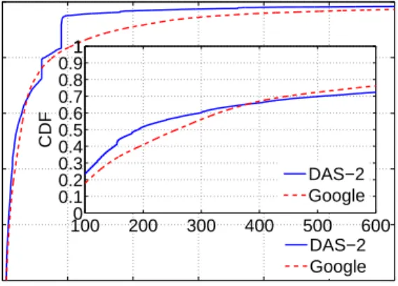
10%≈7 times for both traces. This is due to the fact that the majority of job lengths are fairly short (about several or dozens of minutes). We present the cumulative distribution function (CDF) of the job lengths for Google and
DAS-2in Fig. 6. It is observed that over70%of both traces’ jobs are shorter than 600 seconds even though we have ruled out the extremely short jobs.
0 1000 2000 3000 4000 5000 6000 0 0.2 0.4 0.6 0.8 1
Job length (Seconds)
CDF 1000 200 300 400 500 600 0.1 0.2 0.3 0.4 0.5 0.6 0.7 0.8 0.911 CDF DAS−2 Google DAS−2 Google
4.3 Evaluation of Social Welfare
To evaluate how much social welfare can be gained in our optimized fine-grained pricing scheme, we need to check two bound prices: The maximum price which can be accepted by users (described in Section 3.1) and the minimum price which can be accepted by the provider (described in Section 3.2), then we can use Alg. 2 to compute the social welfare achieved in our optimized fine-grained pricing scheme.
4.3.1 Maximum User-accepted Price
We evaluate the maximum prices which can be accept-ed by all users over different billing cycles as follows. Prices are normalized with respect to hourly pricing. As defined previously, the hourly price is denoted as P, then the price for a K-minutes billing cycle is PK. We normalize price for PK to be PK/P /(60(K−−TTo)
o). When the billing cycle is 60 minutes (i.e., the same as the hourly pricing), the normalized price (i.e., P) is 1. We evaluate our optimized fine-grained pricing
1 1.1 1.2 Group 3 1 2 3 Group 2
Maximum user−accepted price (Normalized to hourly pricing)
2 5 10 15 20 25 30 35 40 45 50 55 60 0
10 20
Group 1 Billing cycle (Min)
Das−2 Google Das−2 Google Das−2 Google
Fig. 7: The maximum user-accepted prices with different billing cycles.
schemes for the three groups and plot the results in Fig. 7. There are two findings observed through the figure. First, as expected, we can see that the prices for users from Group 3 are less than the ones from Group 2 and far less than that from Group
1. The reason is that users in Group 1 have very short jobs, and short jobs will cause large number of partial usage wastes in hourly pricing. Second, the price for shorter billing cycle is always higher because shorter billing cycle leads to less partial usage waste. However, some anomalous situations appear in Fig. 7 (e.g., the line segment from 25 to 30 in the middle figure for Google). The reason for this unusual result is that the users in Group 2 (Google) have very few jobs and many jobs are close to the long billing cycle. This may lead to less waste in a slightly longer billing cycle.
4.3.2 Minimum Provider-accepted Price
From the provider’s perspective, we need to eval-uate the minimum price which can be accepted
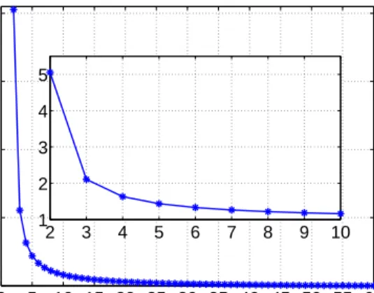
by provider in our optimized fine-grained pricing scheme. We compute the minimum provider-accepted using Formula 4, which is described in Section 3.2. Similarly, we also normalize this minimum provider-accepted price to the hourly price, and plot the results in Fig. 8. From the figure we can see, as the billing cycle goes from2minute to60minutes, the minimum provider-accepted price drops sharply from 5.05 to
1. That is because the value of overhead time To in Formula (12) will not change in different billing cycles.
0 5 10 15 20 25 30 35 40 45 50 55 60 1 2 3 4 5
Billing cycle (Min)
Minimum provider−accepted price (Normalized to hourly pricing)
2 3 4 5 6 7 8 9 10 1 2 3 4 5
Fig. 8: The minimum provider-accepted price caused by overhead. We represent the extra costVodue to VM overhead by Formula (12). That is,Vodenotes the price value of the VM overheads like VM startup cost in the hourly price.
Vo=
To
60P. (12)
If the billing cycle is very short, the impact of the overheadVo will be significant. In contrast, when the billing cycle is very long (e.g.,50minutes), the impact of value Vo will be tiny. The normalized minimum provider-accepted price will be 1 when the billing cycle is 60 minutes (i.e., the hourly pricing).
4.3.3 Users Cost Saving
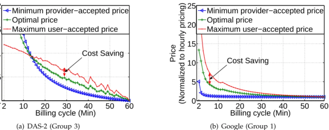
As described in Section 4.3, the social welfare includes cost saving for users and revenue increment for the provider. We now evaluate the cost saving for users with the optimal price described in Section 3.3. We plot the result in Fig. 9.
In Fig. 9, we only plot the result of Group 3 users in DAS-2 and Group 1 users in Google. The other group users have similar figures. Cost saving for the user is the part where the maximum user-accepted price is higher than the optimal price. For example, in Fig. 9(b), the maximum user-accepted prices of the users are always higher than the optimal price. But for the users in Group3 in Fig. 9(a), cost saving only happens when the billing cycles are longer than 14
minutes. That is, when the billing cycle is shorter than14 minutes, there will be no cost saving in our optimized fine-grained pricing scheme for Group3.
2 10 20 30 40 50 60 1 1.05 1.1 1.15 1.2
Billing cycle (Min)
Price
(Normalized to hourly pricing)
Minimum provider−accepted price Optimal price
Maximum user−accepted price
Cost Saving
(a) DAS-2 (Group 3)
2 10 20 30 40 50 60 0 5 10 15 20 25
Billing cycle (Min)
Price
(Normalized to hourly pricing)
Minimum provider−accepted price Optimal price
Maximum user−accepted price
Cost Saving
(b) Google (Group 1) Fig. 9: The cost saving for the Group 3 users in DAS-2 and Group 1 users in Google.
4.3.4 Provider Revenue Increment
We evaluate the revenue increment with the optimal price for the provider as described in Alg. 2 and plot the result in Fig. 10. Compared to the hourly pricing, the provider needs less service time to complete the users’ workload in the fine-grained pricing due to the reduction of partial usage waste. We define the resource saturation ratio by dividing the service time needed in the fine-grained pricing by the service time needed in the hourly pricing. From Fig. 10, we see that, in the fine-grained pricing, the provider only needs to spend 36.78% (42.24%) of the service time needed in the hourly pricing and gains 94.10%
(73.75%) of the revenue gained in the hourly pricing for DAS-2 (Google). That is to say, the resource is unsaturated in the fine-grained pricing due to the reduction of partial usage waste.
The provider’s resource can serve more customers in the fine-grained pricing. If more customers come into the cloud and the provider’s resource is sat-urated, the provider will gain more revenue than that in hourly pricing due to the higher unit price and more users served. As we observe, the revenue gained by the provider will reach up to 255.85%
(174.60%) when the provider’s resource is saturated (i.e., 100% of the service time needed in the hourly pricing) for DAS-2 (Google). That is, the providers’ revenue can be guaranteed in our optimized fine-grained pricing. Their revenue can be even increased (to what extents depending on the saturation of the resource), which can effectively motivate providers to continually charge resources with our optimized fine-grained pricing.
4.3.5 Social Welfare Maximization
We then evaluate the most significant contribution of this paper, the best-fit billing cycle to gain social welfare maximization. It seems that the shorter the billing cycle is, the more social welfare gains. But the evaluation results show that it is not so, as illustrat-ed in Fig. 11. The maximum social welfare 72.98%
Unsaturated Saturated Unsaturated Saturated 0 50 100 150 200 250 300
Compared to the hourly pricing (%)
Service time Revenue Google DAS−2 100% 100% 174.60% 255.85% 36.78% 94.10% 73.75% 42.24%
Fig. 10: Compared to hourly pricing, less service time is needed to complete the same users’ workload (Unsaturated) and less revenue gained by the provider in our optimized fine-grained pricing. But billing the same service time (Saturated) as in hourly pricing, the provider will gain more revenue in our optimized fine-grained pricing. 2 5 10 20 30 40 50 60 −100 −50 0 50 100
Billing cycle (Min)
Social welfare (%)
Das−2 Google
72.98%
48.15%
Fig. 11: The social welfare with different billing cycles.
(48.15%) is reached when the billing cycle is5minutes (9minutes) for DAS-2 (Google), which is equivalent to the best-fit billing cycle for DAS-2 (Google), but not the other shorter billing cycles. That is because the social welfare comes from the increasing utilization in the new pricing scheme, while billing in shorter cycle will incur higher overhead. It is worth noting that the social welfare appears to be negative for
Google users when the billing cycle is shorter than
3 minutes. That is to say, with those billing cycles, Google users will get no social welfare in the new pricing scheme, obviously, these billing cycles are not suitable for Google users.
4.3.6 Fixed Fine-grained Billing Cycle
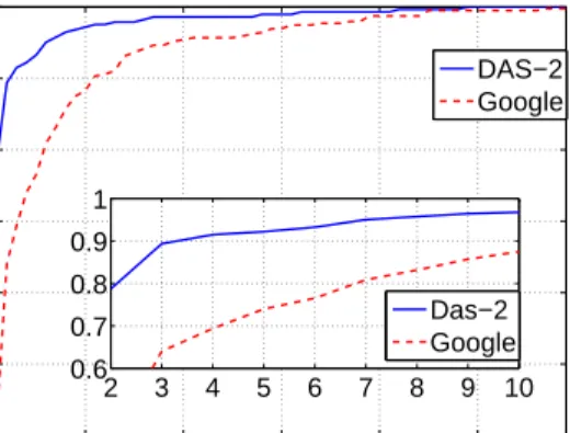
Up to now, we have evaluated the best-fit billing cycle for social welfare maximization, but the best-fit billing cycle is not suitable for all users, as mentioned in Fig. 9(a), the best-fit billing cycle 5-minutes is not suitable for Group 3 users in DAS-2. It seems that the billing cycle needs to be dynamic. However, many vendors and users like to be more stable and predictable, which needs a fixed billing cycle. We evaluate the feasibility of the fixed billing cycle in this part. In Fig. 12, we plot the CDF of users who can accept the billing cycles in the X-axis. For a given Y-minutes billing cycle, if the cost savingCSu,K=Y of Useruis greater than 0, then we believe that User u can accept the Y-minutes billing cycle. Because users cannot accepted a new price to complete the same workload with a higher cost.
2 10 20 30 40 50 60 0.4 0.5 0.6 0.7 0.8 0.9 1
Billing cycle (Min)
CDF 2 3 4 5 6 7 8 9 10 0.6 0.7 0.8 0.9 1 DAS−2 Google Das−2 Google
Fig. 12: Distribution of users which can accept the billing cycles in fine-grained pricing scheme.
From Fig. 12, we see that, nearly 80% of users in DAS-2 can accept 2-minutes as the billing cycle, but only 40% of users in Google. Meanwhile nearly 80% (90%) of users in Google can accept 5-minutes (10-minutes) as the billing cycle.
We suggest that 5-minutes is a proper fixed billing cycle for the IaaS provider for several reasons. First, the social welfare at 5-minutes billing cycle is almost the same as the maximization for both traces as illus-trated in Fig. 9. Second, the5-minutes billing cycle can be accepted by most users in both traces as illustrated in Fig. 12.
5
DISCUSSIONS
In this section, we will discuss several issues that have not yet been investigated above.
5.1 Benefits for IaaS Market
Intuitively, the profits of both users and providers contradict to each other, because the provider’s total revenue may reduce as the existence of cost savings for users in our optimized fine-grained pricing. There-fore how do customers and providers benefit from our optimized fine-grained pricing?
Benefits for Cloud Customers: Apparently, short-job users will get cost saving in the fine-grained pricing scheme due to the reduction of partial usage waste.
Benefits for Service Providers: First, the revenue increment presented in Section 4.3 means that the rev-enue gained by the provider for the same service time will increase in our optimized fine-grained pricing. Second, when more and more customers rush into the cloud [1], providers will gain more revenue due to the higher unit price in the fine-grained pricing. Third, in our simulation, we derive the optimal price to satisfy both sides. In reality, providers can be more flexible. For example, the provider can attract more customers by leaving a portion of the revenue to customers, or get more revenue by taking a portion of the cost saving from customers. Finally, as GCE [3] and many other IaaS providers [2], [8], [19] emerge, the competition among them will be more and more severe and cruel. Providers with fine-grained pricing scheme, like GCE, can be more competitive to survive, due to their attractive and precise pricing method to customers.
Towards Perfect IaaS Market:The IaaS cloud mar-ket is flourishing more and more, which has attracted a large number of customers from different domains. But the reality is that the marketplace today is an oligopoly, not aperfect market[30] with a large number of suppliers. The idea proposed in our paper can encourage new services providers to come up with and offer optimized fine-grained pricing scheme to start competing with the existing dominant providers. Conversely, the existing providers will need to con-sider this prospect and be willing to start offering competitive pricing to prevent competition growth. They will probably loose out if they do not offer a competitive pricing scheme. Therefore, our work has a chance to improve the IaaS market.
5.2 Other Potential Benefits of Fine-Grained Pric-ing
The proposed fine-grained pricing scheme in this paper is mainly suitable for short-running cloud jobs. Actually, there are some benefits of fine-grained pric-ing even for long-runnpric-ing jobs. For example, in the coarse-grained pricing, customers have to be more conservative, because they will lose much money tearing down and up VMs all the time. But the fine-grained pricing allows them to release VMs more elastically after load lowers. As another example,
suppose a service wants to segregate subsets of its users into different VMs for some security purpose. Maybe they will consider doing that in the context of the more flexible pricing, but not in the context of the coarse-grained one. Those will be discussed and investigated in our future work.
6
RELATED
WORK
Some work discussed how to take advantage of the existing cloud pricing schemes to reduce running cost [31], [32], [33], [11] in the perspective of the IaaS users. Hong et al. [31], for example, designed a strategy with on-demand instance to reduce the margin costs
and another strategy combining the on-demand and reserved instance to reduce the true costs. Zhao et al. [32] leveraged EC2 Spot Price Prediction to design a resource renting strategy to reduce the cost of cloud applications. Moreover, many work just wanted to deconstruct and debunk the truth of Spot pricing scheme, and leveraged it to reduce users’ cost [33]. Kouki et al. [11] had realized the existence of partial usage waste, and learned to terminate an instance at the end of an instance-hour. While our work not only proves the significance of the partial usage waste, but also utilizes it to gain more revenues by designing a fine-grained pricing.
Some other work [12], [13], [34], [35] utilized a third party (e.g., IaaS cloud broker) to connect customers and providers of computing sources. For example, Wang et al. [12] proposed a broker that aggregates on-demand instances and reserved instances to serve users, while users’ behavior resembles launching in-stances on demand provided by the broker. Similarly, Niu et al. [13] proposed a Semi-Elastic Cluster com-puting model for organizations to reserve and resize a virtual cloud-based cluster. SpotCloud [34] provided the world’s first global market for cloud capacity, buy-ing and sellbuy-ing unused computbuy-ing capacity globally is available. Song et al. [35] proposed a broker to bid for Spot Instance with EC2 Spot Price Prediction and used them to serve cloud users. Shanmuganathan et al. [36] implemented the software prototype as part of VMware’s management for tenants to flexibly multi-plex their purchased capacity dynamically among its VMs. All these work made decisions either from the perspective of users or providers but not both, while our approach satisfies both sides simultaneously in fine-granularity.
Some existing work [37], [7], [38], [39] also tried to compromise the profits of users and providers, yet they did not consider the impact of VM overheads in fine-grained pricing scheme. Di et al. [37] proposed a win-win cloud scheduling method by leveraging the second-first price policy, in order to reach a win-win status with strategy proof. Ben-Yehuda et al. [7] pro-posed a brief overview of a new cloud, which is called as Resource-as-a-Service (RaaS) clouds. Sharma et al.
[38] proposed a financial economic model for pricing cloud compute commodities. They discuss the results for four different metrics to guarantee the quality of service. Haas et al. [39] proposed a formal economic model for a co-operative infrastructure for a socially oriented platform and analyzed the feasibility and scalability of the model. To the best of our knowledge, we are the first to explore an optimized fine-grained pricing scheme for IaaS cloud.
Dynamic pricing with respect to the market forces [9], [40], [41] is a hot topic in the literature. Xu et al. [9] designed an optimal dynamic pricing policy, with the presence of stochastic demand and perishable resources, so that the expected long-term revenue is maximized. Ardagna et al. [40] modeled the service provisioning problem as a generalized Nash game and proposed two solution methods based on the best-reply dynamics. CloudPack* [41] was proposed to optimize the use of cloud resources to minimize total costs while allocating clients’ workloads to reach a game-theoretic fairness. These approaches are com-plementary to our fine-grained pricing, which can be studied with our approach in the future.
In summary, compared to the existing work, there are many advantages in adopting our optimized fine-grained pricing scheme: (1) our fine-fine-grained pricing scheme is fairly flexible to suit various types of ser-vices and spiky demands raised by users, unlike the coarse-grained hourly pricing scheme; (2) our fine-grained pricing scheme can effectively reduce the partial usage waste because the idle instance time can be allocated to more customers especially in a competitive situation; (3) Users will feel more satisfied due to the more precise computation of the payment cost, such that more users will join the cloud and resource providers can also benefit in turn.
7
CONCLUSION AND
FUTURE
WORK
This paper takes the first step to identify and study the partial usage waste issue in cloud computing by analyzing its significance with real-world traces. We propose an optimized fine-grained pricing to solve the partial usage waste issue, with regard to the inevitable VM-maintenance overhead, and find a best-fit billing cycle to maximize the social welfare. By applying the utility theory in economics, we derive an optimal price (the middle point in the range) to satisfy both customers and providers with maximized total utili-ty. We evaluate our optimized pricing scheme using two large-scale production traces (based on DAS-2 and Google), with comparison to the classic coarse-grained hourly pricing scheme. Maximum social wel-fare can be increased up to 72.98% and 48.15% with respect to DAS-2 trace and Google trace respectively. The following research issues are planned for the future work. First, our approach mainly focuses on the IaaS provider’s perspective but not the users’
perspective. In the future, we will explore a dynamic solution to cope with the changing demands of users and providers.
Second, the design of pricing can be affected by the market forces due to the competitiveness among resource providers. Our approach has not considered the influence on pricing caused by the market forces. We plan to exploit the best-fit auction based policies to suit the new fine-grained pricing scheme in the future. Third, the partial usage waste problem can be al-leviated by scheduling users’ jobs effectively. In the future, we plan to investigate a pipeline solution for the partial usage waste problem combined with users’ scheduling knowledge.
ACKNOWLEDGMENT
We would like to thank the anonymous reviewers for their insights and comments that help us improve the quality of this paper. We would like to thank the Ad-vanced School for Computing and Imaging (the own-er of DAS-2 system), and the Grid Workload Archive, and Google Inc for making their invaluable data traces available. The research is supported by National Sci-ence Foundation of China under grant No.61232008, National 863 Hi-Tech Research and Development Pro-gram under grant No.2013AA01A213, Chinese Uni-versities Scientific Fund under grant No.2013TS094, Research Fund for the Doctoral Program of MOE un-der grant No.20110142130005, and EU FP7 MONICA project under grant No.295222.
REFERENCES
[1] R. Stefan, K. Holger, M. Pascal, B. Andrew, and L. Miroslaw, “Sizing the cloud,” Forrester Research, 2011.
[2] Amazon Elastic Compute Cloud. [Online]. Available: http://aws.amazon.com/ec2/
[3] Google Compute Engine. [Online]. Available: https://cloud.google.com/pricing/compute-engine
[4] E. Deelman, G. Singh, M. Livny, G. B. Berriman, and J. Good, “The cost of doing science on the cloud: the Montage ex-ample,” in Proceedings of the International Conference on High Performance Computing, Networking, Storage and Analysis (SC), 2008.
[5] A. Marathe, R. Harris, D. Lowenthal, B. Supinski, B. Rountree, M. Schulz, and X. Yuan, “A comparative study of high-performance computing on the cloud,” in Proceedings of the 22nd ACM International Symposium on High Performance Dis-tributed Computing (HPDC), 2013.
[6] S. Di and C.-L. Wang, “Error-tolerant resource allocation and payment minimization for cloud system,” IEEE Transactions on Parallel and Distributed Systems (TPDS), vol. 24, no. 6, pp. 1097–1106, 2013.
[7] O. Agmon Ben-Yehuda, M. Ben-Yehuda, A. Schuster, and D. T-safrir, “The resource-as-a-service (raas) cloud,” inProceedings of the 4th USENIX conference on Hot Topics in Cloud Computing (HotCloud’12), 2012, pp. 12–12.
[8] CloudSigma. [Online]. Available: http://www.cloudsigma.com/
[9] H. Xu and B. Li, “Dynamic cloud pricing for revenue maxi-mization,”IEEE Transactions on Cloud Computing (TCC), vol. 1, no. 2, pp. 158–171, 2013.
[10] S. Di, D. Kondo, and W. Cirne, “Characterization and compari-son of cloud versus grid workloads,” inInternational Conference on Cluster Computing (CLUSTER), 2012, pp. 230–238.
[11] Y. Kouki and T. Ledoux, “Rightcapacity: Sla-driven cross-layer cloud elasticity management,”IJNGC, vol. 4, no. 3, 2013. [12] W. Wang, D. Niu, B. Li, and B. Liang, “Dynamic cloud resource
reservation via cloud brokerage,” in IEEE 33nd International Conference on Distributed Computing Systems (ICDCS), 2013. [13] S. Niu, J. Zhai, X. Ma, X. Tang, and W. Chen, “Cost-effective
cloud hpc resource provisioning by building semi-elastic vir-tual clusters,” inProceedings of the International Conference on High Performance Computing, Networking, Storage and Analysis (SC), 2013, p. 56.
[14] G. Mankiw, “Principles of economics,” Sourth-Western Pub, 2008.
[15] More Google cluster data, google re-search blog, nov. 2011. [Online]. Avail-able: http://googleresearch.blogspot.com/2011/11/more-google-cluster-data.html
[16] C. Reiss, J. Wilkes, and J.-L. Hellerstein. (Nov. 2011) Google cluster-usage traces: format + schema.
[17] Grid computing on das-2. [Online]. Available: http://www.cs.vu.nl/das2/das2-grid.html
[18] Grid workloads archive website. [Online]. Available: http://gwa.ewi.tudelft.nl/pmwiki/pmwiki.php?n=Workloads.Gwa-t-1
[19] Elastichosts. [Online]. Available: http://www.elastichosts.com/
[20] VPS.NET. [Online]. Available: http://vps.net
[21] GoGrid Cloud Hosting. [Online]. Available: http://www.gogrid.com
[22] Amazon EC2 Reserved Instances. [Online]. Available: http://aws.amazon.com/ec2/reserved-instances/
[23] Amazon EC2 Spot Instances. [Online]. Available: http://aws.amazon.com/ec2/spot-instances/
[24] G. Juve, E. Deelman, K. Vahi, G. Mehta, B. Berriman, B. P. Berman, and P. Maechling, “Data sharing options for scientific workflows on amazon ec2,” inProceedings of the International Conference on High Performance Computing, Networking, Storage and Analysis (SC), 2010, pp. 1–9.
[25] D. Gupta, L. Cherkasova, R. Gardner, and A. Vahdat, “Enforc-ing performance isolation across virtual machines in xen,” in Proceedings of 7th ACM/IFIP/USENIX Int’l Conf. on Middleware (Middleware), 2013, pp. 342–362.
[26] M. Mao and M. Humphrey, “A performance study on the vm startup time in the cloud,” in2012 IEEE Fifth International Conference on Cloud Computing, 2012, pp. 423–430.
[27] Z. Hill, J. Li, M.Mao, A. Ruiz-Alvarez, and M. Humphrey, “Early observations on the performance of windows Azure,” inProceedings of the 19th ACM International Symposium on High Performance Distributed Computing (HPDC), 2010.
[28] S. Di, Y. Robert, F. Vivien, D. Kondo, C.-L. Wang, and F. Cap-pello, “Optimization of cloud task processing with checkpoint-restart mechanism,” inProceedings of the International Conference on High Performance Computing, Networking, Storage and Analy-sis (SC), 2013, pp. 64:1–64:12.
[29] J. Dean and S. Ghemawat, “MapReduce: Simplified data processing on large clusters,” in5th USENIX Symposium on Operating Systems Design and Implementation (OSDI), 2004, pp. 137–150.
[30] G. Mankiw, “Principles of microeconomics,” Sourth-Western Pub, 2008.
[31] Y.-J. Hong, J. Xue, and M. Thottethodi, “Dynamic server provi-sioning to minimize cost in an iaas cloud,” inProceedings of the ACM SIGMETRICS/international conference on Measurement and modeling of computer systems (SIGMETRICS), 2011, pp. 147–148. [32] H. Zhao, M. Pan, X. Liu, X. Li, and Y. Fang, “Optimal resource rental planning for elastic applications in cloud market,” in IPDPS, 2012, pp. 808–819.
[33] O. Agmon Ben-Yehuda, M. Ben-Yehuda, A. Schuster, and D. Tsafrir, “Deconstructing amazon ec2 spot instance pricing,” ACM Transactions on Economics and Computation (TEAC), vol. 1, no. 3, p. 16, 2013.
[34] SpotCloud. [Online]. Available: http://spotcloud.com/ [35] S. Yang, Z. Murtaza, and L. Kang-Won, “Optimal bidding in
spot instance market,” inProf. of IEEE Infocom, 2012. [36] G. Shanmuganathan, A. Gulati, and P. Varman,
“Defragment-ing the cloud us“Defragment-ing demand-based resource allocation,” in Proceedings of the ACM SIGMETRICS/international conference on
Measurement and modeling of computer systems (SIGMETRICS), 2013, pp. 67–80.
[37] S. Di, C.-L. Wang, and L. Chen, “Ex-post efficient resource allocation for self-organizing cloud,”Journal of Computers and Electrical Engineering (CEE), 2013.
[38] B. Sharma, R. K. Thulasiram, P. Thulasiraman, S. K. Garg, and R. Buyya, “Pricing cloud compute commodities: A novel financial economic model,” in 12th IEEE/ACM International Symposium on Cluster, Cloud and Grid Computing (ccgrid 2012), 2012, pp. 451–457.
[39] C. Haas, S. Caton, K. Chard, and C. Weinhardt, “Co-operative infrastructures: An economic model for providing infrastruc-tures for social cloud computing,” inSystem Sciences (HICSS), 2013 46th Hawaii International Conference on, Jan 2013, pp. 729– 738.
[40] D. Ardagna, B. Panicucci, and M. Passacantando, “Generalized nash equilibria for the service provisioning problem in cloud systems,”Services Computing, IEEE Transactions on, vol. 6, no. 4, pp. 429–442, Oct 2013.
[41] V. Ishakian, R. Sweha, A. Bestavros, and J. Appavoo, “Cloud-pack* exploiting workload flexibility through rational pric-ing,” in Proceedings of the 13th International Middleware Con-ference (Middleware ’12), 2012, pp. 374–393.
Hai Jinis a Cheung Kung Scholars Chair Professor of computer science and engineer-ing at Huazhong University of Science and Technology (HUST) in China. He is now Dean of the School of Computer Science and Technology at HUST. Jin received his PhD in computer engineering from HUST in 1994. In 1996, he was awarded a German Academic Exchange Service fellowship to visit the Technical University of Chemnitz in Germany. Jin worked at The University of Hong Kong between 1998 and 2000, and as a visiting scholar at the University of Southern California between 1999 and 2000. He was awarded Excellent Youth Award from the National Science Foundation of China in 2001. Jin is the chief scientist of ChinaGrid, the largest grid computing project in China, and the chief scientists of National 973 Basic Research Program Project of Virtualization Technology of Computing System, and Cloud Security.
Jin is a senior member of the IEEE and a member of the ACM. He has co-authored 15 books and published over 500 research papers. His research interests include computer architecture, virtualization technology, cluster computing and cloud computing, peer-to-peer computing, network storage, and network security.
Xinhou Wangis currently a Ph.D. candidate student in Service Computing Technology and System Lab (SCTS) and Cluster and Grid Lab (CGCL) at Huazhong University of Science and Technology (HUST) in China. His research interests include optimization of distributed resource allocation on cloud computing and virtualization.
Song Wu is a Professor of Computer Sci-ence at Huazhong University of SciSci-ence and Technology (HUST) in China. He received his Ph.D. from HUST in 2003. He is now served as the Director of Parallel and Distributed Computing Institute, and the Vice Head of Service Computing Technology and System Lab (SCTS) of HUST. He has published more than one hundred papers and obtained over twenty patents in the area of parallel and distributed computing. His current research interests include cloud resource scheduling, system virtualization and large-scale datacenter management.
Sheng Di received his master degree (M.Phil) from Huazhong University of Sci-ence and Technology in 2007 and Ph.D degree from The University of Hong Kong in 2011. He is currently a post-doctor re-searcher at Argonne National Laboratory (USA). His research interest is optimization of distributed resource allocation and fault-tolerance for Cloud Computing and High Performance Computing. His background is mainly on the fundamental theoretical analy-sis and system implementation.
Xuanhua Shireceived his Ph.D. degree in Computer Engineering from Huazhong Uni-versity of Science and Technology (HUST) in 2005. From 2006, he worked as an INRIA Post-Doc in PARIS team at Rennes for one year. Currently he is an associate profes-sor in Service Computing Technology and System Lab (SCTS) and Cluster and Grid Computing Lab (CGCL) at Huazhong Univer-sity of Science and Technology (China). His research interests include cluster and grid computing, fault-tolerance, web services, network security and grid security, virtualization technology, data-intensive computing. He is a member of the IEEE.