Kernelized Supervised
Dictionary Learning
by
Mehrdad Jabbarzadeh Gangeh
A thesis
presented to the University of Waterloo in fulfillment of the
thesis requirement for the degree of Doctor of Philosophy
in
Electrical and Computer Engineering
Waterloo, Ontario, Canada, 2013
c
I hereby declare that I am the sole author of this thesis. This is a true copy of the thesis, including any required final revisions, as accepted by my examiners.
Abstract
The representation of a signal using alearned dictionary instead ofpredefinedoperators, such as wavelets, has led to state-of-the-art results in various applications such as denoising, texture analysis, and face recognition. The area of dictionary learning is closely associated with sparse representation, which means that the signal is represented using few atoms in the dictionary. Despite recent advances in the computation of a dictionary using fast algorithms such as K-SVD, online learning, and cyclic coordinate descent, which make the computation of a dictionary from millions of data samples computationally feasible, the dictionary is mainly computed using unsupervised approaches such as k-means. These approaches learn the dictionary by minimizing the reconstruction error without taking into account the category information, which is not optimal in classification tasks.
In this thesis, we propose a supervised dictionary learning (SDL) approach by incorpo-rating information on class labels into the learning of the dictionary. To this end, we pro-pose to learn the dictionary in a space where the dependency between the signals and their corresponding labels is maximized. To maximize this dependency, the recently-introduced Hilbert Schmidt independence criterion (HSIC) is used. The learned dictionary is compact and has closed form; the proposed approach is fast. We show that it outperforms other unsupervised and supervised dictionary learning approaches in the literature on real-world data.
Moreover, the proposed SDL approach has as its main advantage that it can be eas-ily kernelized, particularly by incorporating a data-driven kernel such as a compression-based kernel, into the formulation. In this thesis, we propose a novel compression-compression-based (dis)similarity measure. The proposed measure utilizes a 2D MPEG-1 encoder, which takes into consideration the spatial locality and connectivity of pixels in the images. The proposed formulation has been carefully designed based on MPEG encoder functionality. To this end, by design, it solely uses P-frame coding to find the (dis)similarity among patches/images. We show that the proposed measure works properly on both small and large patch sizes on textures. Experimental results show that by incorporating the pro-posed measure as a kernel into our SDL, it significantly improves the performance of a supervised pixel-based texture classification on Brodatz and outdoor images compared to
other compression-based dissimilarity measures, as well as state-of-the-art SDL methods. It also improves the computation speed by about 40% compared to its closest rival.
Eventually, we have extended the proposed SDL to multiview learning, where more than one representation is available on a dataset. We propose two different multiview approaches: one fusing the feature sets in the original space and then learning the dictionary and sparse coefficients on the fused set; and the other by learning one dictionary and the corresponding coefficients in each view separately, and then fusing the representations in the space of the dictionaries learned. We will show that the proposed multiview approaches benefit from the complementary information in multiple views, and investigate the relative performance of these approaches in the application of emotion recognition.
Acknowledgements
All the praises and thanks are to God who gave me the strength and knowledge to accomplish this research.
Writing this thesis was not possible without support of my highly esteemed supervisors Dr. Mohamed Kamel and Dr. Ali Ghodsi. They both assisted me through many interesting technical conversations, offered guidance, and made suggestions that helped make my research work better. I would also like to express my gratitude to my Ph.D. committee: Dr. Ling Guan, Dr. Paul Fieguth, Dr. Otman Basir, and Dr. Zhou Wang, for providing valuable feedback and comments on my thesis.
I am very grateful for support and suggestions from many colleagues at University of Waterloo, especially in the Center for Pattern Analysis and Machine Intelligence (CPAMI), including Aya Sayedelahl, Pouria Fewzee, Ahmed Farahat, Pooyan Khajehpour, Rodrigo Araujo, Mike Miao Yun-Qian, Abbas Ahmadi, Michael Diu, Amir Hossein Shabani, Hossein Parsaei, Babak Alavi-Kia, Sepideh Seifzadeh, Kaushik Roy, Farook Sattar, Fatemeh Dorri, Nabil Drawil, and Yibo Zhang.
This research was financially supported by the Natural Sciences and Engineering Re-search Council (NSERC) and also the Ontario Ministry of Training, Colleges and Uni-versities. This support made it also possible for me to visit the Pattern Recognition Lab at Delft University of Technology in the Netherlands, where I was thrilled by their high-quality research work. I especially enjoyed having technical discussions with Dr. Robert P.W. Duin, Marco Loog, David Tax, and Laurens van der Maaten.
I gratefully acknowledge the joint work with: Lauge Sørensen and Marleen de Bruijne from the Dept. of Computer Science, Copenhagen University, Denmark; Saher B. Shaker from the Department of Respiratory Medicine, Gentofte University Hospital, Hellerup, Denmark; and Ali Sadegji Naini and Dr. Gregory Czarnota from the Dept. of Radiation Oncology and Imaging Research, Sunnybrook Health Sciences Center, Canada.
A research work cannot be accomplished without highly-qualified support staff. I’d like to express my appreciation to Ms. Rosalind Klein, the secretary of the CPAMI, and all other supporting staff at the ECE for their caring and kind administrative support.
I thank very much my parents for their unconditional love and kindness, and my brother and sisters for their encouragement and good wishes during my Ph.D.
Last but not least, special thanks to my wife, Maryam, for her love, patience, en-couragement, and support during my research, and to my sons, Ali and Iman, for their understanding and also for giving joy and happiness to my life.
Dedication
Table of Contents
List of Tables xi
List of Figures xiii
List of Abbreviations xv
1 Introduction 1
1.1 Related Topics . . . 2
1.2 Taxonomy of DLSR . . . 3
1.3 Objectives and Contributions . . . 4
1.4 Organization . . . 5
2 Literature Review 7 2.1 Unsupervised Dictionary Learning . . . 7
2.2 Supervised Dictionary Learning . . . 9
2.2.1 Learning One Dictionary per Class . . . 9
2.2.2 Pruning Large Dictionaries . . . 13
2.2.5 Including Category Information in the Learning of the Sparse
Coef-ficients . . . 18
2.2.6 Learning a Histogram of Dictionary Elements over the Signal Con-stituents . . . 20
3 Proposed Supervised Dictionary Learning 26 3.1 Hilbert Schmidt Independence Criterion . . . 27
3.2 Supervised Dictionary Learning Formulation . . . 29
3.3 Proposed Kernelized SDL . . . 33
4 Experiments on the Proposed SDL and KSDL 36 4.1 Implementation Details . . . 36
4.2 Face Data . . . 40
4.3 Digit Recognition . . . 41
4.4 Other Real-World Data . . . 45
4.5 Computation Cost of the Proposed SDL . . . 47
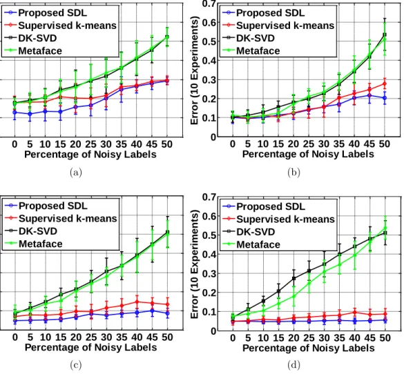
4.6 The Effect of Noisy Labels on the Performance of the Proposed SDL. . . . 53
5 Data-Dependent Kernels 57 5.1 Introduction . . . 57
5.2 Normalized Information Distance . . . 58
5.3 Normalized Compression Distance . . . 59
5.4 1D vs. 2D Compressors. . . 60
5.5 Proposed Compression-Based Similarity Measure . . . 61
5.5.1 Some Illustrative Results on Textures . . . 63 5.6 Kernelized Supervised Dictionary Learning Using Data-Dependent Kernels 64
5.6.1 Texture Classification on Stationary Images . . . 67
5.6.2 Pixel-Based Texture Classification on Nonstationary Images . . . . 68
5.7 Summary . . . 70
6 Extension of the Proposed SDL to Multiview Representations 73 6.1 Introduction . . . 73
6.2 Multiview Supervised Dictionary Learning . . . 74
6.3 Multiview SDL in Facial Expression Recognition . . . 78
6.3.1 Datasets . . . 80
6.3.2 Facial Features . . . 83
6.3.3 Implementation Details . . . 84
6.3.4 Results . . . 85
6.4 Multiview SDL in Speech Emotion Recognition (SER) . . . 88
6.4.1 Datasets . . . 91
6.4.2 Audio Features . . . 93
6.4.3 Implementation Details . . . 95
6.4.4 Results . . . 96
6.5 Summary . . . 98
7 Conclusions and Future Work 101 7.1 Summary and Conclusion . . . 101
7.2 Future Work . . . 104
7.3 List of Publications . . . 105
List of Tables
4.1 The datasets used in this chapter. . . 37 4.2 Classification error (E) and balanced error (BE) on test set for Olivetti face
data using the proposed SDL. . . 42 4.3 Classification error on test set for digit recognition on USPS data using
proposed SDL. . . 45 4.4 The results of classification error (%) on Sonar, Ionosphere, and Texture
datasets. . . 48 4.5 The results of classification balanced error (%) on Sonar and Ionosphere
datasets. . . 49 4.6 The results of classification error (%) on Heart, Parkinsons, and Satimage
datasets. . . 50 4.7 The results of classification balanced error (%) on Heart, Parkinsons, and
Satimage datasets. . . 51 4.8 The average computation time per fold (in seconds) on Sonar and Heart
datasets. . . 53 5.1 Classification error and the number of nonzero coefficients on the test set
for texture pair D5-D92 of Brodatz album. . . 69 5.2 The classification rate (%) compared among the proposed method and other
6.1 Face emotion datasets used in the experiments. . . 82
6.2 Classification accuracy (%) of facial expression recognition system based
on single-view (SV) and multiview (MV) supervised dictionary learning ap-proaches.. . . 87
6.3 Balanced classification accuracy (%) of facial expression recognition system
for CK+ and VAM datasets. . . 88
6.4 The average time (in seconds) over each fold for the single-view and
multi-view FER systems. . . 89 6.5 The percentage ofcorrelation coefficient (r) of the speech expression
recog-nition system based on single-view (SV) and multiview (MV) supervised dictionary learning approaches. . . 98
6.6 The computation time (in seconds) for the single-view and multiview SER
List of Figures
1.1 Topics related to and the applications of dictionary learning and sparse representation. . . 3 2.1 The illustration of two steps of a texton-based system. . . 21 2.2 Taxonomy of dictionary learning and sparse representation approaches. . . 25 4.1 Typical face images from the Olivetti face dataset in two classes of glasses
vs. no-glasses. . . 41 4.2 The dictionaries learned at the dictionary size of two on the Olivetti Face
dataset for (a) unsupervised k-means, (b) unsupervised K-SVD, (c) pro-posed SDL, (d) DK-SVD, (e) supervised k-means, and (f) metaface. . . 43 4.3 The error rate of the classification system for Olivetti face recognition system. 56 5.1 The distances computed on patches extracted from D4 and D5 of Brodatz
album. . . 65 5.2 The distances computed on patches extracted from two more texture pairs
from the Brodatz album. . . 66 5.3 Texture images of D5 and D92 from Brodatz album.. . . 68 5.4 The results of supervised pixel-based texture classification on Brodatz and
outdoor images. . . 72 6.1 Sample images from six face emotion classes for CK+ and JAFFE datasets. 81
6.2 Sample frames from four subjects of Vera Am Mittag (VAM) dataset. . . . 82 6.3 (a) A speech signal (b) SED component for q= 1, and (c) SED component
List of Abbreviations
1D One Dimensional 2D Two Dimensional
AIB Agglomerative Information Bottleneck AVEC Audio/Visual Emotion Challenge
BL Bilinear
BP Basis Pursuit
BSS Blind Source Separation
CCA Canonical Correlation Analysis CFA Cross-Modal Factor Analysis CK+ Extended Cohn-Kanade DCT Discrete Cosine Transform DK-SVD Discriminative K-SVD
DLSI Dictionary Learning with Structured Incoherence DLSR Dictionary Learning and Sparse Representation FCSC Fully-Continuous Sub-Challenge
FDDL Fisher Discrimination Dictionary Learning FER Facial Expression Recognition
FMF Facial Measure Features GMM Gaussian Mixture Model HNR Harmonic-to-Noise Ratio
HSIC Hilbert Schmidt Independence Criterion IB Information Bottleneck
JAFFE Japanese Female Facial Expression JPEG Joint Photographic Experts Group KL Kullback-Leibler
LASSO Least Absolute Shrinkage and Selection Operator LBP Local Binary Pattern
LLD Low-Level Description MAP Maximum A Posteriori
MFCC Mel Frequency Cepstrum Coefficients MKL Multiple Kernel Learning
MLE Maximum Likelihood Estimation MPEG Moving Picture Experts Group
MV Multiview
NCD Normalized Compression Distance NED Normalized Entropy-rate Distance NID Normalized Information Distance NNMF Nonnegative Matrix Factorization OMP Orthogonal Matching Pursuit RBF Radial Basis Function
RCF Randomized Clustering Forest SAL Sensitive Artificial Listener SC Sparse Coding
SCPO Self-describing Content-based Pixel Ordering SDL Supervised Dictionary Learning
SDL-D Supervised Dictionary Learning-Discriminative SDL-G Supervised Dictionary Learning-Generative SDLM Supervised Dictionary Learning Model SED Spectral Energy Distribution
SER Speech Emotion Recognition SIFT Scale Invariant Feature Transform
SRC Sparse Representation-based Classification
SVM Support Vector Machine SVR Support Vector Regression
UAV Universal and Adapted Vocabulary UVD Universal Visual Dictionary
Chapter 1
Introduction
There are many mathematical models to describe data with varying degrees of success, among which dictionary learning and sparse representation (DLSR) has attracted the in-terest of many researchers in various fields. Dictionary learning and sparse representation are two closely-related topics that have roots in the decomposition of signals to some pre-defined bases, such as the Fourier transform. Representation of signals using prepre-defined bases is based on the assumption that these bases are general enough to represent any kind of signal, however, recent research shows that learning the bases1 from data, instead of using off-the-shelf ones, leads to state-of-the-art results in many applications [1]. In fact, what makes DLSR distinct from the representation using predefined bases is that first, the bases are learned here from the data, and second, only a few components in the dictionary are needed to represent the data (sparse representation). This latter attribute can also be seen in the decomposition of signals using some predefined bases such as wavelets [2].
1Here, the term basis is loosely used as the dictionary can be overcomplete, i.e., the number of dictionary
elements can be larger than the dimensionality of the data, and its atoms are not necessarily orthogonal and can be linearly dependent.
1.1
Related Topics
The concept of dictionary learning and sparse representation originated in different com-munities attempting to solve different problems, which are given different names. Some of them are: sparse coding (SC), which was originated by neurologists as a model for sim-ple cells in mammalian primary visual cortex [3]; independent component analysis (ICA), which was developed by researchers in signal processing to estimate the underlying hidden components of multivariate statistical data (refer to [4] for a review of ICA); least absolute shrinkage and selection operator (lasso), which was used by statisticians to find linear re-gression models when there are many more predictors than samples, where some constraints have to be considered to fit the model. In thelasso, one of the constraints introduced by Tibshirani was the`1-norm that led to sparse coefficients in the linear regression model [5].
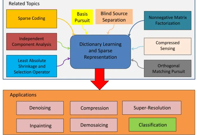
Another technique which also leads to DLSR is nonnegative matrix factorization (NNMF), which aims to decompose a matrix to two nonnegative matrices, one of which can be con-sidered to be the dictionary, and the other the coefficients [6]. In NNMF, usually both the dictionary and coefficients are sparse [6,7]. This list is not complete, and there are variants for each of the above techniques, such as blind source separation (BSS) [8], compressed sensing [9], basis pursuit (BP) [10], and orthogonal matching pursuit (OMP) [11,12]. It is beyond the scope of this thesis to include the description of all these techniques (interested readers can refer to [1,13–15] for reviews on dictionary learning and sparse representation). The main results of all these research efforts is that a class of signals with sparse nature, such as images of natural scenes, can be represented using some primitive elements that form a dictionary, and that each signal in this class can be represented by using only a few elements in the dictionary, i.e., by a sparse representation. In fact, there are at least two ways in the literature to exploit sparsity [16]: first, using a linear/nonlinear combination of some predefined bases, e.g., wavelets [2]; second, using primitive elements in a learned dictionary, such as the techniques employed in SC or ICA. This latter approach is the focus of this thesis and has led to state-of-the-art results in various applications such as texture classification [17–19], face recognition [20–22], image denoising [23,24], biomedical tissue characterization [25–27], motion and data segmentation [28,29], data representation and column selection [30], and image super-resolution [31]. Figure 1.1 summarizes the topics
Dictionary Learning and Sparse Representation Sparse Coding Independent Component Analysis Least Absolute Shrinkage and Selection Operator Nonnegative Matrix Factorization Compressed Sensing Orthogonal Matching Pursuit Denoising Inpainting Classification Compression Demosaicing Super-Resolution Applications Related Topics Basis Pursuit Blind Source Separation
Figure 1.1: Topics related to and the applications of dictionary learning and sparse repre-sentation.
related to and the applications of dictionary learning and sparse representation.
1.2
Taxonomy of DLSR
One may categorize the various dictionary learning with sparse representation approaches proposed in the literature in different ways: one where the dictionary consists of predefined or learned bases as stated above, and the other based on the model used to learn the dictio-nary and coefficients. These models can begenerative as used in the original formulation of SC [3], ICA [4], and NNMF [6]; reconstructive as in thelasso [5]; or discriminative such as
SDL-D (supervised dictionary learning-discriminative) in [16]. The two former approaches do not consider the class labels in building the dictionary, while the last one (i.e., the dis-criminative one) does. In other words, dictionary learning can be performed unsupervised or supervised, with the difference that in the latter, the class labels in the training set are used to build a more discriminative dictionary for the particular classification task in hand.
1.3
Objectives and Contributions
The main objectives of this thesis are as follows:
• To develop a supervised dictionary learning (SDL) algorithm by incorporating class labels into the learning of the dictionary;
• To design and incorporate a compression-based dissimilarity measure into the de-signed SDL as a kernel to further improve the discrimination power of the algorithm in subtle classification tasks;
• To extend the proposed SDL to multiview representations.
As the result of the research carried out, a novel supervised dictionary learning is proposed in this thesis by incorporating information on class labels into the learning of the dictionary. The dictionary is learned in a space where the dependency between the data and their corresponding labels is maximized. It is proposed to maximize this dependency by using the recently introduced Hilbert Schmidt independence criterion (HSIC) [32,33]. Although supervised dictionary learning has been proposed by others, as will be reviewed in the next chapter, this work is different from the others in the following aspects:
1. The formulation is simple and straightforward;
2. The proposed approach introduces a closed form formulation for the computation of the dictionary. This is different from other approaches, in which the computa-tion of diccomputa-tionary and sparse coefficients has to be iteratively and often alternately performed, which causes high computational load;
3. The approach is very efficient in terms of dictionary size (compact dictionary). The results show that the proposed dictionary can produce significantly better results than other supervised dictionary methods for small dictionary sizes. An important special case is when the dictionary size is smaller than the dimensionality of data. This turns the learning of a dictionary whose size is usually larger than the dimensionality of the data, i.e., an overcomplete dictionary, into the learning of asubspace;
4. The proposed approach can be easily kernelized by incorporating a kernel into the formulation. For example, data-dependent kernels based on normalized compression distance (NCD) [34,35], can be used in this kernelized SDL to further improve the discrimination power of the designed system. To the best of my knowledge, no other kernelized SDL approach has been proposed in the literature yet, and none of the proposed SDLs in the literature can be kernelized in a straightforward way.
A novel compression-based dissimilarity measure, particularly designed for textures, is also proposed. It is shown how it can be incorporated into the proposed kernelized SDL as a data-dependent kernel to significantly improve the accuracy of a pixel-based texture classification systems on benchmark datasets, such as the Brodatz album.
Eventually, the proposed SDL is extended to multiview representations. There are situations where there are more than one view/representation for a dataset. An effective way is proposed to make use of the complementary information available in all these rep-resentations, by learning one dictionary per view and computing the corresponding sparse coefficients. By fusing these coefficients, a multiview representation is provided where clas-sification can be performed faster and more accurately. The effectiveness of this multiview SDL in emotion recognition applications will be also shown .
1.4
Organization
The organization of the rest of the thesis is as follows: Chapter 2provides an overview on dictionary learning and sparse representation (DLSR). It first provides the formulation for
unsupervised dictionary learning, then extensively reviews many of the current supervised dictionary learning approaches in the literature and their shortcomings.
Chapter 3 provides the mathematical formulation for the proposed supervised dictio-nary learning approach. To this end, it first reviews the mathematical background for the proposed SDL, i.e., Hilbert Schmidt independence criterion (HSIC). Then provides the formulation for the proposed SDL and its kernelized version.
Chapter 4 presents the experimental setup and results on various datasets and in dif-ferent applications such as face recognition, digit recognition, and texture classification.
The proposed compression-based dissimilarity measure and its properties are described in Chapter5. This chapter first reviews the normalized information distance (NID) and its computable version, i.e., normalized compression distance (NCD). Then the formulation for the proposed measure is provided. Finally, it shows how by incorporating the proposed measure into the kernelized version of SDL, the performance of a texture classification system can be significantly improved.
Chapter6extends the proposed SDL to multiview and regression problems. The former is useful in applications where data is represented using more than one feature set, whereas the latter is needed when the information category is defined in continuous domain rather than a discrete one. The chapter shows the effectiveness of the proposed extensions to emotion recognition applications using speech and visual expressions. Finally, Chapter 7 concludes the thesis.
Chapter 2
Literature Review
In this chapter, an overview of the dictionary learning and sparse representation is provided. Also a brief review of recent attempts to make the approach more suitable for classification tasks is presented.
2.1
Unsupervised Dictionary Learning
Considering a finite training set of signals X = [x1,x2, ...,xn] ∈ Rp×n, where p is the
dimensionality and n is the number of data samples, according to classical dictionary learning and sparse representation (DLSR) techniques (refer to [1,13,14] for a recent review on this topic), these signals can be represented by a linear decomposition over a few dictionary atoms by minimizing a loss function as given below
L(X,D,α) =
n
X
i=1
l(xi,D,α), (2.1)
whereD ∈Rp×k is the dictionary of k atoms, and α∈
Rk×n are the coefficients.
This loss function can be defined in various ways based on the application in hand. However, what is common in DLSR literature is to define the loss function L as the
reconstruction error in a mean-squared sense, with a sparsity-inducing function ψ as a regularization penalty to ensure the sparsity of coefficients. Hence, (2.1) can be written as
L(X,D,α) = min D,α 1 2kX−Dαk 2 F+λψ(α), (2.2)
where subscript F indicates the Frobenius norm andλis the regularization parameter that affects the number of nonzero coefficients.
An intuitive measure of sparsity is `0-norm, which indicates the number of nonzero
elements in a vector1. However, the optimization problem obtained from replacing sparsity-inducing function ψ in (2.2) with `0 is nonconvex, and the problem is NP-hard (refer
to [14] for a recent comprehensive discussion on this issue). There are two main proposed approximate solutions to overcome this problem: the first is based on greedy algorithms, such as the well-known orthogonal matching pursuit (OMP) [11,12,14]; the second works by approximating a highly discontinuous `0-norm by a continuous function such as the
`1-norm. This leads to an approach which is widely known in the literature as lasso [5] or
basis pursuit (BP) [10], and (2.2) converts to
L(X,D,α) = min D,α n X i=1 1 2kXi−Dαik 2 F+λkαik1 . (2.3)
whereαi is the ith column of α.
In (2.3), the main optimization goal for the computation of the dictionary and sparse coefficients is minimizing the reconstruction error in the mean-squared sense. While this works well in applications where the primary goal is to reconstruct signals as accurately as possible, such as in denoising, image inpainting, and coding, it is not the ultimate goal in classification tasks [36], as discriminating signals is more important here. Hence, recently, there have been several attempts to include category information in computing either dictionary, coefficients, or both. In the following section, a brief overview of proposed supervised dictionary learning approaches in the literature will be provided. To this end, the proposed approaches are categorized into six different categories, while it is admitted that this taxonomy of approaches is not unique and could be done differently.
1`
2.2
Supervised Dictionary Learning
As mentioned in the previous section, (2.3) provides a reconstructive formulation for com-puting the dictionary and sparse coefficients, given a set of data samples. Although the problem is not convex on both dictionaryD and coefficientsα, this optimization problem is convex if it is solved iteratively and alternately on these two unknowns. Several fast algorithms have recently been proposed for this purpose, such as K-SVD [37], online learn-ing [38], and cyclic coordinate descent [39]. However, none of these approaches takes into account the category information for learning either the dictionary or the coefficients.
2.2.1
Learning One Dictionary per Class
The first and simplest approach to include category information in DLSR is computing one dictionary per class, i.e., using the training samples in each class to compute part of the dictionary, and then composing all these partial dictionaries into one. In providing the mathematical formulation for all the approaches in this category of SDL, it is always assumed that the training samples are grouped based on the classes they belong to such that X= [X1,X2, ...,Xc]∈Rp×n, wherec is the number of classes andXi = [xi1,xi2, ...,xim]∈
Rp×m is the group of training samples in class i.
Supervised k-means
Perhaps the earliest work in this direction is the one based on the so-called texton-based approach [19,40–44]. The texton-based approach, can be considered a dictionary learning approach particularly tailored for texture analysis. In this approach, textons, which are computed using the k-means clustering algorithm over patches extracted from texture images, play the role of dictionary atoms. Although in a texton-based approach the texture images are usually modeled with a histogram of textons and hence, the approach falls mainly into the category of supervised dictionary learning explained in Subsection 2.2.6, the idea of using k-means and the computed cluster centers as the dictionary elements can still be considered here as a SDL approach that computes one dictionary per class.
Therefore, a specific name is suggested for this technique, i.e., supervised k-means, to differentiate it from a texton-based approach. In supervised k-means, k-means is applied to the training samples in each class, and the k cluster centers computed are considered to be the dictionary for this class. These partial dictionaries are eventually composed into one dictionary.
In the mathematical framework, each subdictionary Di = [di1,di2, ...,diki]∈R
p×ki can
be computed using the training samples in class i, i.e., usingXi = [xi1,xi2, ...,xim]∈Rp×m
and the optimization problem
arg min Di ki X l=1 X xij∈Sl kxij −dilk (2.4)
whereS ={S1, S2, ..., Ski}areki clusters that partition data samplesXi in classi. Usually,
ki, the number of dictionary atoms computed per class, is the same over all classes. By
composing allDiinto one dictionary such thatD = [D1,D2, ...,Dc]∈Rp×k, wherek =ki·c,
the whole dictionary is obtained.
One can explain why it might be expected that a supervisedk-means performs better than an unsupervised one by understanding how k-means compute the cluster centers: it essentially computes the cluster centers by taking the mean of the points. Hence, if k -means was applied to the data points across classes, the resultant cluster centers might not be corresponding to the data points in any of the classes, and consequently the resultant cluster centers would not be identified uniquely with individual classes. In other words, the cluster centers computed usingk-means across classes would not be representing data samples in a class properly. Thus, in classification tasks, it will be beneficial, particularly at small dictionary sizes, to usek-means for the data points in one class at a time.
Sparse representation-based classification (SRC)
In [21], the training samples are used as the dictionary in face recognition and hence, this technique, called sparse representation-based classification (SRC), effectively falls into the same category as training one dictionary per class. However, no actual training is performed here, and the whole training samples are used directly in the dictionary.
To describe SRC more formally, suppose that xts ∈ Rp is a test sample. The SRC
algorithm assigns the whole training set X to the dictionary D, and computes the sparse coefficients α for test sample xts using the lasso given in (2.3) as follows
min α 1 2kxts−Xαk 2 2+λkαk1. (2.5)
In the next step, the residual error is computed for the reconstruction of the test sample using training samples of each class and their corresponding sparse coefficients
ri(xts) =kxts−Xδi(α)k22, (2.6)
where δi is a characteristic function that selects the coefficients associated with class i.
This residual error is found for each class separately, and then the class label of the given test samples is assigned according to
label(xts) = arg min
i
ri(xts). (2.7)
However, using the training samples as the dictionary in this approach results in a very large and possibly inefficient dictionary, due to the noisy training instances.
Metaface
To obtain a smaller dictionary, Yang et al. proposed an approach called metaface, which learns a smaller dictionary for each class and then composes them into one dictionary [45]. Metaface was originally proposed for the application of face recognition, but it is general and can be used in any application. In this approach, each subdictionary Di is computed
using the training samples Xi in classi using the lasso2
min Di,αi 1 2kXi−Diαik 2 F+λkαik1. (2.8)
2In this chapter, whenever `
1-norm is used over a matrix, it is meant that `1-norms over each
col-umn of the matrix are summed such as what is used in (2.3). Hence the correct form for (2.8) is: minD,αP m j=1 1 2kXij−Dαijk 2 F+λkαijk1
. However, similar forms as in (2.8) are loosely used for `1
Since this optimization problem is nonconvex when both dictionary and coefficients are unknown, it has to be solved iteratively and alternately with one unknown variable considered fixed in each alteration. Computed subdictionaries are eventually composed into one dictionary D = [D1,D2, ...,Dc] ∈ Rp×k. After computation of the dictionary,
the class label of a test sample xts is computed in the same way as explained in the SRC
approach, i.e., by finding the coefficients for this test sample using the computed dictionary instead of the whole training set in (2.5), followed by the computation of the residuals given in (2.6), and assigning the test sample to the class that yields the minimal residue.
Although the metaface approach can potentially reduce the size of the dictionary com-pared to the SRC, its major drawback is that the training samples in one class are used for computing the atoms in the corresponding subdictionary, irrespective of the training samples from other classes. This means that if training samples across classes have some common properties, these shared properties cannot be learned in common in the dictionary.
Dictionary learning with structured incoherence (DLSI)
Ramirez et al. proposed to overcome the aforementioned problem with the metaface ap-proach by including an incoherence term in (2.3) to encourage independency of dictionaries from different classes, while still allowing for different classes to share features [46].
To enable sharing features among the data points in different classes for learning the dictionary, instead of learning eachDi independently and unaware of data points in other
classes, a coherence term is added to thelasso as described by the formulation below min {Di,αi}i=1,...,c c X i=1 n kXi−Diαik2F+λkαik1 o +ηX i6=j D>i Dj 2 F, (2.9)
where the last term is an incoherence term Q(Di,Dj), which has been proposed in [46]
to be defined as the inner product between two subdictionaries Di and Dj but it can
be defined differently. After finding the dictionary, the classification of a test sample is performed the same way as with the SRC.
lead to a very large dictionary, as the size of the composed dictionary grows linearly with the number of classes.
2.2.2
Pruning Large Dictionaries
The second category of SDL approaches learn a very large dictionary unsupervised in the beginning, then merge the atoms in the dictionary by optimizing an objective function that takes into account the category information.
Information bottleneck (IB)
One major work in the literature in this direction is based on agglomerative information bottleneck (AIB), which iteratively merges two dictionary atoms that cause the smallest decrease in the mutual information between the dictionary atoms and the class labels [47]. The discriminative power of a dictionary D is characterized by the AIB as the amount of mutual information I(d, y) shared by random variables d (dictionary atoms) and y
(category information): I(d, y) =X d∈D c X y=1 P(d, y)log P(d, y) P(d)P(y) (2.10) where the joint probabilityP(d, y) is estimated from the data by counting the number of occurrences of dictionary atomsd in each category y={1, ..., c}. The mutual information
I(d, y) is monotonically decreased as the AIB iteratively compresses the dictionary by merging dictionary atoms. This is continued until a predefined dictionary size is obtained. Although the approach is slow, a solution is proposed in [47] to make it computationally efficient.
Universal visual dictionary (UVD)
e.g., image patches, and class labels [48]. From this point of view, the difference between this approach and the one based on AIB is in the way they measure the discriminative power of the dictionary. In this approach, rather than measuring the discriminative power of the dictionary on individual dictionary atoms, it is measured on the histogram of dictionary atoms over signal constituentsH. Therefore, I(h, y), where h is the random variable over the histogramsHis considered in UVD, instead ofI(d, y) used by AIB. However, since the dimensionality of histograms tends to be very high, estimation of I(h, y) is only possible with strong assumptions on the histograms. In [48], it is assumed that histograms can be modeled using a mixture of Gaussians, with one Gaussian per category. Based on this assumption, in [48], category posterior probability p(y|h) is used instead of mutual informationI(h, y) for characterizing the discriminative power of the dictionary. Since this approach works on a histogram of dictionary atoms over signal constituents, it can be also categorized in the sixth category of SDL explained in Subsection2.2.6.
One main drawback of this category of SDL is that the reduced dictionary obtained performs, at best, as well as the original one. Since the initial dictionary is learned unsu-pervised, even though with its large size it includes almost all possible atoms that helps to improve the performance of the classification task, the consecutive pruning stage is in-efficient in terms of computational load. This can be significantly improved by finding a discriminative dictionary from the beginning.
2.2.3
Learning Dictionary and Classifier in One Optimization
Problem
The third category of SDL, which is based on several research works published in [16,49–53] can be considered a major leap in the field. In this category, the classifier parameters and the dictionary are learned in a joint optimization problem. Although this idea is more so-phisticated than the previous two, its major disadvantage is that the optimization problem is nonconvex and complex. If it is done alternatively between learning the dictionary and classifier parameters, it is quite likely to become stuck in local minima. On the other hand, due to the complexity of the problem (except for the bilinear classifier in [16]), other papers only consider linear classifiers, which are usually too simple to solve difficult problems, and
can only be successful in simple classification tasks as shown in [16].
Supervised dictionary learning-discriminative (SDL-D)
Mairalet al. were one of the first research teams who proposed a joint optimization problem for learning the dictionary and the classifier parameters [16,49,53]. In [16] they proposed the following formulation
min D,W,α Pn i=1C(yif(xi,αi,W)) +λ0kxi−Dαik22+λ1kαik1 +λ2kWk22, (2.11)
whereC(x) = log(1 +e−x) is the logistic loss function, (y
i ∈ {−1,+1})ni=1 are binary class
labels, f(.) is the classifier function, and W is the associated classifier parameters to be learned. In (2.11), λ0 is the parameter that controls the relative importance of the
recon-struction error and the loss function on the classifier, λ1 is the regularization parameter
that controls the level of sparsity of the coefficients, andλ2 is the regularization parameter
to prevent overfitting the classifier. The actual discriminative formulation proposed in [16] is sufficiently more complex than (2.11) and its description is not provided here. The op-timization problem in (2.11), is a nonconvex problem and has many parameters to tune, which makes the approach computationally expensive.
Discriminative K-SVD (DK-SVD)
In [50], Zhang and Li propose a technique called discriminative K-SVD (SVD). DK-SVD truly jointly learns the classifier parameters and dictionary, without alternating be-tween these two steps. This prevents the possibility of getting stuck in local minima. However, only linear classifiers are considered in DK-SVD, which may lead to poor perfor-mance in difficult classification tasks.
To provide the formulation for DK-SVD, one may notice that after learning the dictio-nary using thelasso (2.3), a linear classifier is to be learned on the coefficientsα. Suppose that W∈Rc×k are the classifier parameters (cis the total number of classes and k is the
one nonzero element in each column of H, whose position indicates the class of the corre-sponding training sample. The classifier can be learnt using least square formulation by minimizing the classifier error in the mean-squared sense using the optimization problem
min W 1 2kH−Wαk 2 F. (2.12)
This optimization problem can be combined with thelasso (2.3) into one optimization problem min D,W,α 1 2kX−Dαk 2 F+ γ 2kH−Wαk 2 F+λkαk1. (2.13)
To find the dictionary, coefficients, and the classifier, the optimization problem given in (2.13) has to be solved iteratively and alternately, with two of these unknowns fixed each time and solving for the third. This makes the solution very slow and very likely to get stuck in local minima. To partially overcome these problems, it is proposed in [50] to combine the first two terms in (2.13) into one term as follows
min D,W,α 1 2 " X √ γ H # − " D √ γ W # α 2 F +λkαk1. (2.14) Considering " X √ γ H #
as a new training setXN∈R(p+c)×nand
" D √ γ W # as a new dictionary DN∈R(p+c)×k, (2.14) is converted to the lasso
min DN,α 1 2kXN−DNαk 2 F+λkαk1, (2.15)
and can be efficiently solved by one of the recently developed fast algorithms for this purpose such as K-SVD [37]. Deriving D and W from DN is straightforward and the
details are provided in [50].
One major problem with the approaches in this category of SDL is that there exist many parameters involved in the formulation, which are hard and time-consuming to tune (see for example [16,53]).
2.2.4
Including Category Information in the Learning of the
Dic-tionary
The fourth category of SDL approaches includes the category information in the learning of the dictionary.
Information loss minimization (info-loss)
In [54], it is proposed to include category information into the learning of the dictionary, by minimizing the information loss due to predicting labels from a supervised dictionary learned instead of original training data samples. This approach is known as info-loss in the SDL literature. In fact, in supervised dictionary learning, the ultimate goal is to represent the original high-dimensional feature space by a dictionary such that it can facilitate the prediction of the class labels correctly. Ideally, the dictionary should maintain all discriminative power of the original feature space. However, some of this information is lost during the quantization of the feature space. In [54], it is proposed to learn the dictionary such that the information loss
I(x, y)−I(d, y) (2.16)
is minimized, whereI indicates the mutual information between its arguments as random variables, andx,d, andyare the random variables on the original feature spaceX, learned dictionary D, and the class labels Y, respectively.
Just the same as in the previous category of SDL, the info-loss approach has the major drawback that it may become stuck in local minima. This is mainly because the optimiza-tion has to be done iteratively and alternately on two updates, as there is no closed-form solution for the approach (the details of the approach have not been provided here; inter-ested reader can refer to the original paper for more information).
Randomized clustering forests (RCF)
starts from a very large dictionary using random forests, and tries to prune it later to conclude with a smaller dictionary.
2.2.5
Including Category Information in the Learning of the Sparse
Coefficients
The fifth category of SDL includes class category in the learning of coefficients [36] or in the learning of both dictionary and coefficients [22,56]. Supervised coefficient learning in all these papers [22,36,56] has been performed more or less in the same way using the Fisher discrimination criterion [57], i.e., by minimizing the within-class covariance of coefficients and at the same time maximizing their between-class covariance. As for the dictionary, while [36] uses predefined bases by deploying an overcomplete dictionary as a combination of Haar and Gabor bases, [22] proposes a discriminative fidelity term to learn the dictionary, for which further description is provided below, along with the learning of the coefficients.
Fisher discrimination dictionary learning (FDDL)
In [22], an approach called Fisher discrimination dictionary learning (FDDL) is proposed, that uses category information in learning both dictionary and sparse coefficients. To learn the dictionary supervised, a discriminative fidelity term is proposed that encourages learning dictionary atoms of one class from the training samples of the same class, and at the same time penalizes their learning by the training samples from other classes. As stated above, the coefficients are learned supervised, by including the Fisher discriminant criterion in their learning.
To provide a mathematical formulation for FDDL, suppose that the training samples are grouped according to the classes they belong to, i.e., X = [X1,X2, ...,Xc] ∈ Rp×n,
where c is the number of classes. The objective function in FDDL consists of two terms: a fidelity term and a discrimination constraint term on coefficients
J(D,α) = min D,α n r(X,D,α) +λ1kαk1+λ2f(α) o , (2.17)
where r(X,D,α) is the fidelity term and f(α) is the discrimination constraint on the coefficients.
The fidelity term is defined in [22] as follows
r(X,D,α) =kXi−Dαik2F+ Xi−Diαii 2 F+ c X j=1 j6=i Djαji 2 F, (2.18)
whereDi is the part of the dictionary associated with classi, and αi is the representation
of Xi over D. Also αi = [α1i,α2i, ...,αci], where α j
i is the part of the coefficients that
represent Xi over the subdictionary Dj. In (2.18), the first two terms indicate that the
whole dictionary and also the subdictionary associated with classishould well represent the data samples in the same classXi, whereas the last term indicates that the subdictionaries
from other classes have little contribution towards the representation of the data samples in classi.
The Fisher discrimination term, on the other hand, is as follows
f(α) = tr(SW(α))−tr(SB(α)) +ηkαk2F, (2.19)
where tr is the trace operator; SW and SB are within- and between-class covariance
ma-trices, respectively. The last term is a penalty added to (2.19) to make the optimization problem convex [22].
The joint optimization problem, due to the Fisher discrimination criterion on the co-efficients and the discriminative fidelity term on the dictionary proposed in (2.17), is not convex, and has to be solved alternately and iteratively between these two terms until it converges. However, there is no guarantee to find the global minimum. Also, it is not clear whether the improvement obtained in classification by including the Fisher discriminant criterion on coefficients justifies the additional computation load imposed on the learning, as there is no comparison provided in [22] on the classification with and without including supervision on coefficients.
2.2.6
Learning a Histogram of Dictionary Elements over the
Sig-nal Constituents
There are situations where a signal is made of some local constituents, e.g., an image is made up of patches. However, the ultimate classification task is to classify the signal, not its individual local constituents, e.g., the whole image, not the patches in the previous example. This classification task is usually tackled by computing the histogram of dictionary atoms computed over local constituents of a signal. The computed histograms are used as the signature (model) of the signal, which are eventually used for the training of a classifier and predicting the labels of unknown signals. Unlike the previous five categories, the motivation of the approaches in the sixth SDL category is to design a supervised dictionary which is discriminative over the histogram representation of signals, not over individual local descriptors [58–60]. Hence, these approaches cannot be used in cases where a signal does not consist of a collection of local constituents.
Texton-based approach
The texton-based approach [19,40–44], is one of the earliest that was proposed to compute the histogram of dictionary elements, called textons, to model a texture image based on patches extracted. This approach was particularly proposed for texture analysis, but is sufficiently general to be used in other applications. In a texton-based approach, the first step is to construct the dictionary. To this end, small-sized local patches are randomly extracted from each texture image in the training set. These small patches are then aggregated over all images in a class, and clustered using a clustering algorithm such as k-means. Obtained cluster centers form a dictionary that represents the class of textures used. In other words, supervisedk-means is used to compute the dictionary atoms [19,44]. The next step is to find the features (learn the model) using the images in the training set. To this end, small patches of the same size as the previous step are extracted by sliding a window over each training image in a class. Then the distance between each patch to all textons in the dictionary are computed, to find the closest match using a distance measure such as Euclidean distance. Finally, a histogram of textons is updated accordingly for
k-means Clustering
Dictionary
…
…
Images in Class 1 Images in Class n
…
Patch Extraction
Construction of Dictionary Learning Model
…
Similarity Measure
…
Patch Extraction
Histogram of Textons as Feature Vector for an Image
Texton-Based Approach in Texture Classification
(a)
k-means Clustering
Dictionary
…
…
Images in Class 1 Images in Class n
…
Patch Extraction
Construction of Dictionary Learning Model
…
Similarity Measure
…
Patch Extraction
Histogram of Textons as Feature Vector for an Image
Texton-Based Approach in Texture Classification
(b)
Figure 2.1: The illustration of two steps of a texton-based system: (a) the generation of texton dictionary using supervisedk-means (b) and the generation of features by computing the texton histograms on an image (from [25]).
each image based on the closest match found. This yields a histogram for each image in the training set, which is used as the features representing that image after normalization. Figure 2.1 illustrates the construction of the dictionary and learning of the model in a texton-based system.
Histogram computation using dictionary learning and sparse representation
In the texton-based approach, supervisedk-means was used to compute the dictionary. To compute the histogram of textons, each patch was represented by the closest match in the dictionary. This is the maximum sparsity possible as each patch is represented by only one dictionary element. However, as proposed in [17], it is possible to use (2.3) and one of the recent algorithms for its implementation, such as online learning [38], to compute the dictionary and the corresponding sparse coefficients over the patches extracted from an image. The same as the texton-based approach, building the dictionary and histogram of dictionary elements can be done in two steps. In the first step, random patches are extracted from each image in the training set. Next, by submitting these patches into the online learning algorithm, the dictionary can be computed [17].
As the second step, it is needed to find the model (feature set) for each image. To this end, patches of the same size as those in the dictionary learning step are extracted from each image, i.e., X = [x1,x2, ...,xn] ∈ Rp×n, where n is the number of patches
extracted, and each patch size is√p×√p. Then using (2.3), the corresponding coefficients α= [α1,α2, ...,αn]∈Rk×n are computed. For each patchxi, most of the elements in the
corresponding coefficientαi are zero. The nonzero elements inαi determine the atoms in
the dictionary D that contribute towards the representation of the patch αi. If all these
coefficients are summed up for all patches extracted from an image, one can effectively find the histogram of primitive elements contributing towards the representation of this particular image, i.e.,
H(X) =
n
X
i=1
αi. (2.20)
A histogram H with positive values in all bins can be eventually obtained by imposing a positive constraint onαi in (2.3). The positive constraint also prevents canceling the effect
of different patches when they are summed up in (2.20). Equation (2.3) can be written as follows to consider this constraint as well
min D,α n X i=1 1 2kXi−Dαik 2 F+λkαik1 , s.t. αi ≥0 ∀i= 1, ..., n (2.21)
In this way, while in a texton-based approach each patch is represented using only the closest texton in the dictionary, here each patch is represented by using several primitive elements in the dictionary, and hence can potentially provide richer representation than the texton-based approach. The number of nonzero elements inαi can be controlled using
λ in (2.21), i.e., larger values of λ yield sparser coefficients [38].
Universal and adapted vocabularies (UAV)
The above two approaches do not include the class labels into the learning of the histograms. In [60], it is proposed to learn one bipartite histogram per class for each image. Each bipartite histogram, as the name implies, has two parts: a part adapted to the specific class, and a universal part. In each histogram, ideally, if the object belongs to the class, its adapted part is more significant than the universal one; otherwise the universal part is more dominant.
Gaussian mixture models (GMM) are used to learn the universal vocabularies (dictio-naries) using maximum likelihood estimation (MLE) for low level local descriptors such as scale-invariant feature transform (SIFT) descriptors. Then class specific vocabularies are adapted by the maximum a posteriori (MAP) criterion. Eventually, the bipartite his-tograms are estimated by using the adapted and universal vocabularies [60].
Supervised dictionary learning model (SDLM)
A supervised dictionary learning model (SDLM) is proposed in [58], which combines an unsupervised model based on a Gaussian mixture model (GMM) with a supervised model, i.e., a logistic regression model in a probabilistic framework. As explained in the begin-ning of this subsection, the motivation of this model is to learn the dictionary such that the histogram representation of images are sufficiently discriminative over different classes. Intuitively, in SDLM, a logistic loss function is used to pass the discriminative informa-tion in class labels to histogram features. This informainforma-tion is subsequently passed to the dictionary learned over image local features by affecting the GMM parameters [58].
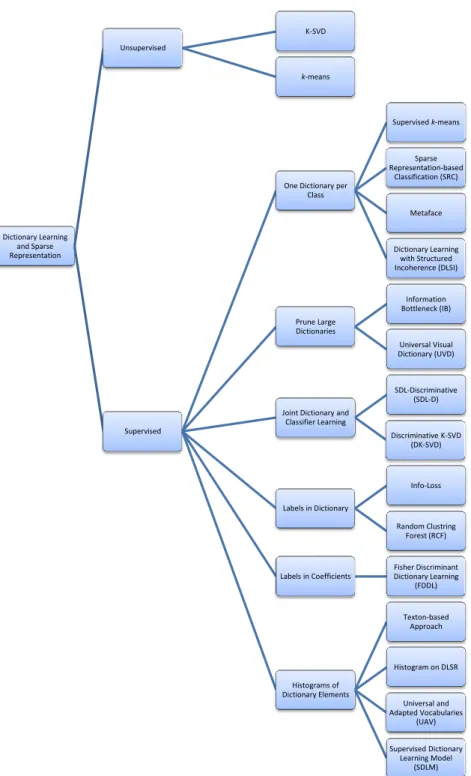
Figure 2.2 summarizes the taxonomy of dictionary learning and sparse representation techniques as presented in this chapter for quick reference.
In the next chapter, the mathematical formulation for the proposed approach will be explained, which I believe belongs to the fourth category of SDLs explained above, i.e., including category information to learn a supervised dictionary.
Dictionary Learning and Sparse Representation Unsupervised K-SVD k-means Supervised
One Dictionary per Class Supervised k-means Sparse Representation-based Classification (SRC) Metaface Dictionary Learning with Structured Incoherence (DLSI) Prune Large Dictionaries Information Bottleneck (IB) Universal Visual Dictionary (UVD)
Joint Dictionary and Classifier Learning SDL-Discriminative (SDL-D) Discriminative K-SVD (DK-SVD) Labels in Dictionary Info-Loss Random Clustring Forest (RCF) Labels in Coefficients Fisher Discriminant Dictionary Learning (FDDL) Histograms of Dictionary Elements Texton-based Approach Histogram on DLSR Universal and Adapted Vocabularies (UAV) Supervised Dictionary Learning Model (SDLM)
Chapter 3
Proposed Supervised Dictionary
Learning
Given a finite set of data samples X ∈ Rp×n, where p is the dimensionality of the data
and n is the number of data samples, in this chapter, we address the problem of linear decomposition ofXover a learned dictionaryD ∈Rd×k, wherekis the number of dictionary
atoms, by minimizing a loss function. The loss function is defined as the reconstruction error and`1-norm is added as the regularization penalty. The goal is to make the dictionary
D sufficiently discriminative over the classes.
To address this problem, we incorporate the class labels associated with the data sam-ples into the learning of the dictionary to make it discriminative. To incorporate the class labels into dictionary learning, it is proposed to decompose signals using some learned bases that represent them in a space where the dependency between the signals and their corresponding class labels is maximized. To this end, a(n) (in)dependency test measure between two random variables is needed. Here, it is proposed to use the Hilbert-Schmidt independence criterion (HSIC) as the (in)dependency measure. In this chapter, we first describe HSIC, and then provide the formulation for the proposed supervised dictionary learning (SDL) approach. Subsequently, kernelized SDL is formulated to enable embed-ding kernels, incluembed-ding data-dependent ones, into the proposed SDL. This can significantly improve the discrimination power of the designed dictionary, which is essential in difficult
classification tasks, as will be shown in our experiments in Section5.6 later.
3.1
Hilbert Schmidt Independence Criterion
There are several techniques in the literature to measure the (in)dependence of ran-dom variables including mutual information [61] and the Kullback-Leibler (KL) diver-gence [62]. In addition to these measures, there has recently been great interest in measur-ing (in)dependency usmeasur-ing criteria based on functions in reproducmeasur-ing kernel Hilbert spaces (RKHSs). Bach and Jordan [63] were the first to accomplish this, by introducing ker-nel dependence functionals that significantly outperformed alternative approaches. Later, Grettonet al. [32] proposed another kernel-based approach called the Hilbert-Schmidt in-dependence criterion (HSIC) to measure the (in)in-dependence of two random variables X
and Y. Since its introduction, the HSIC has been used in many applications, including feature selection [64], independent component analysis [65], and sorting/matching [66].
One can derive HSIC as a measure of (in)dependence between two random variables X
andY using two different approaches: first by computing the Hilbert-Schmidt norm of the cross-covariance operators in RKHSs as shown in [32,33]; or second, by computing maxi-mum mean discrepancy (MMD) of two distributions mapped to a high dimensional space, i.e., computed in RKHSs [67,68]. I believe that this latter approach is more straightforward and hence, use it to describe HSIC.
Let Z :={(x1,y1,), ...,(xn,yn)} ⊆ X × Y be n independent observations drawn from
p := PX ×Y. To investigate whether X and Y are independent, one needs to determine whether distribution pfactorizes, i.e., whether p is the same asq :=PX ×PY.
The means of the distributions are defined as follows
µ[PX ×Y] := Exy[v((x, y), .)], (3.1)
µ[PX ×PY] := ExEy[v((x, y), .)], (3.2)
where Exy is the expectation over (x, y) ∼ PX ×Y and kernel v((x, y),(x0, y0)) is defined in RKHS over X × Y. By computing the mean of distributions p and q in RKHS, higher
order statistics than the first order are effectively taken into account by mapping these distributions to a high-dimensional feature space. Hence, one can use MMD(p, q) :=
kµ[PX ×Y]−µ[PX ×PY]k2 as a measure of (in)dependence of the random variables X and
Y. The higher the value of MMD, the closer the two distributions pand q and hence, the more dependent are random variables X and Y.
Now suppose that H and G are two RKHSs in X and Y, respectively. Hence, by the Riesz representation theorem, there are feature mappingsφ(x) :X → Randψ(y) :Y →R
such that k(x, x0) = hφ(x), φ(x0)iH and l(y, y0) = hψ(y), ψ(y0)iG. Moreover, suppose that
v((x, y),(x0, y0)) = k(x, x0)l(y, y0), i.e., the RKHS is a direct product ofH⊗G of the RKHSs onX and Y. Then MMD(p, q) can be written as
MMD2(p, q) = kExy[k(x, .)l(y, .)]
−Ex[k(x, .)]Ey[l(y, .)]k22
= ExyEx0y0[k(x, x0)l(y, y0)]
−2ExEyEx0y0[k(x, x0)l(y, y0)]
+ExEyEx0Ey0[k(x, x0)l(y, y0)]. (3.3)
This is exactly the HSIC, and equivalent to the Hilbert-Schmidt norm of the cross-covariance operator in RKHSs [32].
For practical purposes, HSIC has to be estimated using a finite number of data samples. Considering Z :={(x1,y1,), ...,(xn,yn)} ⊆ X × Y as n independent observations drawn
fromp:=PX ×Y, an empirical estimate of HSIC is defined as follows [32]
HSIC(Z) = 1
(n−1)2tr(KHLH), (3.4)
where tr is the trace operator, H,K,L ∈ Rn×n, K
i,j = k(xi, xj), Li,j = l(yi, yj), and H =
I−n−1ee> (I is the identity matrix, and e is a vector of n ones, and hence, H is the centering matrix [69]). It is important to notice that according to (3.4), to maximize the dependency between two random variables X and Y, the empirical estimate of HSIC, i.e., tr(KHLH) should be maximized.
3.2
Supervised Dictionary Learning Formulation
To formulate the proposed SDL, one can start from the reconstruction error given in (2.3). Let there be a finite training set ofn data points, each of which consists of pfeatures, i.e., X = [x1,x2, ...,xn] ∈ Rp×n. Also suppose that features in data samples are centered, i.e.,
their mean is removed and hence, each row of X sums to zero. The problem statement is to find a linear decomposition of data X∈Rp×nusing some bases U∈
Rp×k such that the reconstruction error is minimum in the mean-squared sense, i.e.,
min U,Vi n X i=1 kxi−Uvik 2 2, (3.5)
where vi is the vector of k reconstruction coefficients. Equation (3.5) can be rewritten in
matrix form as follows
min
U,VkX−UVk
2
F, (3.6)
whereV ∈Rk×nis the matrix of coefficients. Since bothUand Vare unknown, this
prob-lem is ill-posed and does not have a unique solution unless some constraints are imposed on the bases U. If one, for example, assumes that the columns ofUare orthonormal, i.e., U>U=I, (3.6) can be written as a constrained optimization problem as follows
min U,V kX−UVk 2 F. s.t. U>U=I (3.7)
To further investigate the optimization problem in (3.7), one can assume that the matrix Uis fixed, and find the optimum matrix of coefficients V in terms ofX and Uby taking the derivative of the objective function given in (3.7) in respect to V
∂ ∂VkX−UVk 2 F = ∂ ∂Vtr[(X−UV) > (X−UV)] = ∂ ∂V[tr(X > X)−2tr(X>UV) + tr(V>U>UV)] > >
Equating the above derivative to zero and knowing that U>U=I, one obtains
V =U>X. (3.8)
By plugging the V found in (3.8) into the objective function of (3.7) we obtain
min U X−UU>X 2 F = minU tr[(X−UU > X)>(X−UU>X)] = min U [tr(X >X)−2tr(X>UU>X) + tr(X>UU>UU>X)] = max U tr(X > UU>X) = max U tr((U > X)>U>X).
LetK = (U>X)>U>X, which is a linear kernel on the transformed data in the subspace U>X; recalling that the features are centered in the original space, multiplying the data X by the centering matrix H does not have any effect. Hence, one can write
max U tr((U >X)>U>X) = max U tr((U >XH)>U>XHI) = max U tr(H(U > X)>U>XHI) = max U tr([(U > X)>U>X]HIH) = max U tr(KHIH), (3.9)
where I is the identity matrix. To derive (3.9), the identities H> = H and XH = XHI are used and it is also noted that the trace operator is invariant to the rotation of its arguments.
To enable providing an interpretation for (3.9), we recall that identity matrix I repre-sents a kernel on a random variable, where each data sample has maximum similarity to itself and no similarity, whatsoever, to others. Hence, based on empirical HSIC, the ob-jective function given in (3.9) indicates that the transformation Utransforms the centered data1 XH to a space where the dependency of random variables x and another random
variable whose kernel is identity matrix I is maximized. This means that using transfor-mationU, the random variablexis transformed such that each data sample has maximum similarity/correlation to itself and no similarity to other data samples. It is well known in the literature that these bases are the principal components of the signalX that represent the data in an uncorrelated space. With a few manipulations, the objective function given in (3.9) can be rewritten as follows:
max U tr((U > X)>U>X) = max U tr((U > XH)>U>XHI) = max U tr(HX > UU>XHI) = max U tr(U > XHIHX>U).
In other words, it is shown that the optimization problem in (3.7) is equivalent to max U tr(U > XHIHX>U), s.t. U>U=I (3.10) According to the Rayleigh-Ritz Theorem [70], the solution of the optimization problem in (3.10) is the top eigenvectors ofΦ=XHIHX>corresponding to the largest eigenvalues ofΦ. Here, XHIHX> is the covariance matrix of X.
To summarize, it was shown above that the linear decomposition of signals that min-imizes the reconstruction error in the mean-squared sense, represents the data in an un-correlated space. This is, in fact, the same as in the principal component analysis (PCA), where the top eigenvectors of the covariance matrix are computed. However, as mentioned before, although minimization of reconstruction error is the ultimate goal in applications such as denoising and coding, in classification tasks, the main goal is maximum discrimi-nation of classes. Hence, one is looking for a decomposition that represents the data in a space where the decomposed data have maximum dependency with their labels. To this end, we propose the new optimization problem as follows
max U tr(U > XHLHX>U), s.t. U>U=I (3.11)
Algorithm 1 Supervised Dictionary Learning
Input: Training data,Xtr, test data,Xts, kernel matrix of labels L, training data size, n,
size of dictionary, k.
Output: Dictionary, D, coefficients for training and test data, αtr and αts.
1: H←I−n−1ee>
2: Φ←XtrHLHX>tr
3: Compute Dictionary: D← eigenvectors of Φ corresponding to topk eigenvalues
4: Compute Training Coefficients: ReplaceXwith Xtr in (2.3), use (2.3) to compute
αtr given D
5: Compute Test Coefficients: Replace Xwith Xts in (2.3), use (2.3) to compute αts
given D
there is exactly one nonzero element in each columnY, where the position of the nonzero element indicates the class of the corresponding data sample. Similar to the previous case, the solution for the optimization problem given in (3.11) is the top eigenvectors of Φ = XHLHX>. These eigenvectors compose the supervised dictionary to be learned. This dictionary spans the space where the dependency between dataXand corresponding labelsY is maximized. The coefficients can be computed in this space using the lasso as given in (2.3). The optimization problem given in (3.11) compromises the reconstruction error to achieve a better discrimination power. In conclusion, the proposed supervised dictionary learning is given in Algorithm 1.
One important advantage of the proposed approach in Algorithm1is that the dictionary can be computed in closed form. Besides, learning the dictionary and the coefficients are performed separately, and it is not needed to learn these two iteratively and alternately, as is common in most supervised dictionary learning approaches in the literature (refer to Section2.2).
3.3
Proposed Kernelized SDL
One of the main advantages of the proposed formulation for SDL, compared to other techniques in the literature, is that one can easily embed a kernel into the formulation. This enables nonlinear transformation of the data into a high-dimensional feature space where the discrimination of classes can be more efficiently performed. This is especially beneficial when incorporating data-dependent kernels2, such as those based on normalized compression distance [34].
Kernelizing the proposed approach is straightforward. Suppose thatΨis a feature map representing the data in feature spaces H as follows:
Ψ:X → H
X7→Ψ(X). (3.12)
To kernelize the proposed SDL, it is sufficient to express the matrix of bases U as a linear combination of the projected data points into the feature space using representation theory [71], i.e., U=Ψ(X)W. In other words,W∈Rn×k representsU∈
Rp
0×k
in feature space Ψ(X)∈Rp0×n. Replacing X byΨ(X) andU byΨ(X)W in the objective function
of (3.11), one obtains
tr(U>Ψ(X)HLHΨ(X)>U) = tr(W>Ψ(X)>Ψ(X) HLHΨ(X)>Ψ(X)W) = tr(W>KHLHKW),
with the constraint
U>U = W>Ψ(X)>Ψ(X)W = W>KW,
whereK =Ψ(X)>Ψ(X) is a kernel function on data. Combining t
![Figure 2.1: The illustration of two steps of a texton-based system: (a) the generation of texton dictionary using supervised k -means (b) and the generation of features by computing the texton histograms on an image (from [25]).](https://thumb-us.123doks.com/thumbv2/123dok_us/778558.2598462/38.918.145.796.203.662/illustration-generation-dictionary-supervised-generation-features-computing-histograms.webp)


![Table 4.3: Classification error on test set for digit recognition on USPS data using proposed SDL compared with the most effective SDL approach reported in the literature on the same data [53]](https://thumb-us.123doks.com/thumbv2/123dok_us/778558.2598462/62.918.282.648.277.414/classification-recognition-proposed-compared-effective-approach-reported-literature.webp)