For Review Only
Projection based ensemble learning
for ordinal regression
M. P´erez-Ortiz, P.A. Guti´errez,Member, IEEE, and C. Herv´as-Mart´ınez, Member, IEEE,
Abstract—The classification of patterns into naturally ordered labels is referred to as ordinal regression. This paper proposes an ensemble methodology specifically adapted to this type of problems, which is based on computing different classification tasks through the formulation of different order hypotheses. Every single model is trained in order to distinguish between one given class (k) and all the remaining ones, but grouping
them in those classes with a rank lower than k, and those
with a rank higher than k. Therefore, it can be considered as
a reformulation of the well-known one-versus-all scheme. The base algorithm for the ensemble could be any threshold (or even probabilistic) method, such as the ones selected in this paper: kernel discriminant analysis, support vector machines and logistic regression (all reformulated to deal with ordinal regression problems). The method is seen to be competitive when compared with other state-of-the-art methodologies (both ordinal and nominal), by using six measures and a total offifteen ordinal datasets.Furthermore, an additional set of experiments is used to study the potential scalability and interpretability of the proposed method when using logistic regression as base methodology for the ensemble.
Index Terms—Ordinal regression, ensemble, discriminant anal-ysis, support vector machines, threshold models, relabelling
I. INTRODUCTION
O
RDINAL regression can be defined as a relatively new learning paradigm whose aim is to learn a prediction rule for ordered categories. This problem,firstly arising in statistics [2], is spreading rapidly and receiving a lot of attention from the pattern recognition and machine learning communities [3], [4] because it presents a wide range of applications in areas where human evaluation plays an important role, for example: psychology, medicine, information retrieval, etc. The main difference compared to standard regression is in the target variable, which is composed of finite and discrete category labels, the distances between them being unknown. Concern-ing classification, the variable to predict is not numerical or nominal, but ordinal; thus these categories show an implicit and natural order. An explanatory example of order among categories could be the Likert scale, a well-known methodol-ogy used for questionnaires, where the categories correspond to the level of agreement or disagreement with a series of M. P´erez-Ortiz, P.A. Guti´errez and C. Herv´as-Mart´ınez are with the Department of Computer Science and Numerical Analysis, University of C´ordoba, Campus de Rabanales, Albert Einstein building, 14071 - C´ordoba, Spain, e-mail:{i82perom, pagutierrez, chervas}@uco.es.This paper is a very significant extension of [1] with much additional material, including a comprehensive review of some ordinal regression methodologies, a more detailed description of the proposal with some changes, and a wider experimental section, where the results for different benchmark datasets and measures were analyzed. Besides, SVMs and logistic regression techniques formulated for ordinal regression were also considered in this work, both for ensemble construction and for comparison.
given statements. The scheme of a typical five-granularity Likert scale could be: {Strongly disagree, Disagree, Neither agree or disagree, Agree, Strongly Agree}, where the natural order among categories can be appreciated. The major problem within this kind of classification is that misclassification errors should not be treated equally: misclassifying the Strongly disagree class as Strongly agree should be more penalized than misclassifying it as Disagree. Therefore, several issues must be taken into account in order to exploit the presence of this order among categories. Firstly, this implicit data structure should be learnt by the classifier in order to minimize ordinal classification errors and, secondly, several measures or metrics should be developed in order to do so, given that simply being accurate might not be enough for this kind of problems.
Several approaches to tackle ordinal regression have been proposed in the domain of machine learning over the years, since the first work dating back to 1980 [2]. The simplest idea is to transform these ordinal scales into numeric values and solve the problem as a standard regression one. Kramer et al. investigated and proposed the use of a regression tree learner in this sense [5]. However, as outlined before, there is an important problem within these approaches: the fact that, in general, there is no knowledge about the distances between different classes. On the other hand, other works focused on addressing the problem by simply performing multinomial classification tasks (totally forgetting the order information) or by considering cost-sensitive classification [6] based on trivially imposed cost matrices. Some researchers approach the problem by decomposing the original ordinal regression task into a set of binary classification tasks [3], [7], or by formulating the original problem as one of extended binary classification [8], [9]. However, the most popular approach is clearly the use of threshold models [4], [10]–[12]. These methods are based on the idea that, in order to model ordinal classification problems from a regression perspective, one can assume that some underlying real-valued outcomes exist (also known as latent variable), although they are unobservable. Consequently, these methodologies estimate:
• A function f(x)that tries to predict the nature of those
underlying real-valued outcomes.
• A set of bias terms or thresholds b =
(b1, b2, . . . , bK−1)∈RK−1 (where K is the number of
classes in the problem) to represent the intervals in the range of f(x), whereb1≤b2≤. . .≤bK−1.
Nowadays, the ensemble paradigm is one of the most actively researched in pattern recognition and machine learn-ing [13]. This methodology imitates human nature to seek several opinions before making a crucial decision [14] and was
For Review Only
proposed as an alternative to the conventional “standalone”methods, which can be suboptimal. The main aspects ad-dressed in ensemble literature are: development of methods for reducing the dependence between classifiers, i.e. maximizing diversity, and development of effective combination rules.
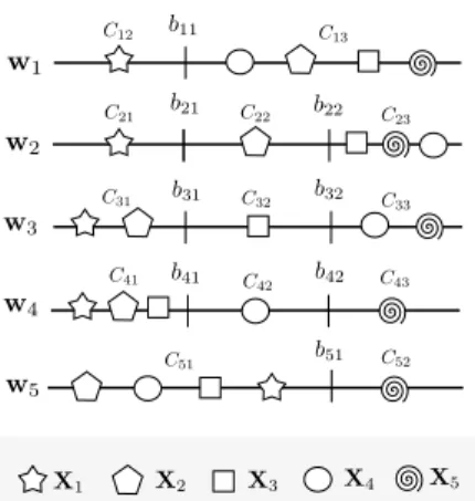
This paper contributes a novel and natural ensemble methodology to tackle ordinal information which could be used with any threshold model as base classifier. More specif-ically, in this paper kernel discriminant analysis (KDA) [4], [15] and support vector machines (SVM) [16], [17] were used for a first set of experiments, since these can be considered accurate and successful methods when adapted to ordinal regression [18], [19]. Moreover, logistic regression (LR) [2], [20] was considered for a set of large-scale datasets. The main motivation is the development of an ordinal ensemble algorithm which could benefit from the order information of the data to improve the performance of other existing techniques. As many classifiers as the number of classes are trained, and each single model is computed to differentiate each class from the remaining ones taking ordinal ranks into account, i.e. separating each class from the previous and following classes. The ensemble methodology proposed is based on decomposing ordinal regression problems into simpler classification tasks, where the order information is explicitly included. For aKclass ordinal regression problems, 2binary classification problems andK−2ordinal ones (each composed of three classes) are derived, in such a way that the main classification problem is simplified. This procedure can be appreciated in Fig. 1 for a 5 classes example. The main hypothesis is that the performance of any ordinal algorithm could be improved by simplifying classification tasks and formulating multiple order hypotheses which will be combined in a final decision function. The proposal can be seen as a reformulation of the one-versus-all idea to tackle ordinal regression. A set of experiments is presented in this paper, which tests and validates this methodology and other nominal and ordinal ones, taking into account15datasets with different characteristics. The results suggest that the proposal reaches a competitive performance level and is able to extract better quality classifiers from the order information in the class labels.Finally, a different set of experiments over two large-scale datasets is conducted to analyze the potential scalability and interpretability of the proposed ensemble.
Some advantages and decisions related to the proposal are now discussed. First of all, the choice of threshold models as base classifiers is justified because of their inherent advantage to lend themselves to probabilistic outputs, as these conditional probabilities of class membership are useful for constructing a more robust ensemble methodology. The proposal can be applied to any threshold model (indeed to any algorithm leading to probabilistic outputs), since the main idea is to compute one model to differentiate each class from the rest by taking ordinal ranks into account, and then extracting final output probabilities from the outcomes of each model. In addition, threshold methods depend to a great extent on the bias or threshold computation, which may be a complex handicap when dealing with kernel methods because of their tendency to over-fit. Instead of using crisp values, this study
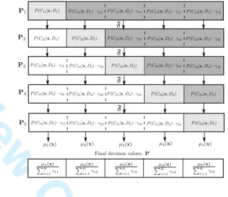
Fig. 1. Example showing different projections computed for the ensemble whenK = 5.Xi are the patterns associated to classi. The model trained
for separating classi-th from the remaining ones is denoted bywiand the
corresponding thresholds associated bybi1andbi2.Cijis used for denoting a synthetically constructed cluster of classes for decision makeri-th.
considers probability estimations to relax and alleviate the misclassification error of multiple order hypotheses. On the other hand, selecting the number of classifiers has always been one of the most important and controversial issues in the ensemble paradigm (this value is usually assigned to an odd number in order to avoid draws), but in this case it is very intuitive, as the number of classifiers would be preassigned to the number of classes in the sample. Also, inducing diversity in the classifiers is a crucial ingredient for developing robust ensemble techniques. However, in this case diversity is implicit in the technique, as each computed model will be composed of different data labelling and pattern distributions. Finally, the proposal could also be justified by the low number of ordinal ensemble methods existing in the literature.
The paper is organized as follows: Section II shows a de-scription of the methodologies used for the ensemble; Section III formally presents the proposal of this work; Section IV de-scribes the characteristics of the datasets and the experimental study; Section V analyzes the results obtained; and finally, Section VI outlines some conclusions and future work.
II. PREVIOUS NOTIONS
In this section, the terminology and notation that will be used throughout the entire work is established. The goal in classification is to assign an input vector x to one of
K discrete classes Ck, where k ∈ {1, . . . , K}. Thus, a formal framework for the ordinal regression problem could be introduced by considering an input space X∈Rd, where
d is the data dimensionality. To do so, an outcome space
Y ={C1,C2, . . . ,CK}is defined, where the labels are ordered due to the data ranking structure (C1≺C2≺· · ·≺CK, where
≺ denotes this order information). Let N be the number of patterns in the sample andNk the number of samples for the
k-th class. The objective in this kind of problem is to find a prediction function f : X → Y by using an i.i.d. sample
D={xi, yi}Ni=1∈X×Y.
The ensemble approach here proposed is applied to three well-known techniques: KDA, SVM and LR.Since they have
For Review Only
been reformulated to deal with ordinal regression problems abrief explanation of these methods is included in this section. A. Kernel discriminant learning
This learning paradigm (KDA) is one of the pioneer and leading techniques in the machine learning area, since it dates back to 1936 and has been widely used as much for supervised dimensionality reduction as for classification [21]. KDA has also been adapted to ordinal classification [4] by imposing a constraint on the projection to be computed, so that it will preserve and take advantage of the ordinal information from different classes. The method is known as kernel discriminant learning for ordinal regression (KDO) [4].
B. Support vector machines
The SVM paradigm [16], [22] is considered the most common kernel learning method for statistical pattern recog-nition. This study considers two of the most commonly used approaches for solving multiclass problems with SVMs: the one-vs-all formulation and the one-vs-one formulation.
Some works in the SVM literature have been focused on the reformulation of this successful paradigm to tackle ordinal regression problems [17], [23], [24]. All these approaches share one common objective which is the definition ofK−1 discriminant hyperplanes represented by the vector w and the scalars bias b1 ≤ . . . ≤ bK−1 in order to properly
separate training data into ordered classes by modeling ranks as intervals on the real line.
The proposal of Herbrich [23] derived the well-known SVM methodology for ordinal regression by making use of an independent distribution model and inducing an ordering in the space X that incurs the smallest number of inversions on pairs (xi,xj) of objects, the probability of that incurred inversion being given by a risk function for each pair of ranks. The main disadvantage of this algorithm is that the problem is formulated as a quadratic function directly depending on the training number of patterns.
On the other hand, the work of Shashua and Levin [24] introduced two different approaches: the former tries to max-imize the margin between the closest neighboring classes by applying the “fixed margin” policy and the latter allows for different margins where the sum of margins is maximized. The principal disadvantage of their proposal is that ordinal inequalities on the thresholds, b1≤b2≤. . .≤bK−1, are not
included in the formulation and this omission may result in disordered thresholds at the solution.
A third proposal of SVMs for ordinal regression is presented in the work of Chu and Keerthi [17]. This study also shows two different implementations for the idea. Both approaches guarantee that the thresholds are properly ordered at the optimal solution. Thefirst one only takes into account adjacent ranks for the determination of the thresholds, whereas in the second one, the whole training sample considering all ranks is used for the determination of each threshold, and samples in all the categories are allowed to contribute errors for each hyperplane. This second approach is called support vector ordinal regression with implicit constraints (SVOI).
From another point of view, ordinal regression can be trans-formed into several binary classification problems; one binary classifier can be derived for each problem, and the output of all classifiers can be combined to obtain afinal decision. The strategy is based on simply checking if the rank of a pattern is greater than a given rankk,1≤k≤K−1, which is indeed a binary classification question which is answered by each classifier. This approach is closely related to that proposed in this paper and wasfirst presented in the work of Frank & Hall [3] with C4.5 classification trees as base classifiers. However, SVMs have performed very competitively for binary problems, and a similar proposal was then considered for SVMs in the work of Waegeman & Boullart [7], but introducing specific weights into the different patterns. These weights try to reflect the fact that not all patterns in the “greater thank” class (for the binary classifier k) are equally far from k in the ordinal scale, and they should be treated differently when constructing the classifier (even though they belong to the same class). Both methods will be considered in the experimental section.
C. Logistic regression
In machine learning, LR [20] is a well-known methodology based on a regression analysis for classification problems. This method has been reformulated to deal with ordinal problems giving rise to the proportional odds model (POM) [2]. This model was the first threshold method applied to ordinal regression problems and it is based on a linear projection jointly trained with a set of thresholds by using a similar technique to that considered for nominal LR. Let h denote an arbitrary monotonic link function. The model:
h(P(y≤Cj|x)) =w�x−bj, j= 1, . . . , K−1, (1)
links the cumulative probabilities to a linear predictor and imposes an stochastic ordering of the spaceX, wherebjis the
threshold separatingCj andCj+1andwis a linear projection.
III. ENSEMBLE LEARNING FOR ORDINAL REGRESSION (ELOR)
In the previous section, three well-known classification methods have been presented: KDA, SVM and LR. These methods share one common and general objective which defines the optimization function: the maximization of the distance between different classes. Therefore, they depend greatly on the number of classes in the sample, hindering the separation between them when this number is high. Because of that, the proposed methodology tries to simplify the task of classification, and thus the optimization process. The proposal is intended to construct an ensemble which performs much simpler classification tasks. In order to do so, different decision models are computed, one for separating each class from the remaining ones (avoiding the problem of a great number of classes and aiming at a more balanced classification). The main motivation for this work could be found in the sentence of Albert Einstein, “Make everything as simple as possible, but not simpler”, because the original classification
For Review Only
task is simplified, but without forgetting the ordinal rankinginformation implicit in the data.
Various supervised and disjoint clusters (the term cluster is used to refer to a group of classes) are computed and classified taking into account the natural order of the classes, i.e. a label manipulation procedure is conducted in order to generate multiple hypotheses. In methods that manipulate the target attribute, instead of inducing a single complex classifier, several classifiers are induced with different and usually sim-pler representations of the target attribute [14]. One example of this is the one-versus-all methodology [25] (previously introduced for SVMs), where aK class classification problem is transformed into K binary classification ones. The one-vs-all paradigm seeks the i-th decision function fi(x), i ∈
{1, . . . , K}fulfilling thatfi(x)>0whenxbelongs to classi, andfi(x)<0whenxbelongs to one of the remaining classes. Therefore,fis used as a membership function for choosing the final prediction. The proposal described in this section can be seen as a one-versus-all reformulation for ordinal regression.
In ordinal regression, one-vs-all approach would not com-pute a fair classification, as the implicit order information would be ignored. For example, for a5-class problem,f4will try to distinguish between class4 and classes{1,2,3,5}. As class 5 is supposed to be closer to class 4 than to classes
{1,2,3}, it might be difficult to separate it from class4. The proposal tries to separate one class from the previous and the following ones, in such a way that the order among the classes is taken into account (see Fig. 1).
Furthermore, there exists another main issue apart from the exploitation of ordinal ranks by simplifying the classification task. It is well-known that the possible ways of combining the outputs of different classifiers in an ensemble depends on what information is obtained from individual members. When deal-ing with classification algorithms, the most common output for a learning procedure is the label predicted. However, in some cases, there is other information directly extractable from the classifier which may be helpful for improving classification performance, such as predicted probabilities. Threshold meth-ods present the problem of threshold computation which may often be a complex but important issue, asfinal classification entirely depends on those thresholds. In order to relax and alleviate this kind of errors, probability estimations are carried out by the proposed ensemble methodology.
Let us formally define the method. Given K different classes and corresponding events (C1,C2, . . . ,CK),Kdifferent classification problems will be computed by relabelling the data and training the learning algorithm with these relabelled patterns. By doing this,K different models will be obtained:
• Two of the models (thefirst one,i= 1, and the last one,
i = K) will compute binary classifications, separating classi from all the others. Standard KDA, SVM or LR will be applied in these cases.
• The rest of them (i ∈ {2, . . . , K−1}) will be three class classifiers, separating the corresponding class i-th from previous ones (1, . . . , i−1) and subsequent ones (i+ 1, . . . , K). Any of the previously presented ordinal algorithms could be used in order to maintain the ordinal rank of the classes (in these cases, the KDO, SVOI and
POM algorithms will be used).
An ensemble setDwill be defined consisting of a combination of K different decision makers, D = {D1, . . . , DK}. Each projection will be determined by the set of data to discriminate, as can be seen in Fig. 1 for K = 5, where Xi is the set of patterns belonging to classi-th.
The training set is defined as G = {G1, . . . ,GK}
for each member of the ensemble, where Gi =
{X(j|j<i), X(j|j=i), X(j|j>i)}. Note that, in the first and last
cases, one of the sets to discriminate will be the empty set, as there are no lower and higher ranking classes, respectively. Consequently, the cardinality of Gi will be |Gi| = 3, for
i∈{2, . . . , K−1}, and|Gi|= 2fori= 1andi=K. Clusters grouping different classes will be defined for each decision maker Di: Cij, 1 ≤ i ≤ K. The set of events to classify is defined in the following way:{Ci1 = (C1∪. . .∪
Ci−1),Ci2=Ci,Ci3= (Ci+1∪. . .∪CK)}, taking into account
that, in thefirst and the last classification tasks, some of them will be the empty set. These clusters result in different class targets (according to their rank): S1={1,2},Si={1,2,3}, (1< i < K), andSK={1,2}.
Then, each decision maker (Di) is determined by the set to discriminate (Gi), the labels Si, the computed optimal model (which in this case will be the optimal projection or hyperplane wi) and the set of thresholds for separating the classes (bi). Note that the number of thresholds for the classification corresponds to|Si|−1.
Although KDA, SVM and LR have been selected as base methods since they can be easily transformed to predict probabilities, the ensemble could be used with any threshold or probabilistic method. As when using threshold models it is possible to estimateK sets of probability, thefirst hypoth-esis is that the true values of P(Ci|x,D), i.e. the posterior probability, are the ones most agreed upon by the ensemble.
Although many types of uncertainty exist, probabilistic modelsfits surprisingly well in most pattern recognition prob-lems [13]. Because of that, this paper tries to construct a classifier by only taking estimated probabilistic information into account. For each pattern and decision maker i, the probability of belonging to class i will be calculated, along with the probability of belonging to the previous classes and the probability of belonging to the following ones. Then, a methodology for joining all the probabilities is proposed. For that, there are several issues to be addressed:
1) Distributing the probabilities within the cluster: when the specific model for separating classi-th from the rest is computed, three (or two) different supervised clusters are formed, one for the classes whose class target is less than i, one for class i and one for the classes whose class target is greater than i. These projections can be used to approximate the probability of belonging to a specific cluster (by using equations (2) and (3) of the next subsection), where one or more classes are represented. This probability has to be distributed among the different classes included in the cluster to obtain a
K-class probability distribution for each decision maker. 2) Combining the probabilities: as in any ensemble, a way has to be selected to combine the decisions of all
For Review Only
classifiers (average, product, majority voting, etc).3) Weighting more prominent classes: after distributing the probabilities, there are classes that are more prominent (for example extreme classes, which appear isolated in two of the projections, see Fig. 1). If a weighting method is not applied, all the patterns will be more likely to be classified in these classes.
A. Obtaining probability outputs
An important advantage of threshold methods [4], [10] over other algorithms is that their outputs can be easily transformed into conditional probabilities by analysing projected patterns and the corresponding thresholds. This is due to the fact that, in high-dimensional feature space, the histogram of each class projected by the discriminant function can be closely approximated by a given distribution. For example, given a pattern x and a decision maker Di the probability that this pattern has of belonging to clusterCij can be estimated using:
• The probit function, which computes a normal cumulative
distribution: P(Cij|x, Di) = 1 σ√2π � x −∞ e−(t2−σ2µ)2dt, (2)
• or the logit function, which computes the standard logistic sigmoid: P(Cij|x, Di) = 1 1 +e−t, (3) where i ∈ {1, . . . , K}, j = 1 or j ∈ {1,2}, t = wT
ix − bij is the projected pattern, wTi is the i-th transposed projection vector,bijis the corresponding bias for clusterj, and the assumption of µ = 0 and σ = 1
is made. Conditional probabilities can be useful, for instance, in applications where the output of a classifier needs to be combined with other information, and it is not only the class assignment that is interesting, but also its probability. Additionally, these probabilities allow us to combine the outputs ofK classifiers.
In this work, the probit function has been used for estimat-ing the probabilities in the case of the KDA methodologies, since these methods assume an unimodal normal distribution on the data. For LR methods, the logit function was used.On the other hand, as there is no guideline about which method should be used with nonparametric methods, such as SVMs, the logit function has been considered, which has been proved to show good results with this technique [26], [27].
B. Distributing the probabilities within the cluster
If the probability that a pattern belongs to a specific cluster is determined by a decision makerDi, then when the cluster
Cijhas only one class, the probability is directly defined but, if there are multiple classes, this probability should be distributed among the classes included in it (as can be seen in Fig. 2). One first idea could be simply to ignore all the clusters with more than one class and make use of the independent mem-bership values of the i-th single class of each decision maker (after applying the transformations proposed in the previous
subsection), in such a way that a vector of decision val-ues V = {P(C1|x, D1), P(C2|x, D2), . . . , P(CK|x, DK)} =
{P(C11|x, D1), P(C22|x, D2), . . . , P(CK2|x, DK)} is
com-puted and thefinal prediction would be the index of the max-imum value of it. Throughout this work, this methodology is referred to as simple ensemble learning for ordinal regression (SELOR) and has a significant disadvantage: the whole set of probabilities is not being considered.
More complex responses can be obtained if clusters with multiple classes are considered and the corresponding proba-bility is distributed among these classes. One possible way of distributing these probabilities is the following:
P(Ck|x, Di) =P(Cij|x, Di)·γik, ∀(Ck∈Cij), (4) withk∈{1, . . . , K},j∈{1,2,3} orj={1,2}, and taking into account thatγik= 1when|Cij|= 1.
Fig. 2. Example showing the different stages of the procedure. A combination functionFis used to combine the probability outputs and obtain allµk(x) values.
This γik weighting parameter could be chosen in many different ways:
1) Equally distributed probabilities: The probability of be-longing to class Ck for a specific decision maker Di (wherek∈{1, . . . , K}) is the probability of belonging to the clusterCij (taking into account that the patterns Xk associated toCk belongs to cluster Cij) divided by the number of different class targets involved in the cluster, in this case:
γik= 1
|Cij|
, ∀(Ck∈Cij).
For the sake of simplicity, this will be the method considered for all the experiments in this paper. 2) Distribution according to the number of patterns in each
class: The probability of belonging to class Ck for a decision makerDiwould be the probability of belonging to cluster Cij multiplied by the number of patterns in classCk with respect to the total involved in the cluster,
For Review Only
then: γik= �N n=1I(yn=Ck) �N n=1I(yn∈Cij) , ∀(Ck∈Cij), whereI(·)is defined as the indicator function.3) Distribution according to the inverse of the number of patterns of each class: The probability of belonging to class Ck for a decision maker Di would be, as before, the probability of belonging to clusterCij multiplied by the inverse of the number of patterns in class Ck with respect to the total involved in the cluster, thus:
γki= 1− �N n=1I(yn=Ck) �N n=1I(yn∈Cij) , ∀(Ck∈Cij). This alternative method could be considered for those unbalanced datasets where there is a special interest in classifying minority classes.
Note that the parameter γkiis calculated taking into account only training data.
C. Fusion of probabilities
After applying the method in the above subsection, a matrixP={P1, . . . ,PK}of probabilities is obtained, where Pi,j = pi,j = P(Cj|x, Di), satisfying that
�K
j=1pi,j = 1. Now, all the columns of this matrix are combined to obtain a final decision vector. A “nontrainable” combiner [13] is considered, i.e. no additional parameters will be tuned, so the ensemble will be ready for classification as soon as the base classifiers are trained. The membership for the j -th class is calculated using -the j-th column of the matrix:
µj(x) = F[p1,j(x), . . . , pK,j(x)], where F is defined as a combination function. The most commonly used choices for this function are the simple mean:
µj(x) = 1 K K � i=1 pi,j(x), (5)
and the product:
µj(x) = K
�
i=1
pi,j(x). (6)
A theoretical framework is offered for the average and product combiners in [28] based on the Kullback-Leibler divergence, which measures the distance between two proba-bility distributions. These combiners are the two most studied [29], but there is no guideline as to which one is better for a specific problem. In general, the average might be less accurate than the product for some problems, but it is more stable since a small change in a probability makes a bigger impact on the product than on the average.
D. Weighting more prominent classes
The distribution of probabilities considered in subsection III-B makes some classes receive more attention: for example, in Fig. 1, classes C1 andC5 appear isolated in the projections
more often than classesC2, C3 and C4, their computed
prob-ability being higher (a priori) than that of the other classes. Therefore, a weighting method is used in such a way that:
P�(Ci|x,D) = P(Ci|x,D) �K j=1γij . (7) E. Further considerations
In order to clarify all the concepts in previous subsections, a summary of the approach in this work is given in Fig. 3.
Pseudocode for the ordinal ensemble proposed
• Input: training inputs (xTr), training targets (tTr), test
inputs (xTs).
• Output: test predicted targets (tTs).
for i= 1to K
1. Compute the clustersGi fromxTr andtTr,
whereGi={X(j|j<i), X(j|j=i), X(j|j>i)}.
2. Train decision makerDi forGi:
optimal projectionwi and thresholds (bi) using either the binary or ordinal algorithm. 3. Project test data.
4. Compute test probabilities of belonging to each cluster.
5. Distribute clustered test probabilities among the classes for obtainingP, equation (4).
end for
Apply the defined Ffunction to the matrixP, equations (5) or (6).
Weight each column of Pby usingγij values (P�), equation (7).
Assign tTs choosing the index of maximum
value of each column in the decision vectorP�. Fig. 3. Different steps of the ensemble algorithm.
Concerning time complexity, the proposed ensemble will be obviously more time consuming than the base classifier, since it will compute K different models instead of one. However, the models computed will be simpler than the original ones, as the classification problem joins neighbor classes.
IV. EXPERIMENTS
Several benchmark datasets with different characteristics have been tested in order to validate the methodology pro-posed. Table I shows the characteristics of these datasets, where the number of patterns, attributes, classes and the class distribution (number of patterns per class) can be seen. These publicly available real ordinal classification datasets were extracted from benchmark repositories (UCI [30] and mldata.org [31], [32]). Also, some of the ordinal regression benchmark datasets (pyrim, machine, housing and abalone) provided by Chu et. al [12] were considered since they are widely used in the ordinal regression literature [4], [17]. These datasets do not originally represent ordinal classification tasks but regression ones. To turn regression into ordinal classification, the target variable is discretized intoKdifferent bins (representing classes, in this case K was assigned to5
For Review Only
TABLE ICHARACTERISTICS OF THE BENCHMARK DATASETS,ORDERED BY THE NUMBER OF CLASSES
Dataset #Pat. #Attr. #Classes Class distribution squash-stored (SS) 52 51 3 (23,21,8) squash-unstored (SU) 52 52 3 (24,24,4) tae (TA) 151 54 3 (49,50,52) newthyroid (NT) 215 5 3 (30,150,35) car (CA) 1728 21 4 (1210,384,69,65) eucalyptus (EU) 736 91 5 (180,107,130,214,105) pyrimx5 (P5) 74 27 5 (15,15,15,15,14) machinex5 (M5) 209 7 5 (42,42,42,42,41) housingx5 (H5) 506 14 5 (101,101,101,101,101) abalonex5 (A5) 4177 11 5 (836,836,835,835,835) automobile (AU) 205 71 6 (3,22,67,54,32,27) pyrimx10 (P10) 74 27 10 (8,8,8,8,7,7,7,7,7,7) machinex10 (M10) 209 7 10 (21,21,21,21,21,21,21,21,21,20) housingx10 (H10) 506 14 10 (51,51,51,51,51,51,50,50,50,50) abalonex10 (A10) 4177 11 10 (418. . .418,418,418,418,417,418,417,418,417), . . .
and 10), with equal frequency, as proposed in the previously mentioned works [4], [12], [17].
A. Methods compared
For an extensive analysis, several methods are compared. The proposed methodologies are applied using both SVM and KDA (and their adaptation to ordinal regression) as base methods. From now on, the methodologies are named as:
• Ensemble learning for ordinal regression using product
combiner with SVM and KDA (EPS and EPK).
• Ensemble learning for ordinal regression using average
combiner with SVM and KDA (EAS and EAK).
• Simple ensemble learning for ordinal regression with SVM and KDA (SS and SK).
These results have been compared with other state-of-the-art ordinal and nominal methods, such as:
1) Ordinal methods:
• Kernel discriminant learning for ordinal regression (KDO) [4] and support vector ordinal regression with implicit constraints (SVOI) [17], methods used as base classifiers in the ensemble proposals.
• Ordinal class classifier using the C4.5 as base classifier
(OCC) [3] and ordinal class classifier with specific ordinal weights (OCCW) and SVM [7], both discussed in Section II-B since they are closely related to the proposal.
• Extreme learning machine for ordinal regression (EL-MOR) [33] because the Extreme Learning Machine paradigm has demonstrated good scalability and gener-alization performance with a faster learning speed when compared to SVM [34].
• The POM algorithm [2] introduced in Section II-C.
2) Nominal methods:
• SVM classifier with one-vs-one methodology (SVM1) [35], and one-vs-all formulation (SVMA) [35]. These are the two main approaches for dealing with multiclass problems when using binary classifiers. Both are closely related to the proposal and it seems necessary to verify if they yield similar performances.
• SVM classifier using a probabilistic reformulation of the all paradigm (SVMPA). In this case, the one-vs-all approach is reformulated to estimate probabilities, just like the proposal in this work. That is, after per-forming each binary classification, the probabilities for each hypothesis are calculated and later combined by using a combination function (the product, as it has been the one presenting the best results in this experimental section). The purpose of this comparison is to check if the possible improvement of the ELOR method compared to the standard 1VsAll approach is due to the probabilistic component of the proposal. Equally distributed probabil-ities are considered and a weighting probability method is not necessary, because all the classes receive the same attention.
• AdaBoostM1 using C4.5 as base classifier (AdaB.). This
ensemble classifier is one of the most widely used in the machine learning literature, given its proven performance. KDO and the proposed ensemble variants were implemented using Matlab, as well as the POM model available through the
mnrfit function. The authors of SVOI provide a publicly
available software1, which was considered both for the stan-dalone version and the proposed ensemble version. The
well-know libsvm implementation2 was considered for all the
different versions of the SVM ensembles and for OCCW. The Matlab code for ELM3 was adapted to implement ELMOR. Finally, the Weka4machine learning framework [36] provided the implementations for OCC and AdaB.
B. Evaluated measures
Several measures can be considered for evaluating ordinal classifiers. The most common ones in machine learning are the mean absolute error (M AE) and the mean zero-one error (M ZE) [4], [17], [18], being M ZE = 1 − Acc, where
Acc is the accuracy or correct classification rate. However, as previously said, these measures are not the best option, for example, when measuring performance in the presence of class imbalances [37] and/or when the costs of different errors vary markedly. Because of that, this work makes use of different kind of measures to evaluate classifier performance.
The mean absolute error (M AE) is the average deviation in absolute value of the predicted class from the true class [37]:
M AE= 1
N
�N
i=1e(xi),wheree(xi) =|r(yi)−r(y∗i)|is the distance between the true and the predicted ranks (r(y)being the rank for a given targety), and, then, M AE values range from 0 to K−1 (maximum deviation in number of ranks between two labels).
The average mean absolute error (AM AE) is the mean of theM AE across classes [37]:AM AE= K1 �K
k=1M AEk= 1 K �K k=1N1k �Nk
i=1e(xi),whereAM AE values range from 0
to K−1.
The maximum mean absolute error (M M AE) for all the classes is the M AEvalue considering only the patterns from
1http://www.gatsby.ucl.ac.uk/∼chuwei/svor.htm
2http://www.csie.ntu.edu.tw/∼cjlin/libsvm/
3http://www.ntu.edu.sg/home/egbhuang/ 4http://www.cs.waikato.ac.nz/ml/weka/
For Review Only
the class with the greatest distance between true labels andpredicted ones: M M AE = max{M AEk;k∈{1, . . . , K}},
whereM AEkis theM AEvalue considering only the patterns from the k-th class and Nk is the number of pattern in this class. M M AE values range from 0 to K − 1. This measure was recently proposed [38] and its advantage is that a low M M AE represents a low error for all independently considered classes.
The Kendall’s τb is a statistic used to measure the as-sociation between two measured quantities. Specifically, it is a measure of rank correlation: τb =
�c∗ ijcij √�c∗2 ij �c2 ij , i ∈ {1, . . . , N}, j∈{1, . . . , N},wherec∗ ij is+1ify∗i is greater than (in the ordinal scale)y∗
j,0ifyi∗andy∗j are the same, and
−1ify∗
i is lower thanyj∗, and the same forcij.τbvalues range from−1(maximum disagreement between prediction and true label), to0(no correlation between them) and to1(maximum agreement). One important advantage of this correlation index is that it makes no assumption about the scale of the ranks.
The weighted Kappa (Wk) is a modified version of the Kappa statistic to allow different weights to differ-ent levels of aggregation between two variables: Wk =
po(w)−pe(w) 1−pe(w) ,withpo(w)= 1 n �K i=1 �K j=1wijnij,andpe(w)= 1 n2 �K i=1 �K
j=1wijni·n·j, where nij is the number of times the patterns are predicted by the classifier to be in classjwhen they really are in classi,ni·=�jK=1nij andn·j=
�K
i=1nij fori, j ∈{1, . . . , K}. The weightwij =|i−j|quantifies the degree of discrepancy between true (yi) and predicted (y∗
j) categories, and Wk range from−1to1.
In this sense, different character measures are used. Firstly, theAccmeasure, the most common for classification, reports, in terms of a ratio, how well the classifier works without making any distinction between the classes in the problem. Secondly, the standard M AE measure, well-known for ordi-nal regression problems, considers different misclassification errors. Also, two novel measures are used in order to prove whether the proposal achieves more balanced predictions when the number of patterns is very different for each class. The
AM AE metric reports how well all the classes are classified and theM M AE gives information about the worst classified class. Finally, two different statistics are considered, in order to measure the association between prediction and true labelling. C. Evaluation and model selection
Regarding the experimental setup, a holdout stratified tech-nique was applied to divide the datasets30times, using75% of the patterns for training and the remaining25%for testing. For the regression datasets provided by Chu et. al [12] (pyrim, machine, housing and abalone), the number of random splits was 20and the number of training and test patterns are the same as those presented in the corresponding works [12], [17]. The partitions were the same for all methods compared and one model was obtained and evaluated (in the test set), for each split. Finally, the results are taken as the mean and standard deviation of the measures over the 30test sets.
The parameters of each algorithm are chosen using a nested validation with each of the training sets (k-fold method with
k= 5) and the cross-validation criteria is theM AE since it
can be considered the most common one in ordinal regression. The kernel selected for all the algorithms is the Gaussian one,
K(x,y) = exp�−�x−σ2y�2
�
whereσis the standard deviation.
For every tested kernel method (KDA and SVM meth-ods), the kernel width was selected within these values
{10−3,10−2, . . . ,103}, as the cost parameter associated with
SVM methods. The parameter u for avoiding singular-ity (for the methods based on KDA) was selected within
{10−4,10−3,10−2,10−1}, and theC parameter for the KDO
was selected within the following ones {10−1,100,101}.
D. Results
This section presents three different types of experiments. Firstly, a synthetic dataset is designed in order to show the advantages of the proposal graphically when comparing it with the one-vs-all standard formulation. Secondly, the results ob-tained are compared for the 15datasets previously presented, with the6ensemble methodologies proposed and10 state-of-the-art algorithms, using a set of6different selected measures.
Finally, a different set of experiments with large-scale ordinal datasets is performed to analyze the potential scalability and interpretability of the proposed method.
−10 −5 0 5 10 15 20 25 30 −5 0 5 10 15 20 25 30
Fig. 4. Synthetic dataset and the optimal projection computed by linear discriminant analysis for ordinal regression [4].
1) Graphical representation of the proposal: In this sub-section, a new synthetic dataset has been designed in order to show the main differences and advantages when comparing the ordinal version of the algorithms and the one-vs-all standard proposal. The graphical representation of the dataset can be seen in Figures 4 and 5.
Figure 4 shows the ordinal projection computed and the projected patterns for the dataset. Linear discriminant analysis for ordinal regression has been used for this (without using the kernel trick) to allow the representation of the results, due to the fact that the kernel trick would classify the dataset structure perfectly. Taking into account the final projection, it can be observed that classes 2,3 and4 are not very well-classified since they present some overlapping on the projection.
On the other hand, Figure 5 shows various projections com-puted and the patterns projected by the proposed procedure and the one-vs-all paradigm (also using linear discriminant anal-ysis). The computed projections for the first and last classes
For Review Only
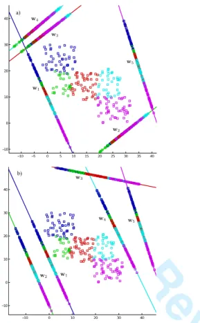
−10 −5 0 5 10 15 20 25 30 35 40 −10 0 10 20 30 40 −10 0 10 20 30 40 −10 0 10 20 30 40 a) b)Fig. 5. Graphical representation of the different projections computed for the synthetic dataset using linear discriminant analysis: a) Projections computed by the one-vs-all formulation. b) Projections computed by the ordinal ensemble methodology proposed.
are seen to be the same as in the previous case, since the classification tasks are the same. But in this case, the projection for the rest of the classes allows better separation since some order among the classes is supposed. For example,w3allows a
clearer separation for the classes than the computedw3in the
one-vs-all formulation, where the classes {1,2,3} are mixed in the projection. Each single class is seen to be well-classified in at least one model, and also the classes are ordered in the projection so that some information is implicit in the model.
2) Experimental results: The algorithms compared here have been run and optimized under the same conditions and using the same parameter cross-validation. First, the different ensemble proposals and their base algorithms are compared, and then the rest of the state-of-the-art methods are considered. Table II shows the mean ranking for the proposals and the base methodologies for all 15 datasets, taking into account 6 different measures, which may help the reader to evaluate the value of the proposal. This table only considers the mean ranking (over all the datasets) obtained for each method and each metric. In this case (where8algorithms were compared), a ranking of 1 is assigned to the best method for a given dataset, and a ranking of8to the one which provides the worst performance. In this table and all the following ones, the best method is in bold face and the second one in italics. The mean ranking considering all the metrics has also been included in the table as a summary. In almost all cases, the ensemble
TABLE II
MEAN RANKINGS OF THE15DATASETS CONSIDERED FOR THE ENSEMBLE METHODOLOGIES PROPOSED AND THE BASE ALGORITHMS USED.
Method
Measure KDO EPK EAK SK SVOI EPS EAS SS Acc 6.73 3.87 4.80 5.77 3.87 2.07 3.50 5.40 M AE 6.27 4.70 4.60 6.67 3.30 2.67 2.60 5.20 AM AE 6.27 4.70 4.37 6.27 3.00 2.53 3.33 5.53 M M AE 5.27 4.83 3.70 5.67 3.53 3.40 4.00 5.60 τb 5.47 3.97 4.57 7.00 3.27 2.87 3.07 5.80 Wk 5.73 3.57 5.23 6.87 3.47 2.00 3.60 5.53 Average 5.96 4.27 4.54 6.37 3.41 2.59 3.35 5.51
achieves better results than the initial algorithms. Specifically, it can be seen that the best results or the second best results for almost all the metrics tested are achieved by applying the EPS proposal. The complete tables of results showing the means and standard deviations for all benchmark datasets and metrics are not included in this work for the sake of simplicity and readability, but they can be found on a public webpage5.
To quantify whether a statistical difference exists among the algorithms compared in Table II, a procedure is employed to compare multiple classifiers in multiple datasets [39]. First of all, a Friedman’s non-parametric test with a significance level of α= 0.05has been carried out to determine the statistical
significance of the differences in the mean ranking results for each measure selected. The test rejected the null-hypothesis that all algorithms perform similarly when α = 0.05 for
all the selected metrics, stating then that the differences in mean rankings ofAcc,M AE,AM AE,M M AE, Kendall’s
τband Wk are statistically significant. Specifically, the confi -dence interval for this number of datasets and algorithms is
C0 = (0, F(α=0.05) = 2.10), and the corresponding F-value for each metric was 7.95 ∈/ C0, 9.30 ∈/ C0, 7.65 ∈/ C0, 2.47 ∈/ C0, 8.11 ∈/ C0 and 10.22 ∈/ C0 for Acc, M AE,
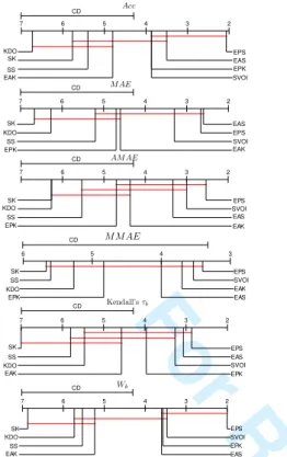
AM AE,M M AE, Kendall’sτb andWk, respectively. On the basis of this rejection, the Nemenyi post-hoc test is used to compare all classifiers to one another. This test considers that the performance of any two classifiers is deemed significantly different if their mean ranks differ by at least the critical difference (CD), which depends on the number of datasets and methods. 5% significance confidence was considered (α = 0.05) to obtain this CD and the results
can be observed in Figure 6, which shows CD diagrams as proposed in [39]. Each method is represented as a point on a ranking scale, corresponding to its mean ranking performance. CD segments are included to measure the separation needed between methods in order to assess statistical differences. Red lines group algorithms for which statistically significant, different mean ranking performance can not be assessed.
From the results of the statistical tests and from the tables, several conclusions can be drawn: firstly, one could notice by analysing mean rankings that the techniques based on SVMs present a clearly better performance than the ones based on KDA, and the ensemble procedure based on SVM usually outperforms the results obtained by the ensemble based on KDA, independently of the combiner or metric
For Review Only
7 6 5 4 3 2 CD SVOI SK 7 6 5 4 3 2 CD 7 6 5 4 3 2 CD EPS SVOI EAS EAK EPK SS KDO SK 6 5 4 3 CD EPS SVOI EAK EAS EPK KDO SS SK 7 6 5 4 3 2 CD EPS EAS SVOI EPK EAK KDO SS SK 7 6 5 4 3 2 CD EPS SVOI EPK EAS EAK SS KDO SK SS EAK EPS EAS EPK EPK EAS EPS KDO SK KDO SS SVOI EAKFig. 6. Results and ranking of the Nemenyi statistical test for proposals and base methods.
used. Secondly, no significant differences can be observed by analysing different probability combiners, although the great majority of the results show better performance using the product combiner. Also, the methodology SELOR (SK and SS) can not be considered to be a good approach since its performance is worse than that of the base algorithms in many cases. Thus, it has been shown that considering all the probability information, performance can be significantly improved. Last but not least, the ensemble procedure seems to be a good approach to tackle ordinal regression since it leads to an improvement in the results obtained by several algorithms of the state-of-the-art (as the base classifiers used: KDO and SVOI) taking different measures into account. This can be easily seen by analysing the Nemenyi post-hocfigures. To complete this section, a table similar to the previous one but containing the mean rankings for the rest of the state-of-the-art algorithms is shown in Table III. The EPS proposal is also included in this table, since, as stated before, it could be considered the proposal with the best performance. This table shows that the EPS procedure seems to be competitive for all measures (both ordinal and nominal), since it always obtains the best mean ranking. The second best method is OCCW, with the second position for all measures.
Table III shows that the EPS methodology is the best one in performance for all6metrics, improving the performances of4 different ordinal classifiers and4nominal ones, and achieving a considerable balance betweenAcc, ordinal measures, those appropriate for imbalanced datasets, and correlation ones.
In this case, the non-parametric Friedman’s test with a sig-nificance level ofα= 0.05was also applied to the mean
rank-TABLE III
MEAN RANKINGS OF THE15DATASETS FOR THE SELECTED ENSEMBLE METHODOLOGY AND OTHER STATE-OF-THE-ART METHODS.
Method
Measure EPS OCCW OCC ELMOR POM SVM1 SVMA SVMPA AdaB. Acc 2.03 2.60 6.67 5.20 6.23 3.50 5.40 7.43 5.93 M AE 1.63 3.07 6.10 4.67 5.93 4.57 6.00 7.30 5.73 AM AE 1.67 3.60 6.20 4.80 5.40 4.70 5.90 7.00 5.73 M M AE 1.67 4.00 6.27 4.27 4.93 5.27 6.13 7.00 5.47 τb 1.60 2.87 6.60 4.73 5.20 4.53 6.00 7.33 6.13 Wk 1.40 3.07 6.73 5.27 5.27 4.27 5.73 7.33 5.93 Average 1.67 3.20 6.43 4.82 5.49 4.47 5.86 7.23 5.82
ings for each measure. The test rejected the null-hypothesis that all algorithms perform similarly when α = 0.05 for all
the selected metrics, stating then that the differences in the mean ranking of Acc, M AE,AM AE, M M AE, Kendall’s
τband Wk are statistically significant. Specifically, the confi -dence interval for this number of datasets and algorithms is
C0 = (0, F(α=0.05) = 2.02), and the corresponding F-value for each metric was 12.33 ∈/ C0, 9.52 ∈/ C0, 7.08 ∈/ C0, 6.91 ∈/ C0, 11.24 ∈/ C0 and 11.63 ∈/ C0 for Acc, M AE,
AM AE,M M AE, Kendall’sτb andWk, respectively. It is well-known that the Nemenyi approach comparing all classifiers to one another in a post-hoc test is not as sensitive as the approach comparing all classifiers to a given classifier (known as a control method) [39]. The Holm test performs this latter type of comparison, only considering the comparison between the control method and all the alter-natives, and sequentially testing the hypotheses ranked by their significance. The ordered p-values will be denoted by
p1≤p2≤. . .≤pk−1, wherekis the number of comparisons
made. This step-down procedure comparespiwith a corrected version of the level of significance α/(k−1), starting with
the most significantp-value (p1). Ifpi is below the corrected
α, the null hypothesis is rejected and the next comparison is
performed. When a certain null hypothesis can not be rejected, all the remaining ones are also retained. The results of this test (correctedαvalues andp-values) for all the measures are
included in Table IV, where EPS is used as the control method. This table shows that the EPS presents statistically sig-nificant differences for α = 0.05 for almost all measures
with respect to almost all methods, except for SVM1 (when using Acc) and OCCW (when using some of the metrics). No statistically significant differences could be assessed when comparing EPS to SVM1 forAcc, which is, in fact, a nominal method not designed to deal with ordinal problems. Further-more, it can be seen that the proposal presents significant statistical differences for α = 0.05 and theM M AE metric
with respect to the OCCW methodology, which could be considered the procedure most similar to the one designed in this work, and that the differences forAM AE andWk are also significant forα = 0.10. In any case, it is important to
remember that the mean rankings are always the best for EPS. From these results, several conclusions can be drawn:firstly, as said before, it has been proven that an ordinal regression point of view is needed when dealing with some given order among categories, because, although a nominal algorithm may perform well when taking into account, for example, the
For Review Only
TABLE IVRESULTS OF THEHOLM PROCEDURE USINGEPSAS THE CONTROL METHOD WHEN COMPARED TO OTHER STATE-OF-THE-ART METHODS: CORRECTEDαVALUES,COMPARED METHOD ANDp-VALUES,ALL OF
THEM ORDERED BY THE NUMBER OF COMPARISON(i).
Acc M AE AM AE
i α∗0.05 α∗0.10 Method pi Method pi Method pi 1 0.0063 0.0125 SVMPA 0.0000• SVMPA 0.0000• SVMPA 0.0000•
2 0.0071 0.0143 OCC 0.0000• OCC 0.0000• OCC 0.0000•
3 0.0083 0.0167 POM 0.0000• SVMA 0.0000• SVMA 0.0000•
4 0.0100 0.0200 AdaB. 0.0001• POM 0.0000• AdaB. 0.0001•
5 0.0125 0.0250 SVMA 0.0008• AdaB. 0.0000• POM 0.0002•
6 0.0167 0.0333 ELMOR 0.0015• ELMOR 0.0024• ELMOR 0.0017•
7 0.0250 0.0500 SVM1 0.1425 SVM1 0.0034• SVM1 0.0024•
8 0.0500 0.1000 OCCW 0.5709 OCCW 0.1518 OCCW 0.0532◦
M M AE τb Wk
i α∗0.05 α∗0.10 Method pi Method pi Method pi 1 0.0063 0.0125 SVMPA 0.0000• SVMPA 0.0000• SVMPA 0.0000•
2 0.0071 0.0143 OCC 0.0000• OCC 0.0000• OCC 0.0000•
3 0.0083 0.0167 SVMA 0.0000• AdaB. 0.0000• AdaB. 0.0000•
4 0.0100 0.0200 AdaB. 0.0001• SVMA 0.0000• SVMA 0.0000•
5 0.0125 0.0250 SVM1 0.0003• POM 0.0003• POM 0.0001•
6 0.0167 0.0333 POM 0.0011• ELMOR 0.0017• ELMOR 0.0001•
7 0.0250 0.0500 ELMOR 0.0093• SVM1 0.0034• SVM1 0.0042•
8 0.0500 0.1000 OCCW 0.0196• OCCW 0.2053 OCCW 0.0956◦
•: Statistical difference withα= 0.05
◦: Statistical difference withα= 0.10
measure of accuracy, it may fail when taking into account other ordinal measures. Secondly, as statistically significant differences exist for all the metrics selected when taking into account the different one-vs-all proposals (the nominal proposal for reformulating the SVM paradigm and the pro-posal in this work), ELOR seems to present clear advantages over the one-vs-all nominal paradigm, when tackling ordinal classification. Finally, it can be concluded that the combination of single classifiers, aiming at a more accurate classification decision at the expense of increased complexity, seems to be a good idea in this case, since it improves the performance of other state-of-the-art methodologies significantly.
3) Large-scale datasets and interpretability: Once the per-formance of the proposed method has been extensively val-idated making statistical comparisons to other state-of-the-art methodologies for different measures and datasets, there are some unanswered issues such as the scalability of the algorithm or its possible interpretability, which is the main aim of this subsection. However, these issues are more related to the choice of the base algorithm for the ensemble because it will obviously determine if the algorithm could be used with large-scale datasets or for model interpretability purposes. The complexity of the kernel methods previously used as base methodologies for the ensemble depend directly on the number of training patterns [4] and their interpretability is difficult. Because of this reason, a simpler and more inter-pretable method is used for the following experiments. This method does not present parameters to optimize and it is also designed for ordinal regression. It is a linear model, leading generally to a lower performance (see Table III of this paper or other studies in the ordinal classification literature [18], [19]). However, it provides us with a probabilistic output, a simpler model and a better interpretability. The method used is the POM algorithm [2] which was used for comparison purposes in the previous experimental subsection. Moreover, standard binary LR is used for the binary decompositions.
This methodology, can be considered as interpretable in the sense that it could give us clues about the importance of each attribute for modelling the dependent variable.
For the experiments, two real ordinal datasets have been used. First, the Happiness dataset was extracted from the “European Social Survey”6 considering year 2010 and 26
countries. It represents the complex problem of predicting the individual happiness by using certain characteristics, beliefs and life circumstances in a Likert scale (examples of some input variables are: the health of the person, if he or she has anyone to discuss personal matters, whether he or she takes part in social activities, etc). We selected 13 attributes and considered 5 classes. The dataset was composed of 41472
instances (missing values were removed for simplicity). For more information of this dataset see the webpage associated to this paper5. Secondly, the SpanishFleet dataset was obtained from the “Fleet Register On the Net” considering year 2012 and the whole Spanish fleet to predict the commitment to sustainability of the Spanish vessels, using a categorization of the overexploitation of the gears employed provided by the Food and Agriculture Organization of the United Nations. This dataset was composed of10460instances, 6 attributes and 10 classes. For more information of this dataset see [40].
Concerning the experiments on these datasets, the same aforementioned experimental design was used (i.e.,30random repetitions of a stratified holdout, with 75% for training and 25% for the test set). To analyze the scalability of the algorithms, the complete time in seconds for executing each algorithm is also included in the results (note that the same machine architecture was used). The methods tested are: 1) the POM algorithm (which was previously presented) 2) ordinal class classifier using POM as base classifier (OCCP) and 3) ensemble learning for ordinal regression using product combiner and the POM algorithm as base classifier (EPP). We considered OCCP because it is a decomposition method which can be said to follow the same philosophy of EPP but using binary classifiers.
The results of these experiments can be seen in Table V. From these results, it can be seen that the proposed method outperforms in all the metrics the base classifier and, in most of the cases, the ordinal binary decomposition method (OCCP), thus providing more robust results. Furthermore, although both classification problems are complex because of the variable to predict, the obtained results are very promising (e.g., in
M AE and AM AE). With regard to the execution time, the computational complexity of the methodology is affordable, even for large-scale problems. Furthermore, as it can be seen in the experiments (comparing the time obtained in both datasets), the time complexity of the algorithm depends to a greater extent on the number of classes (because it determines the number of decompositions to perform) rather than on the number of samples.
Concerning interpretability, the decomposition proposed provides us with additional information in the sense that one model for differentiating each class from the previous and following classes is computed. Therefore, instead of being
For Review Only
TABLE VMEAN TEST VALUES FOR THE DIFFERENT METHODS CONSIDERED.
Happiness
Metrics POM OCCP EPP
Acc 60.78±0.15 63.44±0.26 63.73±0.25 M AE 0.449±0.002 0.402±0.003 0.397±0.003 AM AE 1.259±0.011 1.028±0.016 1.002±0.014 M M AE 2.580±0.051 1.953±0.081 1.950±0.075 τb 0.232±0.007 0.350±0.007 0.375±0.006 Wk 0.088±0.005 0.256±0.006 0.293±0.005 Time 23.41±4.34 32.49±0.50 49.00±0.47 SpanishFleet
Metrics POM OCC(POM) EPP
Acc 83.33±0.52 86.62±0.39 85.87±0.28 M AE 0.443±0.012 0.406±0.015 0.388±0.010 AM AE 2.104±0.048 2.200±0.117 1.943±0.062 M M AE 6.880±0.116 5.996±0.370 6.594±0.151 τb 0.611±0.013 0.602±0.021 0.631±0.017 Wk 0.620±0.012 0.665±0.013 0.678±0.008 Time 44.21±2.24 173.52±1.33 225.18±2.11
vided with a model for tackling the whole learning problem, we obtain a model for discriminating each class and we could analyze independently the variables most determining.
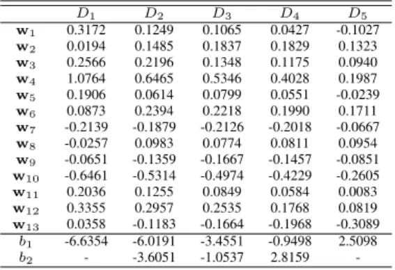
To better visualize the interpretability of the model, let us analyze an example with the Happiness dataset. The best model (in this case the one performing better in terms of
M AE for EPP) has been selected for the analysis. This model can be seen in Table VI. Note that both D1 and D5 are binary classifiers with a single threshold. The most important variables for modelling the labelling are the ones with higher
|wi| value, for example, it can be seen thatx4 (satisfaction
with present state of economy in country) presents a high impact on the variable to predict and so dox10(the subjective health of the person). One should note that although the sign of
wicould also be used for an interpretability analysis, it could
depend on the variable coding (in the case of the subjective health the variable is encoded from very good health to very bad health, thus this variable is negatively correlated with the label). Furthermore, it can be seen that variables important for different models are not so determining for others (analyze the case ofx1,x2orx13). Besides, as part of the model analysis,
it can be said that having someone to discuss personal matters (x7) makes you happier (note that the “yes” have been encoded
as 0 and “no” as 1).
As a final remark, if we order the variables taking into account their importance for each model (as said, the |wi|
value), it can be observed that some variables have almost no influence for discriminating certain classes (see Table VII). For example: being member of a group discriminated in your country or not (x11) is an influential variable for determining if you are extremely unhappy, but not for determining if you are extremely happy (it is at the last position). On the contrary, thinking that is important to help people and care for others well-being (x13) is indeed a determining variable
for the happiest (it is at thefirst position).
V. CONCLUSIONS AND FUTURE WORK
The methodology here proposed is based on the com-putation of different classification tasks, by performing a relabelling process which takes ordinal data information into
TABLE VI
BEST SET OF MODELSDi,1≤i≤5,OBTAINED BY THE PROPOSED ORDINAL ENSEMBLE USING THEPOMALGORITHM AS BASE METHOD.
THE MEANING OF EACH VARIABLE CAN BE FOUND IN THE WEBSITE ASSOCIATED TO THIS PAPER.
D1 D2 D3 D4 D5 w1 0.3172 0.1249 0.1065 0.0427 -0.1027 w2 0.0194 0.1485 0.1837 0.1829 0.1323 w3 0.2566 0.2196 0.1348 0.1175 0.0940 w4 1.0764 0.6465 0.5346 0.4028 0.1987 w5 0.1906 0.0614 0.0799 0.0551 -0.0239 w6 0.0873 0.2394 0.2218 0.1990 0.1711 w7 -0.2139 -0.1879 -0.2126 -0.2018 -0.0667 w8 -0.0257 0.0983 0.0774 0.0811 0.0954 w9 -0.0651 -0.1359 -0.1667 -0.1457 -0.0851 w10 -0.6461 -0.5314 -0.4974 -0.4229 -0.2605 w11 0.2036 0.1255 0.0849 0.0584 0.0083 w12 0.3355 0.2957 0.2535 0.1768 0.0819 w13 0.0358 -0.1183 -0.1664 -0.1968 -0.3089 b1 -6.6354 -6.0191 -3.4551 -0.9498 2.5098 b2 - -3.6051 -1.0537 2.8159 -TABLE VII
RANKING OF VARIABLES FOR THE DIFFERENT MODELS.
D1 D2 D3 D4 D5 x4 x4 x4 x10 x13 x10 x10 x10 x4 x10 x12 x12 x12 x7 x4 x1 x6 x6 x6 x6 x3 x3 x7 x13 x2 x7 x7 x2 x2 x1 x11 x2 x9 x12 x8 x5 x9 x13 x9 x3 x6 x11 x3 x3 x9 x9 x1 x1 x8 x12 x13 x13 x11 x11 x7 x8 x8 x5 x5 x5 x2 x5 x8 x1 x11
account. The relabelled data is then used for training the learning algorithm. In that sense, the proposal can be seen as a reformulation of the one-versus-all idea to tackle ordinal regression, as each single model is computed to differentiate each class from the remaining ones taking ordinal ranks into account. Threshold models are used as the base classifier because they are able to include the order information of these groups of classes and their natural projection capabilities facilitate the computation of probability estimations. For the prediction phase, two of the most widely studied combiners in the ensemble literature were used, the product and the average. The proposal has been tested with15 benchmark datasets and it has been found to be competitive when compared to the base classifiers and to other state-of-the-art methods. Statistical tests were applied to assess these conclusions. Additionally, the superiority of the proposal for the one-vs-all standard paradigm has been confirmed when dealing with ordinal regression. Although multiclass imbalance problems pose important difficulties for machine learning algorithms [41], this approach seems to achieve not only good global performance, but also good error rates for all classes indepen-dently, given the goodM M AE performance obtained.
Moreover, the proposal has been seen to be scalable (al-though this is an issue related to the base methodology, it has been seen to provide a reasonable time complexity compared to the base method) and interpretable (in the sense that the
![Fig. 4. Synthetic dataset and the optimal projection computed by linear discriminant analysis for ordinal regression [4].](https://thumb-us.123doks.com/thumbv2/123dok_us/774256.2597922/8.892.464.748.545.780/synthetic-dataset-optimal-projection-computed-discriminant-analysis-regression.webp)