Khalaf, M, Hussain, A, Keight, R, Al-Jumeily, D, Fergus, P, Keenan, R and Tso, P
Machine Learning approaches to the application of Disease Modifying Therapy for Sickle Cell using Classification Models
http://researchonline.ljmu.ac.uk/4141/
Article
LJMU has developed LJMU Research Online for users to access the research output of the University more effectively. Copyright © and Moral Rights for the papers on this site are retained by the individual authors and/or other copyright owners. Users may download and/or print one copy of any article(s) in LJMU Research Online to facilitate their private study or for non-commercial research. You may not engage in further distribution of the material or use it for any profit-making activities or any commercial gain.
The version presented here may differ from the published version or from the version of the record. Please see the repository URL above for details on accessing the published version and note that access may require a subscription.
For more information please contact [email protected]
http://researchonline.ljmu.ac.uk/ Citation (please note it is advisable to refer to the publisher’s version if you intend to cite from this work)
Khalaf, M, Hussain, A, Keight, R, Al-Jumeily, D, Fergus, P, Keenan, R and Tso, P (2017) Machine Learning approaches to the application of Disease Modifying Therapy for Sickle Cell using Classification Models.
NEUROCOMPUTING, 228. pp. 154-164. ISSN 0925-2312
Machine Learning approaches
to the application of Disease Modifying Therapy
for Sickle Cell using Classification Models
Mohammed Khalaf1, Abir Jaafar Hussain1*, Robert Keight1, Dhiya Al-Jumeily1, Paul Fergus1, Russell Keenan2, Posco Tso1
1Applied Computing Research Group
Faculty of Engineering and Technology
Liverpool John Moores University, Liverpool, L3 3AF, UK
2
Liverpool Paediatric Haemophilia Centre
Haematology Treatment Centre, Alder Hey Children's Hospital
Eaton Road, West Derby, Liverpool L12 2AP, UK
Abstract- This paper discusses the use of machine learning techniques for the classification of medical data, specifically for guiding disease modifying therapies for Sickle Cell. Extensive research has indicated that machine learning approaches generate significant improvements when used for the pre-processing of medical time-series data signals and have assisted in obtaining high accuracy in the classification of medical data. The aim of this paper is to present findings for several classes of learning algorithm for medically related problems. The initial case study addressed in this paper involves classifying the dosage of medication required for the treatment of patients with Sickle Cell Disease. We use different machine learning architectures in order to investigate the accuracy and performance within the case study. The main purpose of applying classification approach is to enable healthcare organisations to provide accurate amount of medication. The results obtained from a range of models during our experiments have shown that of the proposed models, recurrent networks produced inferior results in comparison to conventional feedforward neural networks and the Random Forest model. Results have also indicated that for the recurrent network models tested, the Jordan architecture was found to yield significantly better outcomes over the range of performance measures
considered. For our dataset, it was found that the Random Forest Classifier produced the highest levels of performance overall.
Keywords—Dynamic neural network, Elman, Jordan, Medical data analysis, Sickle Cell disease
*Corresponding author Tel.: +44(0)1512312458, Fax: +44(0)1512074594 Email: [email protected]
1. Introduction
Sickle cell disease (SCD) is a common serious genetic disease, which has a severe impact on the patient’s quality of life and life expectancy due to red blood cell (RBCs) abnormality. SCD is phenotypically complex, with various medical outcomes ranging from early childhood mortality to a nearly unrecognised condition [1]. The main reason for the disease within affected populations lies with a group of ancestral disorders that have resulted in a protein mutation inside the RBC called haemoglobin. According to the World health Organisation (WHO), 7 million new born babies each year suffer either from the congenital anomaly or from an inherited disease [2]. Furthermore, 5% of the population around the globe carries trait genes for the haemoglobin disorder, primarily, thalassemia and sickle cell disease [3]. in S-beta thalassemia, the patient inherits one gene of sickle cell and beta thalassemia can be inherited from anaemia.
SCD affects more than 1 million individuals in USA and there are over 75,000 hospitalisations costing approximately £300 million per year for treatment of SCD complications [4]. According to a National Health Services (NHS) investigation report, there are 250,000 people with sickle cell disease in the United Kingdom alone [5]. Moreover, the estimated cost in 2013 to admit patients to hospital reached more than £ 23.8 million per annum [6].
Thalassaemia is considered to be one of the most common of the inherited blood disorders [7]. This kind of disease affects the vast majority of patients suffering from genetic blood disorders, where the haemoglobin is measured as abnormal behaviour in the blood. The abnormality in this case refers to red blood cells, which are unable to function correctly, a condition that leads to anaemia. In this context, significantly abnormal haemoglobin production will lead to a decrease in the total amount of oxygen-carrying capacity in the blood [7]. Moreover, the disease can cause a number of complications, including heart failure, restricted growth, liver disease, organ damage and death.
In addition to SCD, further examples of inherited diseases can potentially benefit from this research direction. For example, Tay-Sachs disease is another disease that belongs to the class of autosomal recessive genetic disorders, which in this
case is known to cause progressive deterioration of the nervous system [8]. It is usually caused by the absence of an important enzyme, which is called hexosaminidase-A (Hex-A). Tay-Sachs disease can be easily inherited by children with a parent who carriers a HEXA mutation. In this case, the child will have a 25% chance of possessing the condition when both parents are carriers [9]. This disease is considered very rare in the general population around the world. Early symptoms often begin to appear when a baby is six months old. The most noticeable symptoms are red dots appearing close to the baby’s eyes. The vast majority of children with the Tay-Sachs disease condition die in the first decade of their life. This type of disease occurs due to the accumulation of a harmful a fatty substance called GM2 ganglioside within the brain’s nerve cells, progressively impairing their function and eventually causing them to die completely.
In the case of SCD, recent research has shown the beneficial effects of a drug called hydroxyurea/hydroxycarbamide in modifying the disease phenotype [10]. The clinical management of this disease modifying therapy is difficult and time consuming for clinical staff. In order to address the significant medical variability presented by such a crisis, healthcare professionals must improve adherence to therapy, which is frequently poor and subsequently results in elevated risks and less benefits to patients.
The development of medical information systems has played an important role in medical societies. The aim of these developments is to improve the utilisation of technology in medical applications [11]. Expert systems and various Artificial Intelligence methods and techniques have been used and developed to improve decision support tools for medical purposes. Machine Learning models (ML) is considered to be a powerful technique in the field of scientific research that enables computers to learn from data [12]. There are a number of machine learning technique for classification include the Artificial Neural Network, the Random Forest model, and the Support Vector Machine. In this paper, the application of machine learning approaches for the problem of SCD medication dose management is considered.
The reminder of this paper is organized as follows. Section 2 will illustrate the related work, while section 3 will discuss the classification of medical data, including recurrent neural network architectures used for classification. The methodology will then be introduced in Section 4, followed by the presentation of our results in section 5. Finally, in Section 6 we discuss our conclusions and future works.
2. Related Work
In recent years, healthcare organisations worldwide have faced many problems in meeting the demands of enhanced medical sectors [13]. The main motivation for researchers is to produce a new system for that could provide assistance for health organisation to deal with their patients. There are a number of research projects developed for healthcare environments based on machine learning approach [14]. Several solutions have been proposed to provide support to physicians and medical professionals. Allayous et. al. [15] demonstrated a new technique based on machine learning algorithms for quantifying the high risk of an acute splenic sequestration crisis, which is considered a serious symptom of (SCD). In their research, the main aim is to learn how to predict the level of severity depending on the training dataset.
The dataset was gathered from “Centre Caribéen de ladrépanocytose” during 10 years for 42 children defined by 15 features. There are a numbers of machine learning methods used in their research that have the ability to evaluate the risk of acute splenic sequestration crisis in terms of classifying patient between sever and mild symptoms. The Area under Curve (AUC) and the Characteristics Receiver Operating Curve (ROC) were used to measure the accuracy of datasets. The highest numbers of accuracy were achieved through the use of Adaboost algorithm with 92%, while the Ranktree algorithm achieved 90%, thus offering a better models of diagnostic method. In [16], data mining methods utilising WEKA tools for SCD are proposed. The research has used two classification methods comprising decision trees (J48) and Random forest in order to make a comparison between them for classifying specific blood groups. The outcome of the study indicated that the Random forest algorithm achieved better accuracy in comparison to J48, in terms of classifying specific blood groups for individuals affected by SCD. Our extensive researches indicated that
there are no studies that have been applied for classifying SCD datasets for the provision of accurate medication dosage predictions. Currently, all hospitals and healthcare sectors are using manual approaches that depend completely on medical consultants, which can be slow to analyse, time consuming and stressful. However, this study provides a system that shifts from manual input to automated input approaches that can offer better outcomes with reduced error rates.
3. Classification
The importance of classification techniques in the medical community, especially for diagnosis purposes, has gradually increased [17, 18]. The key reason for improving medical diagnosis is to enhance the humans ability to find better treatments, and to help with the prognoses of diseases to make the diagnoses more efficient [19], even with rare conditions [20]. The aim of the classifier is to learn how to extract useful information from the labelled data in order to classify unlabelled data. Various methods have been employed for the classification task [21]. They are categorised into two groups: linear and nonlinear classifiers. Linear classifiers are represented as a linear function (g of input features x as illustrated in Equation (1) [22].
g x = Tx + � (1)
Where w is a set of weighted values, b is a bias, and T refer to matrices transpose. For two classes, problem c1 and c2, the input vector x is assigned to class c1 if g(x)>=0 and to class c2, otherwise. The decision boundary between class c1 and c2 is simply linear. In the previous studies, several traditional linear classifiers were designed and applied to perform classification in different areas such as Linear Discriminant Analysis.
Nonlinear classifiers involve finding the class of a feature vector x using a nonlinear mapping function (f), where f is learnt from a training set T, from which the model builds the mapping in order to predict the correct class of the new data. Popular nonlinear classifier is the Artificial Neural Network (ANN) model. As a classifier, ANN has a number of output units, one for each class [23]. Nonlinear neural networks are able to create nonlinear decision boundaries between
dissimilar classes using non-parametric approach [24]. Zhang [25] asserted that neural networks have the power to determine the posterior probabilities, which can be used as the basis for establishing the classification rule.
In this study, we consider the use of several classes of model for data classification, Random Forest, Support Vector Machines, and comprising ANN. Additionally, we trial a subclass of ANNs known as Recurrent Neural Networks, which offer greater representational capacity (and conversely increased complexity) in comparison to feedforward ANNs.
The knowledge representation encoded within ANN models is manifested in the form of directed connection weights, which collectively form the network’s “program”. In order to perform useful tasks, an appropriate configuration of weights must first be found through the use of a learning algorithm. Typically, during this learning procedure, the space of network weights is searched using an optimisation algorithm in search of solution that minimises an error defined according to an objective function of interest. Such an objective function is carefully chosen to facilitate generalisation. The dimensions of variation that contribute to the success of a neural network include the network connectivity pattern (architecture), the activation functions, determination of appropriate weights, and the training data presented to the network during learning. The computation at a single node of an ANN comprises a weighted sum of its inputs, in turn processed according to an activation function. Such a computation is demonstrated in Equation 2, where yj is the output from the jth unit in layer y, wji
represents the weight of the ith input, xi represents the value of the ith input, and
� represents the activation function.
= � (∑
=
)
ANN achievements have covered different types of medical applications [26]. The growth of medical information has played a significant role in healthcare organisations [27]. The target of these improvements is to develop the usage of technology in medical applications [28]. Various types of Artificial Intelligence (AI) techniques and expert systems have been applied in order to improve decision
support tools for health purposes. In this research, we propose to use an advanced neural network algorithm for medical data classification based on machine learning for the purpose of utilising intelligent techniques for analysing the huge amount of SCD datasets. The proposed research aims to use machine learning to compare various algorithms and ensemble models within the medical data context. The main reason for using machine learning algorithms (neural networks) is to extract the information from medical datasets automatically, through the use of computational and statistical techniques. There are a number of machine learning methods that attempt to reduce the requirement for humankind intuition in terms of analysing of health datasets, whereas others attempt to construct a collaborative approach between machine and human. 3.1. Random Forest and Support vector Machines
Random Forest model is an approach to machine learning that comprises principally the ensembling of weaker decision tree learners to constitute a strong overall classifier. The technique can therefore be identified as a meta-learning approach to problem solving. The Random Forest model is widely used in the medical domain for the development of classifiers [27]. The notion of random forest was first introduced by Tin Kam Ho in [29, 30] and subsequently developed into the popular form known today by Brieman in [31]. The procedure used in the origination of Random Forest classifiers principally comprises decision tree and feature bagging, resulting in a population of individual decision trees that are trained independently to one another and therefore remain uncorrelated [32]. Classification results are subsequently obtained through averaging the results produced by all members of the forest, allowing the collective knowledge of the tree learners to be operationalised to form a single final decision.
Support Vector Machines (SVM) are a class of model that minimise the structural risk of misclassification during training, otherwise known as maximum margin classification, in contrast to empirical risk minimisation as is typical in models such as ANNs. The general idea of SVM was developed into the most widely used form (soft margin classification) by Vapnik and Cortes in [33], the technique itself originating from the ideas inherent of Statistical Learning Theory [34]. SVM
has become an important classification approach within the medical domain in a broad range of applications and research [35]. The principle mechanism of SVM model is the use of a hyperplane, which acts as a discriminative boundary between classes of data points, where such a hyperplane is found through maximum margin optimisation during the training procedure. The addition of a kernel to the SVM allows such a separation to be optimised within a feature space of higher dimension than that of the original problem representation, thereby allowing non-linear boundaries to be addressed.
3.2. Recurrent Neural Networks for Classification
In the last couple of years, various medical applications based on RNN have been developed [36-38]. One of the most prominent applications of RNN is pattern recognition, such as automated diagnostic systems [39]. RNN can utilize nonlinear decision boundaries and process memory of the state, which is crucial for the classification tasks [26, 40, 41]. A number of studies have confirmed that RNN has the ability to discover linear and nonlinear relations in the medical data [42]. However, previous studies have undertaken the classification of sequence oriented data, for which the dependencies between elements of data are exploited for learning. In this work, we intend to explore the use of RNNs for pattern recognition tasks, where data elements are assumed to be independently drawn.
In addition, it has been shown that RNNs have the ability to provide an insight into the features used to represent biological signals [43]. Therefore, the employment of a dynamic tool to deal with time-series data classification is highly recommended [44]. This type of neural network has a memory that is capable of storing information from past behaviours [45]. One of the most important applications of RNN is to model or identify temporal patterns. Chung et al. [46] provide a relevant commentary of this aspect, explaining that "recurrent (artificial) neural network models are able to exhibit rich temporal dynamics, thus time becomes an essential factor in their operation". Different studies have indicated that RNN can be applied to non-linear decision boundaries [26]. In addition, the main advantages of recurrent neural networks is their ability to deal with static and dynamical behaviours [47, 48]. One of their powerful capabilities is finite
state machine approximation, which makes recurrent neural networks suitable for learning both temporal and spatial patterns [49]. This kind of network is very useful for real-time applications such as biomedical signal recording and analysis.
3.3. Elman and Jordan Neural Networks
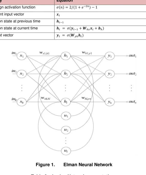
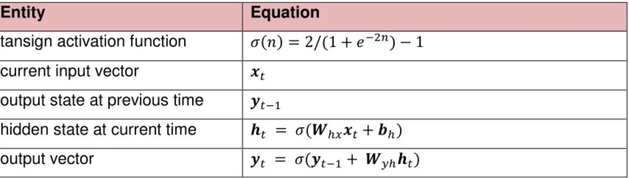
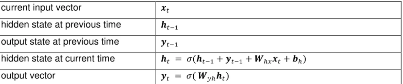
Both the Elman and Jordan neural networks represent special cases of the general class of RNN architecture, comprising input, hidden, and output layers of units, with the addition of weighted delay lines, known as context units, connected to either the hidden or output layer. The context units are a key feature of these networks, copying previous outputs back to the layer units for use with current processing. The architectures for the Elman and Jordan networks are illustrated in Figures 1 and 2, respectively, with equations listed in Tables 1 and 2. As can be seen, both networks are equipped with context units, with the sole difference that the Jordan network has connections at the output layer as opposed to the hidden layer. In addition to these network types, we also introduce for experimentation a hybrid network, where the context units from both the Elman and Jordan network are simultaneously incorporated into a single model, using the connections of both. The hybrid architecture is demonstrated in Figure 3, with equations for the network computation listed in Table 3.
Similarly to other types of neural network, for the architectures considered in this study, the units at the input do not perform computation and serve only to distribute the input values to subsequent layers. Additionally, Elman and Jordan networks represent universal approximators, capable of estimating any numerical function within an arbitrary degree of accuracy, given a sufficient number of units within the hidden layer. In accord with the class of RNN models, Elman and Jordan networks are also theoretically capable of universal computation (Turing completeness) [50-52], since the current links provide additional operational capabilities beyond the reach of feedforward neural networks, for example
looping provision. Consequently, the hybrid Elman-Jordan network is also a universal approximator, due to spanning the set of Turing primitive operations.
Table 1. Elman Network computations
Entity Equation
tansign activation function � � = / + �− − current input vector �
hidden state at previous time ��−
hidden state at current time �� = � �− + �ℎ �+ �ℎ output vector � = � � ℎ��
Figure 1. Elman Neural Network Table 2. Jordan Network computations
Entity Equation
tansign activation function � � = / + �− −
current input vector �
output state at previous time �−
hidden state at current time �� = � �ℎ �+ �ℎ
output vector � = � �− + � ℎ��
The Jordan network can be principally defined in terms of the five equations formally described in Table 2. The network is composed of computational units, each of which transforms presented inputs according to an activation function, in this case the tansig function. Data flows into the network in the form of the current input vector, where it is mapped to an output vector according to both the connection weights between computational units and the dynamical influence of previous inputs.
Figure 2. Jordan Neural Network Table 3. Hybrid Network computations
Entity Equation
current input vector � hidden state at previous time ��− output state at previous time �−
hidden state at current time �� = � ��− + �− + �ℎ �+ �ℎ output vector � = � � ℎ��
The Elman network can be principally defined in terms of the six equations formally described in Table 3. The network is composed of computational units, each of which maps presented inputs according to an activation function, in this case the tansig function. Data flows into the network in the form of the current input vector, where it is mapped to an output vector according to both the connection weights between computational units and the dynamical influence of previous inputs and outputs.
Figure 3. Hybrid Neural Network 4. Methodology
Most studies in the field of machine learning algorithms have been constructed to predict the severe crises of sickle cell disease, in contrast to using advanced predication to determine accurate amounts of a drug called
hydroxyurea/hydroxycarbamide, which is used to modify the disease phenotype [15, 53, 54]. Currently there is no standardisation for disease modifying therapy management. Using the proposed computerised comprehensive management system, the aim is to produce an optimised and reproducible standard of care in different clinical settings across the UK, and indeed internationally. The main backbone of this research is to use recent advances in neural network models, in order to assist healthcare professionals in offering accurate amounts of medication for each individual patient according to their condition. In this case, and due to the pattern of the SCD dataset, we attempt to propose classification of the patient’s data set records at an earlier stage, according to how much of a dose the patient will need to take. This can potentially lower costs, avoiding unnecessary admission to hospitals or special institutions, improving patient welfare and mitigate patient illness before it gets worse over time, particularly with elderly people, and unnecessary interventions.
In this research, we attempt to tackle the problem of a certain symptom that affects SCD patients depending on medical measurements with a predictive classification perspective. Machine learning approaches can be used to build strong classifiers to utilise training and testing datasets, involving past observed cases that have been collected from Liverpool Centre for Sickle Cell Disease in the UK over the last five years. In this case, we examine the performance of current machine learning algorithms such as neural networks for constructing predictive models.
4.1. Data Collection
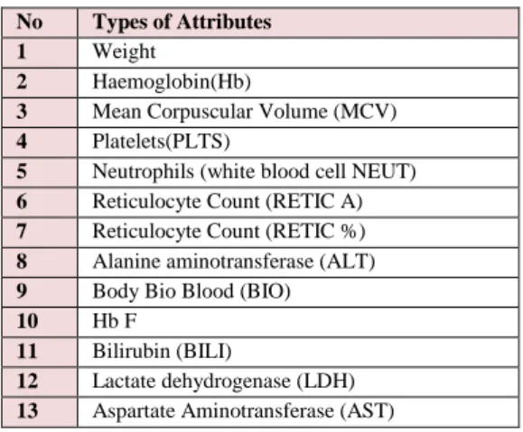
The dataset utilised in our experiments for SCD patients was commissioned specifically for the purposes of this study and was collected within a five-year period from the Alder Hey Children’s hospital based in Liverpool, UK. Each sample comprises 13 attributes deemed vital factors for predicting the SCD trait as illustrated in Table 4. Furthermore, there are two features that should be considered when analysing blood test, which are gender and age [55]. These features have significant effects on the blood test. In order to work with a large amount of data, a local hospital has supported this research with a number of patient records. The resulting dataset comprises 1168 sample points, with a
single target variable describing the hydroxyurea/hydroxycarbamide medication dosage in milligrams. To facilitate our classification study, the target dosage was discretised into 3 bins, denoted classes 1 through 3, formed through dividing the output range (in Milligrams) into membership intervals of equal size: Class 1: [300 ≤ Y < 533mg], Class 2: [533 ≤ Y < 766mg], Class 3: [766 ≤ Y ≤ 1000mg]. Such a division was conducted in order to provide adequate class representation over the data sample, while preserving some level of precision for the dosage outcome. The decision represents a trade-off, since our data sample was limited to one hundred examples, thereby excluding the possibility of a reasonable division for more than three classes.
Table 4. Characteristics of SCD Datasets No Types of Attributes
1 Weight
2 Haemoglobin(Hb)
3 Mean Corpuscular Volume (MCV)
4 Platelets(PLTS)
5 Neutrophils (white blood cell NEUT)
6 Reticulocyte Count (RETIC A)
7 Reticulocyte Count (RETIC %)
8 Alanine aminotransferase (ALT)
9 Body Bio Blood (BIO)
10 Hb F
11 Bilirubin (BILI)
12 Lactate dehydrogenase (LDH)
13 Aspartate Aminotransferase (AST)
4.2. Experimental Setup
In this section, we cover the design of the test environment used in our experiments and the models tested, the configuration of each model, and finally the performance evaluation metrics used to measure the outcomes of the machine learning models for SCD data set.
In order to comprehensively test the capability of the models in our study, we applied several competing models to the same classification task, contrasted with a random oracle model (ROM) [56] to serve as a baseline indicator. Moreover, we introduced a linear model to examine the differential in performance present between this weak classifier and the non-linear classifiers, such as neural networks. The combination of strong, weak, and random control baselines provides an empirical frame of reference through which to gauge the
relative performance of the RNNs. We note also that such a set of reference controls is useful to justify the integrity of the results obtained, since it can be shown that such performance cannot be reached through either the linear model or by random guessing.
Holdout method is used in these experiments for assessing how the outcomes of a statistical analysis could generalise to an independent datasets. The proportion of the dataset is divided into three parts training, validation, and testing phases. This study used the holdout method of data partitioning to find an average percentage of the correct classifications. The training set receives 70 % of the available data, the validation set 10%, while the testing set is allocated the remaining 20%. The division of data between separate training and testing sets ensures that the generalisation error of the models can be assessed, demonstrating the ability of classifiers to operate on unseen data.
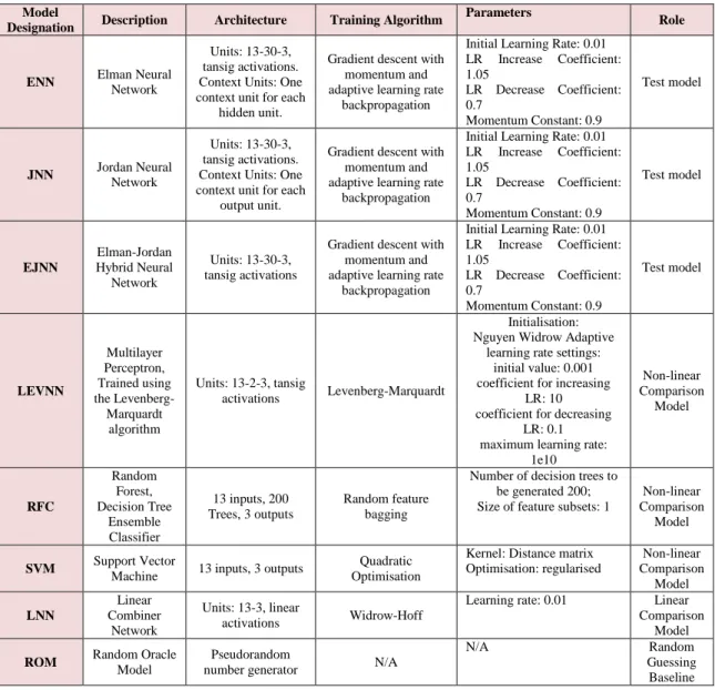
The models under study are composed of three types of RNNs: the Elman Neural Network Classifier (ENNC), the Jordan Neural Network Classifier (JNNC), and hybrid RNN, where both the Elman and Jordan connections are combined within a single model (EJNNC). Other model set is composed of a multi-layer perceptron, trained using the Levenberg-Marquardt learning algorithm (LEVNN), random forest classifier (RFC), and support vector machine classifier (SVM). These models are considered strong non-linear classifiers and are suitable to act as comparators of high performance. The linear model we used comprises a single layer neural network with a linear transformation function at each class output unit. Finally, we used random oracle model (ROM) to establish random case performance through the assignment of random responses for each class. To obtain performance estimates for the respective models, we ran each simulation 50 times and calculates the mean of the responses. The full set of models used in the experiments are described in Table 5.
Table 5. Classification Models Model
Designation Description Architecture Training Algorithm
Parameters
Role
ENN Elman Neural Network
Units: 13-30-3, tansig activations. Context Units: One context unit for each
hidden unit.
Gradient descent with momentum and adaptive learning rate
backpropagation
Initial Learning Rate: 0.01 LR Increase Coefficient: 1.05 LR Decrease Coefficient: 0.7 Momentum Constant: 0.9 Test model JNN Jordan Neural Network Units: 13-30-3, tansig activations. Context Units: One context unit for each
output unit.
Gradient descent with momentum and adaptive learning rate
backpropagation
Initial Learning Rate: 0.01 LR Increase Coefficient: 1.05 LR Decrease Coefficient: 0.7 Momentum Constant: 0.9 Test model EJNN Elman-Jordan Hybrid Neural Network Units: 13-30-3, tansig activations
Gradient descent with momentum and adaptive learning rate
backpropagation
Initial Learning Rate: 0.01 LR Increase Coefficient: 1.05 LR Decrease Coefficient: 0.7 Momentum Constant: 0.9 Test model LEVNN Multilayer Perceptron, Trained using the Levenberg-Marquardt algorithm Units: 13-2-3, tansig activations Levenberg-Marquardt Initialisation: Nguyen Widrow Adaptive
learning rate settings: initial value: 0.001 coefficient for increasing
LR: 10 coefficient for decreasing
LR: 0.1 maximum learning rate:
1e10 Non-linear Comparison Model RFC Random Forest, Decision Tree Ensemble Classifier 13 inputs, 200 Trees, 3 outputs Random feature bagging
Number of decision trees to be generated 200; Size of feature subsets: 1
Non-linear Comparison
Model
SVM Support Vector
Machine 13 inputs, 3 outputs
Quadratic Optimisation
Kernel: Distance matrix Optimisation: regularised Non-linear Comparison Model LNN Linear Combiner Network Units: 13-3, linear activations Widrow-Hoff
Learning rate: 0.01 Linear Comparison
Model
ROM Random Oracle Model number generator Pseudorandom N/A
N/A Random Guessing Baseline
Metric Name Calculation
Sensitivity TP/(TP+FN)
Specificity TN/(TN+FP)
Precision TP/(TP+FP)
F1 Score 2 * (Precision*Recall)/(Precision+Recall) Youden's J statistic (J Score) Sensitivity + Specificity − 1
Accuracy (TP+TN)/(TP+FN+TN+FP)
Area Under ROC Curve
(AUC) 0 <= Area under the ROC Curve <= 1
Our model evaluation framework consists of both in-sample (training) and out-of-sample (testing) diagnostics, comprising sensitivity, specificity, precision, the F1 score, Youden’s J statistic, and overall classification accuracy calculated as shown in Table 6. Additionally, the classifiers are characterised using ROC plots and the area under the curve (AUC), where the classification ability across all operating points is ascertained.
5. Results Evaluation
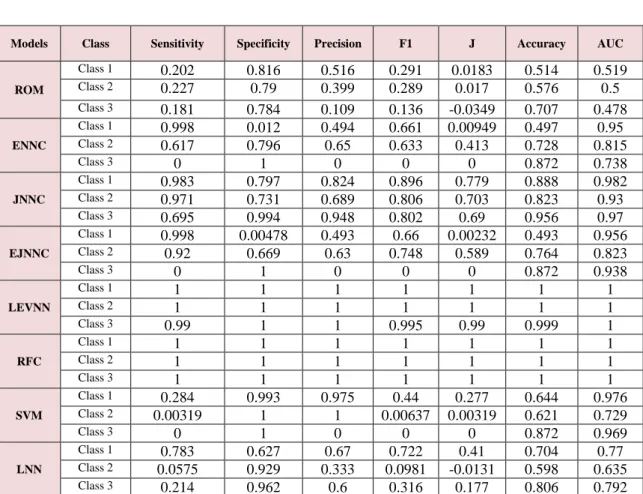
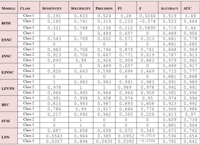
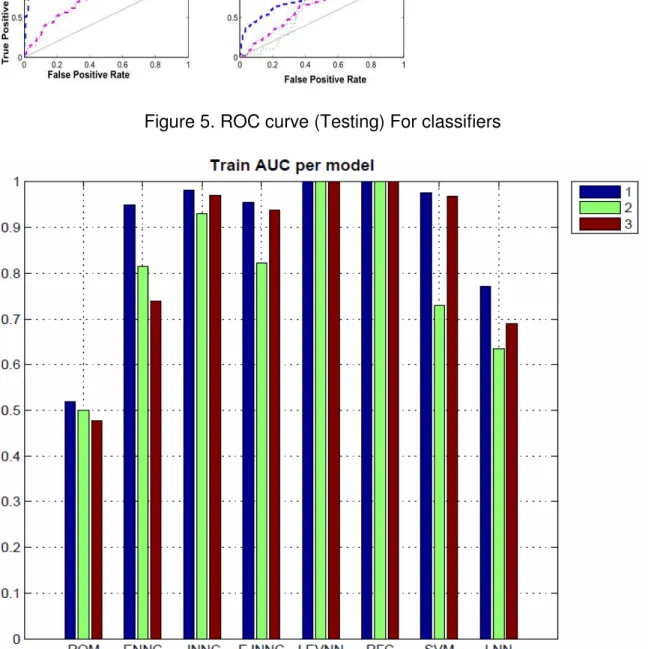
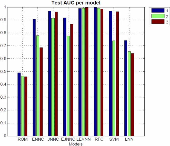
The results from our experiments are listed in Tables 7 and 8, showing outcomes for training and testing of the classifiers, respectively. We also provide further performance visualisations through the use of ROC plots (Figures 4 and 5) and the use of AUC plots as illustrated in Figures 6 and 7. The AUC bar graphs provide a visual comparison of the area under the ROC curve across the models tested.
The results obtained from the experiments show that the LEVNN and RFC classifiers outperformed all other classifiers, including the RNNs, by a significant margin. Both classifiers achieve an ideal fit over the trainings set for all operating points, as can be illustrated in Table 7 and the ROC and AUC plots shown in Figures 4 and 6, respectively. Moreover, the performance obtained during the training of these two classifiers is shown to provide excellent generalisation to the test set, with AUCs ranging between 0.986 to 0.996. The strong generalisation of these two classifiers indicates that there exists rich information
content embedded within our selected data source, showing a high upper bound on classification performance. We conducted further experiments using SVM classifier, showing that this class of model is significantly less capable for classifying our dataset.
Further experiments show that the chosen dataset exhibits significant non-linear relationships, presenting a challenge for RNN test models. Of the RNN classifiers under study, the Jordan network outperformed the Elman and Elman-Jordan hybrid, demonstrating capability both for fitting the training data and also in generalising to unseen examples. The AUCs obtained for the Jordan model during training are 0.982, 0.93, and 0.97 for classes 1 to 3 respectively, in comparison to 0.969, 0.913, and 0.962 over the test sample. Subsequently, a single operating point was selected to illustrate a final classification decision; it was found that the performance at the chosen rejection threshold varied between the training and testing sets for Class 2, as reflected earlier in the AUC values. Classes 1 and 3 were found to show reasonably consistent performance representation between the train and test sets for this model. It is possible that the reasonable performance obtained for the JNN architecture, in contrast with the poor performance of the other RNN types, could point to a detrimental effect caused by presence of feedbacks from the hidden layer outputs in the classification setting. The final layer output feedbacks present in the JNN model, appear not to negatively impact learning.
The Elman and Elman-Jordan RNNs are found to perform similarly to one another, with both ranking below the JNN for both the training and testing sets. The AUC values for both models ranged between 0.738, and 1 in respect to the training set, and 0.685 to 0.906 for the testing procedure. Consistent with the results obtained from the JNN, it was found that the outcomes for Class 2 show the largest differential between the training and testing sets. On further examination of the results from the ENN and EJNN, it was found that despite the appearance of reasonable AUC values during training, the networks had converged to a particularly narrow output range, suggesting that the training process is unable to achieve clear correspondence with the classification targets, arriving instead at marginal responses. Further confirmation is reflected in the sensitivities and specificities obtained for these two models, with values seen to
fluctuate between opposite extremes. Such a situation stands in contrasted with the JNN model, for which a reasonable range of output values is achieved during both train and test phases. It is noted that for both the ENN and EJNN, the operation of the hidden layer is altered using recurrent links, whereas the JNN hidden layer is altered via feedback from the output layer.
It is shown that the model does not generalise well from training to testing, producing reasonable AUCs for in-sample fitting, while yielding test set AUCs little better than the LNN baseline. The test AUCs for this model ranged between 0.49 and 0.46. As expected, the LNN was unable to learn the non-linear components in the data and so produces weak classification results against which the other classifiers can be contrasted. The ROM is seen to follow the diagonal of the ROC plots for all classes (see Figure 4 and 5), illustrating by contrast the significance of the results from the other trained classifiers.
Table 7. Comparison Table for Classifiers (Training)
Models Class Sensitivity Specificity Precision F1 J Accuracy AUC
ROM Class 1 0.202 0.816 0.516 0.291 0.0183 0.514 0.519 Class 2 0.227 0.79 0.399 0.289 0.017 0.576 0.5 Class 3 0.181 0.784 0.109 0.136 -0.0349 0.707 0.478 ENNC Class 1 0.998 0.012 0.494 0.661 0.00949 0.497 0.95 Class 2 0.617 0.796 0.65 0.633 0.413 0.728 0.815 Class 3 0 1 0 0 0 0.872 0.738 JNNC Class 1 0.983 0.797 0.824 0.896 0.779 0.888 0.982 Class 2 0.971 0.731 0.689 0.806 0.703 0.823 0.93 Class 3 0.695 0.994 0.948 0.802 0.69 0.956 0.97 EJNNC Class 1 0.998 0.00478 0.493 0.66 0.00232 0.493 0.956 Class 2 0.92 0.669 0.63 0.748 0.589 0.764 0.823 Class 3 0 1 0 0 0 0.872 0.938 LEVNN Class 1 1 1 1 1 1 1 1 Class 2 1 1 1 1 1 1 1 Class 3 0.99 1 1 0.995 0.99 0.999 1 RFC Class 1 1 1 1 1 1 1 1 Class 2 1 1 1 1 1 1 1 Class 3 1 1 1 1 1 1 1 SVM Class 1 0.284 0.993 0.975 0.44 0.277 0.644 0.976 Class 2 0.00319 1 1 0.00637 0.00319 0.621 0.729 Class 3 0 1 0 0 0 0.872 0.969 LNN Class 1 0.783 0.627 0.67 0.722 0.41 0.704 0.77 Class 2 0.0575 0.929 0.333 0.0981 -0.0131 0.598 0.635 Class 3 0.214 0.962 0.6 0.316 0.177 0.806 0.792
MODELS CLASS SENSITIVITY SPECIFICITY PRECISION F1 J ACCURACY AUC ROM Class 1 0.191 0.833 0.524 0.28 0.0246 0.519 0.49 Class 2 0.185 0.741 0.315 0.233 -0.074 0.523 0.464 Class 3 0.321 0.768 0.158 0.212 0.0895 0.715 0.46 ENNC Class 1 1 0 0.489 0.657 0 0.489 0.906 Class 2 0.543 0.769 0.602 0.571 0.313 0.681 0.778 Class 3 0 1 0 0 0 0.881 0.685 JNNC Class 1 0.983 0.758 0.796 0.879 0.741 0.868 0.969 Class 2 0.913 0.706 0.667 0.771 0.619 0.787 0.913 Class 3 0.893 0.99 0.926 0.909 0.883 0.979 0.962 EJNNC Class 1 1 0 0.489 0.657 0 0.489 0.917 Class 2 0.826 0.643 0.598 0.694 0.469 0.715 0.777 Class 3 0 1 0 0 0 0.881 0.868 LEVNN Class 1 1 0.983 0.983 0.991 0.983 0.991 0.989 Class 2 0.978 1 1 0.989 0.978 0.991 0.991 Class 3 0.964 0.995 0.964 0.964 0.959 0.991 0.996 RFC Class 1 0.991 0.958 0.958 0.974 0.95 0.974 0.996 Class 2 0.815 0.993 0.987 0.893 0.808 0.923 0.992 Class 3 0.786 0.99 0.917 0.846 0.776 0.966 0.986 SVM Class 1 0.217 0.992 0.962 0.355 0.209 0.613 0.97 Class 2 0 1 0 0 0 0.609 0.739 Class 3 0 1 0 0 0 0.881 0.964 LNN Class 1 0.687 0.658 0.658 0.672 0.345 0.672 0.742 Class 2 0.0543 0.944 0.385 0.0952 -0.0016 0.596 0.654 Class 3 0.0357 0.894 0.0435 0.0392 -0.0706 0.791 0.641
Figure 5. ROC curve (Testing) For classifiers
The plots show in Figures 6 and 7 show the area under the ROC curve (AUC) for each class over each model within our experiment. Figure 6 shows the results obtained for the training set and Figure 7 the test set, respectively. The AUC value is a scalar summary used to characterise the global capability of a given classifier under study. In our plots, the X axis shows the models and classes, while the Y axis shows the AUC that corresponds to each of the model entries listed over the X axis. An AUC of 1 represents an ideal classifier, while an AUC of 0.5 represents random performance. Each of the bars plotted is associated with a corresponding curve in either of Figures 4 and 5, which represent the accompanying ROC curves for the training and testing sets. The purpose of the plot is to emphasise the AUC values in graphical form, such that a visual comparison can be drawn.
Overall, the body of results that we obtained highlight the potential of medical data for the classification of SCD dosage ranges. It is clear that the choice of model is crucial in obtaining a satisfactory result, as is evident in the variation of the performance between the models used in our experiment. The LEVNN and RFC classifiers responded successfully to the SCD data and are therefore of potential use in the medical field.
6. Conclusion and Future works
In this study, we have conducted an empirical investigation into the use of various types of machine learning models for the classification of SCD effective dosage levels. This paper has introduced various types of recurrent neural network for the purpose of analysing medical time series obtained from SCD patients in contrast with traditional medical solutions. Previous studies have demonstrated that Machine learning models exhibit considerable effectiveness for the pre-processing of medical time-series data signals as a precursor to the classification of medical data. Our study sought to investigate the effectiveness of machine learning approach including ANNs when posed in the direct classification setting for classification of SCD effective dosage levels. It was found through empirical investigation, involving the use of patient sample data and comparator models such as SVM and RFC, that RNNs, although capable of providing some degree of fitting and generalisation, are suboptimal in the classification setting within our experiment. We consider for future work the use of global optimisation algorithms such as genetic optimisation to explore more comprehensively the space of possible recurrent network architectures. We note that the current study has addressed only a limited set of architectures, which may not expose the full potential of the RNNs within the classification setting; we suggest therefore that an algorithmic model search may be used to expand the scope and scale of this study.
References
[1] P. Sebastiani, M.F. Ramoni, V. Nolan, C.T. Baldwin, M.H. Steinberg, Genetic dissection and prognostic modeling of overt stroke in sickle cell anemia, Nat Genet, 37 (2005) 435-440.
[2] D.J. Weatherall, The importance of micromapping the gene frequencies for the common inherited disorders of haemoglobin, British journal of haematology, 149 (2010) 635-637.
[3] D.J. Weatherall, The inherited diseases of hemoglobin are an emerging global health burden, Blood, (2010).
[4] B.E. Gee, Biologic complexity in sickle cell disease: implications for developing targeted therapeutics, The Scientific World Journal, 2013 (2013).
[5] A. Eleftheriou, M. Angastiniotis, D. Loukopoulos, C. Kattamis, J. Meletis, 3rd Pan-European Conference on Haemoglobinopathies and Rare Anaemias, 24-26 October 2012, Limassol-Cyprus, Thalassemia Reports, 2 (2012) 1-41.
[6] J. de la Fuente, A. Mohammed, Prevalence Of Nocurnal Enuresis and Proteinuria In Children With Sickle Cell Disease and Its Relation To Severity Of Painful Crises, Blood, 122 (2013) 4693-4693.
[7] R. Galanello, R. Origa, Review: beta-thalassemia, Orphanet J Rare Dis, 5 (2010). [8] S.A. Scott, L. Edelmann, L. Liu, M. Luo, R.J. Desnick, R. Kornreich, Experience with carrier screening and prenatal diagnosis for 16 Ashkenazi Jewish genetic diseases, Human mutation, 31 (2010) 1240-1250.
[9] L. Gort, N. de Olano, J. Macías-Vidal, M.J. Coll, S.G.W. Group, GM2 gangliosidoses in
Spain: Analysis of the HEXA and HEXB genes in 34 Tay–Sachs and 14 Sandhoff patients,
Gene, 506 (2012) 25-30.
[10] M. Kosaryan, H. Karami, M. Zafari, N. Yaghobi, Report on patients with non
transfusion-depe de t β-thalassemia major being treated with hydroxyurea attending
the Thalassemia Research Center, Sari, Mazandaran Province, Islamic Republic of Iran in 2013, Hemoglobin, 38 (2014) 115-118.
[11] H. Adams, Medical Informatics: Computer Applications in Health Care, JAMA, 265 (1991) 522-522.
[12] M. Taiana, J. Nascimento, A. Bernardino, On the purity of training and testing data for learning: The case of pedestrian detection, Neurocomputing, 150 (2015) 214-226. [13] R. Strasser, Rural health around the world: challenges and solutions, Family practice, 20 (2003) 457-463.
[14] G.D. Magoulas, A. Prentza, Machine learning in medical applications, Machine Learning and its applications, (Springer, 2001), pp. 300-307.
[15] C. Allayous, S. Clémençon, B. Diagne, R. Emilion, T. Marianne, Machine Learning Algorithms for Predicting Severe Crises of Sickle Cell Disease, (2008).
[16] A.V. Solanki, Data Mining Techniques Using WEKA classification for Sickle Cell Disease”, IJCSIT) I ter atio al Jour al of Co puter S ie e a d I for atio Technologies, 5 (2014) 5857-5860.
[17] M. Seera, C.P. Lim, A hybrid intelligent system for medical data classification, Expert Systems with Applications, 41 (2014) 2239-2249.
[18] D.-S. Huang, C.-H. Zheng, Independent component analysis-based penalized discriminant method for tumor classification using gene expression data, Bioinformatics, 22 (2006) 1855-1862.
[19] M.F. Akay, Support vector machines combined with feature selection for breast cancer diagnosis, Expert systems with applications, 36 (2009) 3240-3247.
[20] L. Ohno-Machado, Medical applications of artificial neural networks: connectionist models of survival, Stanford University, 1996.
[21] H. De-Shuang, D. Ji-xiang, A Constructive Hybrid Structure Optimization Methodology for Radial Basis Probabilistic Neural Networks, Neural Networks, IEEE Transactions on, 19 (2008) 2099-2115.
[22] X. Chen, X. Zhu, D. Zhang, A discriminant bispectrum feature for surface electromyogram signal classification, Medical Engineering and Physics, 32 126-135. [23] A. Graves, A.R. Mohamed, G. Hinton, Speech recognition with deep recurrent neural networks, Acoustics, Speech and Signal Processing (ICASSP), 2013 IEEE International Conference on2013), pp. 6645-6649.
[24] X. Chen, X. Zhu, D. Zhang, A discriminant bispectrum feature for surface electromyogram signal classification, Medical engineering & physics, 32 (2010) 126-135. [25] G.P. Zhang, Neural networks for classification: a survey, Systems, Man, and Cybernetics, Part C: Applications and Reviews, IEEE Transactions on, 30 (2000) 451-462. [26] N.F. Güler, E.D. Ü eyli, İ. Güler, Re urre t eural etworks employing Lyapunov exponents for EEG signals classification, Expert Systems with Applications, 29 (2005) 506-514.
[27] P. Fergus, I. Idowu, A. Hussain, C. Dobbins, Advanced artificial neural network classification for detecting preterm births using EHG records, Neurocomputing, 188 (2016) 42-49.
[28] E.H. Shortliffe, J.J. Cimino, Biomedical informatics: computer applications in health care and biomedicine (Springer Science & Business Media, 2013).
[29] T.K. Ho, The random subspace method for constructing decision forests, Pattern Analysis and Machine Intelligence, IEEE Transactions on, 20 (1998) 832-844.
[30] T.K. Ho, Random decision forests, Document Analysis and Recognition, 1995., Proceedings of the Third International Conference on, (IEEE1995), pp. 278-282.
[31] L. Breiman, Random forests, Machine learning, 45 (2001) 5-32.
[32] T.K. Ho, A data complexity analysis of comparative advantages of decision forest constructors, Pattern Analysis & Applications, 5 (2002) 102-112.
[33] C. Cortes, V. Vapnik, Support-vector networks, Machine learning, 20 (1995) 273-297.
[34] V. Vapnik, The nature of statistical learning theory (Springer Science & Business Media, 2013).
[35] Y. Liu, X. Yu, J.X. Huang, A. An, Combining integrated sampling with SVM ensembles for learning from imbalanced datasets, Information Processing & Management, 47 (2011) 617-631.
[36] F. Amato, A. Lopez, E.M. Peña-Mé dez, P. Vaňhara, A. Ha pl, J. Havel, Artifi ial
neural networks in medical diagnosis, Journal of applied biomedicine, 11 (2013) 47-58. [37] A.J. Maren, C.T. Harston, R.M. Pap, Handbook of neural computing applications (Academic Press, 2014).
[38] A. Wu, S. Wen, Z. Zeng, Synchronization control of a class of memristor-based recurrent neural networks, Information Sciences, 183 (2012) 106-116.
[39] E.D. Übeyli, M. Übeyli, Case Studies for Applications of Elman Recurrent Neural Networks, (Recurrent Neural Networks,(Eds.) Xiolin Hu y P. Balasubramaniam. Editorial INTECH2008).
[40] A. Petrosian, D. Prokhorov, W. Lajara-Nanson, R. Schiffer, Recurrent neural network-based approach for early recognition of Alzheimer's disease in EEG, Clinical Neurophysiology, 112 (2001) 1378-1387.
[41] A. Petrosian, D. Prokhorov, R. Homan, R. Dasheiff, D. Wunsch Ii, Recurrent neural network based prediction of epileptic seizures in intra- and extracranial EEG, Neurocomputing, 30 (2000) 201-218.
[42] F. Visin, K. Kastner, K. Cho, M. Matteucci, A. Courville, Y. Bengio, ReNet: A Recurrent Neural Network Based Alternative to Convolutional Networks, arXiv preprint arXiv:1505.00393, (2015).
[43] E.D. Übeyli, Analysis of EEG signals by implementing eigenvector methods/recurrent neural networks, Digital Signal Processing, 19 (2009) 134-143.
[44] M. Hüsken, P. Stagge, Recurrent neural networks for time series classification, Neurocomputing, 50 (2003) 223-235.
[45] S. Haykin, N. Network, A comprehensive foundation, Neural Networks, 2 (2004). [46] J.R. Chung, J. Kwon, Y. Choe, Evolution of recollection and prediction in neural networks, Neural Networks, 2009. IJCNN 2009. International Joint Conference on, (IEEE2009), pp. 571-577.
[47] V.A. Makarov, Y. Song, M.G. Velarde, D. Hübner, H. Cruse, Elements for a general memory structure: properties of recurrent neural networks used to form situation models, Biological cybernetics, 98 (2008) 371-395.
[48] S. Ling, F.H. Leung, K. Leung, H. Lam, H. Iu, An improved GA based modified dynamic neural network for Cantonese-digit speech recognition (InTech Open Access Publisher, 2007).
[49] E.M. Forney, C.W. Anderson, Classification of EEG during imagined mental tasks by forecasting with Elman recurrent neural networks, Neural Networks (IJCNN), The 2011 International Joint Conference on, (IEEE2011), pp. 2749-2755.
[50] H.T. Siegelmann, E.D. Sontag, On the Computational Power of Neural Nets, Journal of Computer and System Sciences, 50 (1995) 132-150.
[51] H.T. Siegelmann, B.G. Horne, C.L. Giles, Computational capabilities of recurrent NARX neural networks, Systems, Man, and Cybernetics, Part B: Cybernetics, IEEE Transactions on, 27 (1997) 208-215.
[52] H. Siegelmann, Neural networks and analog computation: beyond the Turing limit (Springer Science & Business Media, 2012).
[53] M. Khalaf, A.J. Hussain, D. Al-Jumeily, R. Keenan, P. Fergus, I.O. Idowu, Robust Approach for Medical Data Classification and Deploying Self-Care Management System for Sickle Cell Disease, Computer and Information Technology; Ubiquitous Computing and Communications; Dependable, Autonomic and Secure Computing; Pervasive Intelligence and Computing (CIT/IUCC/DASC/PICOM), 2015 IEEE International Conference on2015), pp. 575-580.
[54] A.V. Solanki, Data Mining Techniques Using WEKA classification for Sickle Cell Disease, International Journal of Computer Science and Information Technologies, 5 (2014) 5857-5860.
[55] F. Parent, D. Bachir, J. Inamo, F. Lionnet, F. Driss, G. Loko, A. Habibi, S. Bennani, L. Savale, S. Adnot, B. Maitre, A. Yaïci, L. Hajji, D.S. O'Callaghan, P. Clerson, R. Girot, F. Galacteros, G. Simonneau, A Hemodynamic Study of Pulmonary Hypertension in Sickle Cell Disease, New England Journal of Medicine, 365 (2011) 44-53.
[56] X.-Y. Jia, B. Li, Y.-M. Liu, Random oracle model, Ruanjian Xuebao/Journal of Software, 23 (2012) 140-151.