A New Method for Outlier Detection on Time Series Data

(1)

A New Method for Outlier Detection on Time Series Data

by

Lin Liu

M.Eng., Beijing University of Posts and Telecommunications, 2013 B.Eng., Minzu University of China, 2010

a Thesis submitted in partial fulfillment of the requirements for the degree of

Master of Science in the

School of Computing Science Faculty of Applied Sciences

c

Lin Liu 2015

SIMON FRASER UNIVERSITY Summer 2015

However, in accordance with theCopyright Act of Canada, this work may be reproduced without authorization under the conditions for “Fair Dealing.” Therefore, limited reproduction of this work for the purposes of private study,

research, criticism, review and news reporting is likely to be in accordance with the law, particularly if cited appropriately.

(2)

APPROVAL

Name: Lin Liu

Degree: Master of Science

Title of Thesis: A New Method for Outlier Detection on Time Series Data

Examining Committee: Dr. Arrvindh Shriraman, Assistant Professor, Chair

Dr. Jian Pei,

Professor, Senior Supervisor

Dr. Qianping Gu, Professor, Supervisor

Dr. Jiangchuan Liu,

Professor, External Examiner

Date Approved: June 9th, 2015

(3)

Abstract

Time series outlier detection has been attracting a lot of attention in research and appli-cation. In this thesis, we introduce the new problem of detecting hybrid outliers on time series data. Hybrid outliers show their outlyingness in two ways. First, they may deviate greatly from their neighbors. Second, their behaviors may also be different from that of their peers in other time series. We propose a framework to detect hybrid outliers, and two algorithms based on the framework are developed to show the feasibility of our framework. An extensive empirical study on both real data and synthetic data verifies the effectiveness and efficiency of our algorithms.

Keywords: Outlier detection; time series; hybrid outlier; distance; prediction

(4)

To my family.

(5)

“The only true wisdom is in knowing you know nothing.” —Socrates, (470 - 399 BC)

(6)

Acknowledgments

I would like to express my sincerest gratitude to my senior supervisor, Dr. Jian Pei, for his great patience, wealth of knowledge, warm encouragement and continuous support through-out my Master’s studies. He taught me not only valuable knowledge, but also the wisdom of life, which gave me interest and confidence in accomplishing this thesis.

I am very thankful to Dr. Qianping Gu for being my supervisor and giving me helpful suggestions that helped me to improve my thesis. I am also grateful to thank Dr. Jiangchuan Liu and Dr. Arrvindh Shriraman for serving in my examining committee.

My deepest thanks to Professor Jiali Bian and Professor Jian Kuang in Beijing University of Posts and Telecommunications for educating and training me for my career.

I thank Dr. Huaizhong Lin, Dr. Aihua Wu, Dr. Fuyuan Cao, Dr. Kui Yu, Dr. Dongwan Choi, Dr. Guanting Tang, Xiao Meng, Juhua Hu, Xiangbo Mao, Chuancong Gao, Xiaoning Xu, Yu Tao, Xuefei Li, Yu Yang, Jiaxing Liang, Beier Lu, Li Xiong, Lumin Zhang, Xiang Wang, Zicun Cong, and Xiaojian Wang for their kind help during my study at SFU. I am also grateful to my friends at Fortinet. I thank Kai Xu, for his guide and insight suggestions. Last but not least, I am very grateful to my parents, my husband, my sister, and my brother, for their endless love and support through all these years. Without them, never can I accomplish this thesis.

(7)

List of Tables

3.1 The summary of symbols . . . 13

3.2 Notations used in the algorithm framework . . . 15

3.3 2-NN segments during iterations . . . 18

3.4 The outlier degree rank of time points during iterations . . . 18

4.1 Notations used in the distance-based algorithm . . . 22

4.2 Three time series . . . 22

4.3 Notations used in the prediction-based algorithm . . . 24

4.4 2-NN segments during iterations for DA . . . 27

4.5 Outlier score of each time point during iterations for DA . . . 27

4.6 Distance weight of each time point during iterations for DA . . . 27

4.7 Final outlier degree rank of time points for DA . . . 28

4.8 2-NN segments during iterations for PA . . . 28

4.9 Outlier scores of time points during iterations for PA . . . 28

4.10 Distance weight of time points during iterations for PA . . . 29

4.11 Average score of all time point in all time series during iterations for PA . . . 29

4.12 Final outlier degree rank of time points for PA . . . 30

5.1 Top 10 hybrid outliers detected by our two algorithms . . . 32

5.2 Top 10 hybrid outliers detected by the baselines . . . 32

5.3 Top 10 self-trend and peer-wise outliers . . . 33

5.4 The description of 4 real data sets . . . 35

5.5 Original time series . . . 36

5.6 Synthetic time series . . . 36

(10)

List of Figures

2.1 4 time series data . . . 6

3.1 An example of time series . . . 10

3.2 Small time series data . . . 12

3.3 Overview of the framework . . . 14

5.1 Results on the real data set (w = 5, k = 4) . . . 34

5.2 Monthly exchange rates of 7 currencies w.r.t. USD . . . 39

5.3 Results on synthetic temperature data set . . . 40

5.4 Results on synthetic exchange rate data set . . . 41

5.5 Results on synthetic interest rate data set . . . 42

5.6 Results on synthetic government GDP data set . . . 43

5.7 Results of DA on 4 synthetic data sets with respect to r (x=4, y=40, k=5, w=6) . . . 44

(11)

Chapter 1

Introduction

In this chapter, we first discuss several interesting applications that motivate the problem of hybrid outlier detection on time series data, which will be studied in this thesis. Then, we will summarize the major contributions and describe the structure of the thesis.

1.1 Motivations

Time series data are becoming increasingly important in many areas, such as finance, signal processing, and weather forecasting. Time series data are observations collected sequentially over time. Some examples of time series data are the daily stock price of a firm, the daily temperature for a region, the altitude of an airplane every second, the exchange rate of a currency every month, and so on. In all these instances, a measure is associated with a timestamp. By analyzing time series data, people can extract useful information from the data and gain insight into the data.

Despite the large amounts of data, people are very interested in unusual values (or outliers) out of the whole time series data. Usually time series outliers are informally defined as somehow unexpected or surprising values in relation to the rest of the series, often the immediately preceding and following observations [37]. A great number of methods have been proposed to detect different types of time series outliers, and most of the existing methods work on detecting outlier points or subsequences in a single time series [20] [21] [38] or finding entire time series as outliers in multiple time series [43] [31] [42].

In this thesis, we pose the new problem of detecting hybrid outliers on time series data. Hybrid outliers show their outlyingness in two ways. First, they may deviate greatly from

(12)

CHAPTER 1. INTRODUCTION 2

their neighbors. Second, their behaviors may also be different from that of their peers in other time series. If two observations in different time series have the same timestamp, they are peers of each other. In general, a hybrid outlier has a combination of self-trend outlier behavior and peer-wise outlier behavior. Hybrid outliers are valuable in various application areas. Some motivating examples are as follows.

Example 1 (Motivation - temperature): Temperature data are a kind of time series data, which are commonly collected in climate and environment research. Anomalies in temperature data provide significant insights about hidden environmental trends, which may have caused such anomalies.

In temperature data, each time series usually represents the temperature values of a geographical region over time, and the time series from close regions are likely to have similar trends. In many cases, the interestingness of a particular temperature value of a region not only depends on its past temperature values, but also depends on the data from close regions. For example, suppose there is a sudden temperature increase in Vancouver, and we know other close regions, like Richmond and Burnaby, do not have temperature rise at the same time, then this temperature change in Vancouver would be very interesting and worth investigation. On the other hand, if the temperature increase in Vancouver is along with the rising temperatures in other close regions, this change would be more likely some common climate trends.

Clearly, outlier detection on time series data from both the self-trend aspect and the

peer-wise aspect is practically useful.

Example 2 (Motivation - exchange rate): The exchange rate of a currency partly reflects the economic health of the country. By analyzing the change of currency exchange rate, people can predict economic trends of the country to some extent. In currency exchange rate data, each time series represents a sequence of exchange rate values (usually with respect to US dollar) of a currency. Some currencies often have similar trends, like GBP (British Pound), EUR (Euro), and CHF (Swiss Franc), because the countries have frequent economic cooperation.

When analyzing the exchange rate of a currency, people are not only interested in the trend with respect to its historical data, but also interested in how the trend is different from those of some other close related currencies. For example, if the exchange rate of GBP drops greatly this month and the exchange rates of EUR and CHF also drop at the same time, then this change is probably caused by some economic problem of the whole European

(13)

CHAPTER 1. INTRODUCTION 3

continent. However, if the GBP is the only currency going down, this change would be more interesting and it deserves to be further analyzed.

Again, outlier detection on time series data from both the self-trend aspect and the

peer-wise aspect is meaningful.

Besides, hybrid outliers are interesting and useful in many other applications, like medi-cal diagnosis, network intrusion detection systems, stock market analysis, interesting sensor events, etc. To the best of our knowledge, there does not exist any systematic study on mining hybrid outliers.

1.2 Contributions

In this thesis, we tackle the problem of hybrid outlier detection on time series data, and make the following contributions.

• We pose the new problem of detecting hybrid outliers.

• We propose a heuristic framework for detecting hybrid outliers.

• We develop two algorithms based on the framework. The first one is a distance-based algorithm and the other one is a prediction-based algorithm.

• We report an empirical evaluation on both synthetic and real-world data sets, which validates the effectiveness and efficiency of our algorithms.

1.3 Organization of the Thesis

The rest of the thesis is organized as follows. In Chapter 2, we review the related work on time series outlier detection. We then formulate the problem ofhybrid outlier detection on time series data and propose our framework in Chapter 3. In Chapter 4, two algorithms based on the framework are presented. We report our experimental results in Chapter 5, and conclude the thesis in Chapter 6.

(14)

Chapter 2

Related Work

A significant amount of work has been performed in the area of time series outlier detection. The existing techniques on time series outlier detection can be divided into two categories: the techniques to detect outliers within a single time series, and the techniques over multiple time series, which are reviewed in Section 2.1 and Section 2.2, respectively.

2.1 Detecting Outliers within a Single Time Series

Given a single time series, an outlier can be either a time point or a subsequence. In this subsection, we will discuss methods for both these cases.

2.1.1 Time Points as Outliers

Various methodologies were proposed to find outlier time points in a time series. Deviant detection and prediction models are two of them.

Deviants are outlier time points in time series from a minimum description length (MDL) point of view [20]. If the removal of a time point from the time series leads to an improved compressed representation of the remaining items, then the point is a deviant [26]. A dy-namic programming mechanism for deviant detection was developed by Jagadishet al. [20]. Muthukrishnanet al. [26] proposed an approximation method to the dynamic programming based solution.

The general idea of prediction models [1] is to predict the value of a time point and compute the deviation from the predicted value to its real value as the outlier score for the

(15)

CHAPTER 2. RELATED WORK 5

time point. Basuet al.[4] predicted the value of the time point at timetas a median of the values of the time points in the size of 2wwindow fromt−w tot+w. Hillet al. [19] used single-layer linear network predictor (or AR model) which predicts the value at time t as a linear combination of the q previous values. A vector auto-regressive integrated moving average (or ARIMA) model was proposed to identify 4 types of outliers from multi-variate time series by Tsayet al.[38]. ARIMA is a traditional and frequently used methodology for time series forecasting, which was first popularized by Box and Jenkins [17]. An ARIMA model predicts a value in a time series as a linear combination of its own past values and past errors.

2.1.2 Subsequences as Outliers

A bunch of methods were proposed to discover discord, which is a type of outlier subse-quences in a time series. Keoghet al. [22] gave the definition of discord: given a time series T, the subsequenceDof lengthnbeginning at positionlis said to be the discord (or outlier) of T if D has the largest distance to its nearest non-overlapping match. The brute force algorithm for finding discord is to consider all possible subsequencess∈S of lengthninT and compute the distance of each suchswith each other non-overlapping s0∈S. To make the computation efficient, effective pruning techniques implemented by smartly ordering subsequence comparisons are used in many methods, like heuristic reordering of candidate subsequences using SAX (HOT SAX) [21], Haar wavelet and augmented tries (WAT) [9], and locality sensitive hashing (LSH) [40].

Chenet al.[12] defined the subsequence outlier detection problem for an unequal interval time series which is a time series with values sampled at unequal time intervals. For such a time series, a pattern is defined as a subsequence of two neighbor points. If a pattern is infrequent or rare in the time series, then the pattern is an outlier. The Haar wavelet transform is applied to identify outlier patterns. Shahabi et al. [35] proposed trend and surprise abstractions (TSA) tree to store trends and surprises in terms of Haar wavelet coefficients. Weiet al. [41] defined a subsequence as anomalous if its similarity with a fixed previous part of the sequence is low.

The methods discussed in this section only focus on detecting self-trend outliers which are different from other elements in the same time series. However, our problem in this thesis is to detect hybrid outliers, which have a combination of self-trend outlier behavior and peer-wise outlier behavior. Example 2.1 gives an example of hybrid outliers. We can

(16)

Figure 2.1: 4 time series data

apply some techniques reviewed in this section to detect the self-trend outlier behavior of time points, but those techniques can not solve our problem completely.

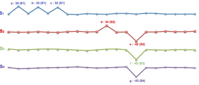
Example 2.1 (Hybrid Outlier). There are 4 time series s1, s2, s3, s4 in Figure 2.1, and a= 35, b = 33, c = 32, d= 34, e =−42, f =−42, g =−43 are time points in them. Time points d, e, f, gdramatically deviate from their neighbor time points, and they are self-trend outliers. Time points a, b, c, d are peer-wise outliers because of their great difference from the time points with the same timestamps in other time series. Our problem is to find hybrid outliers. d is a hybrid outlier, which is not only different from its neighbors, but also different from the time points with the same timestamps in other time series.

2.2 Detecting Outliers in Multiple Time Series

Given multiple time series, assuming that most of the time series are normal while a few are anomalous, the problem is to find all anomalous time series. In most of the methods for solving such problems, a model is first learned based on all the time series, and an outlier score for each time series is then computed with respect to the model. The model could be supervised or unsupervised, and we mainly review unsupervised models in this section.

(17)

2.2.1 Parametric Methods

A summary model is created on the base data in unsupervised parametric methods. For a test sequence, if the probability of generation of it from the model is super low, then the sequence is marked abnormal. The outlier score of the entire time series is computed based on the probability of each element. Markov chain models and Finite state automata (FSA) are two frequently used models.

Markov methods estimate the conditional probability for each symbol in a test sequence conditioned on the symbols preceding it. Most of the techniques utilize the short mem-ory property of sequences [33] and they store conditional information for a histmem-ory size k. Yeet al.[43] proposed a technique where a Markov model withk= 1 is used. A probabilistic suffix tree (PST) is a tree representation of a variable-order markov chain [36], which was used in [36] and [42] for efficient computations.

A fixed length Markovian technique (FSA) [25] determines the probability of a symbol, conditioned on a fixed number of preceding symbols, and the techniques were used for outlier detection in [11], [24], and [25]. The approach employed by FSA uses aFinite State Automaton to estimate the conditional probabilities [11]. FSA can be learned from length nsubsequences in training data. During testing, all lengthnsubsequences can be extracted from a test sequence and fed into the FSA. If the FSA reaches a state from where there is no outgoing edge corresponding to the last symbol of the current subsequence, then an anomaly is detected.

2.2.2 Discriminative Methods

Discriminative methods first define a distance function that measures the distance between two time series. Clustering algorithms are then applied to cluster time series, and the outlier score of a time series is computed as the distance to the centroid of the closest cluster. There are various distance measures and clustering algorithms.

The most straightforward distance measure for time series is the Euclidean Distance [16] and its variants, based on the commonLp -norms [44]. Dynamic time warping (DTW) was

introduced by Berndt et al. [6], which allows a time series to be stretched or compressed to provide a better match with another time series. Another group of distance measures for time series are developed based on the concept of the edit distance for strings. The best known such distance is the LCSS distance, utilizing the longest common subsequence

(18)

model [2], [39].

The majority of clustering algorithms can be applied on time series data, including k-Means [13], EM [28], phased k-k-Means [31], dynamic clustering [34], k-medoids [10], one-class SVM [15], etc. Since different clustering methods have different complexity, the selection of a clustering method depends on specific application domain.

The outliers identified by the methods reviewed in this section are entire time series, while our problem in this thesis is to detect hybrid outliers which are time points. Thus, those methods are obviously not suitable for solving our problem.

Example 2.2 (Outlier Time Series). Let us consider the same time series data in Exam-ple 2.1. The methods introduced in this section will find time series s1 as an outlier, which is different from the other time series.

To the best of our knowledge, we are the first to detect hybrid outliers on time series data.

(19)

Chapter 3

Problem Definition and Framework

In this chapter, we first present the formal definition of our problem in Section 3.1. Then, we propose a heuristic framework for detecting hybrid outliers in a time series database in Section 3.2.

3.1 Problem Definition

Definition 3.1(Time Data Point). A time data point (or time point for short) consists of a timestamp and an associated data value.

Definition 3.2(Time Series). A time seriessis a sequence of time points. The data values are ordered in timestamp ascending order. We assume that all timestamps take positive integer values. We denote by s[j]the time point of time seriess at timestamp j.

To keep our discussion simple, in this thesis, we assume that all time series are of the same length, denoted by m, i.e., each time series s has a time point s[j] at timestamp 1 ≤ j ≤ m. When the time series are not of the same length, alignments or dynamic warping can be applied as the preprocessing step. We also assume that all time series are normalized by Znormalization [18].

Example 3.1 (Time Point and Time Series). In Figure 3.1, s[1], s[2], s[3], s[4], s[5], s[6], and s[7] are time points. The value of time point s[3] is 1, and its timestamp is 3. s is a time series, and it is a sequence of those 7 time points.

(20)

CHAPTER 3. PROBLEM DEFINITION AND FRAMEWORK 10

Figure 3.1: An example of time series

Definition 3.3 (Segment). Given a time seriess of lengthm, s[j:e] =s[j]s[j+ 1]. . . s[e] (1 ≤ j ≤ e ≤ m) is the segment at timestamp interval [j : e]. The length of s[j : e] is

l=e−j+ 1.

When lis 1, i.e.,j=e, segments[j:e] is a time point.

Example 3.2 (Segment). In Figure 3.1, s[1 : 5] =s[1]s[2]s[3]s[4]s[5], s[2 : 6] =s[2]s[3]s[4] s[5]s[6], and s[3 : 7] =s[3]s[4]s[5]s[6]s[7] are three segments of length 5 in time series s.

In this thesis, among all time points in time series, what we are particularly interested in is outlier points.

Definition 3.4(Neighbor). Given a window sizew >0, for a time point s[j]in time series

s, a time point s[j0]is called a neighbor of s[j]if 0<|j−j0| ≤w.

Example 3.3 (Neighbor). When w= 2, time points s[2], s[3], s[5], and s[6] are neighbors of s[4] in Figure 3.1.

A self-trend outlier is a time point that deviates remarkably from its neighbors.

Definition 3.5 (Self-Trend Outlier). Suppose there is an outlyingness function Fs, which

measures the difference between a time point s[j]and its neighbors as the self-trend outlier degree sdeg[j] = Fs(s, j). Given a time series s and a self-trend outlier degree threshold

δs>0, a time point s[j]is a self-trend outlier if its self-trend outlier degree sdeg[j]≥δs.

Example 3.4 (Self-Trend Outlier). Assume we have a self-trend outlyingness function, which computes the smallest distance from a time point to its neighbors as the self-trend outlier degree. Supposeδs= 5 and the window size w is 2, for time series s in Figure 3.1,

(21)

Definition 3.6(Time Series Database). A time series database S consists ofntime series,

S={si|1≤i≤n}, where si is the i-th time series in S.

Definition 3.7(Peer). Given a time series databaseS, for a time pointsi[j]in time series

si, a time point si0[j]is called a peer of s_i[j]if i6=i0.

Example 3.5(Peer). In Figure 3.2, there is a time series database which consists of 7 time seriess1, s2,. . . ,s7, anda, b, c, . . . , i, j are time points in them. Time pointsd, h and iare peers of each other.

A peer-wise outlier is a time point whose behavior is exceptional comparing to its peers in a given set of time series.

Definition 3.8 (Peer-Wise Outlier). Suppose there is an outlyingness function Fp, which

measures the difference between a time point si[j]and its peers in a given set of time series

as the peer-wise outlier degree pdegi[j] =Fp(S, j, i). Given a time series si in a time series

databaseS and a peer-wise outlier degree threshold δp >0, a time point si[j]is a peer-wise

outlier if the peer-wise outlier degreepdegi[j]≥δp.

Example 3.6 (Peer-Wise Outlier). Assume we have a peer-wise outlyingness function, which computes the smallest distance from a time point to its peers in a given set of time series as the peer-wise outlier degree. Let us consider the time series database S in Fig-ure 3.2. Whenδp= 20, s1[5] is a peer-wise outlier, because the smallest distance from it to

the peers (s2[5], s3[5],s4[5]) is 35, which is greater thanδp, i.e., pdeg1[5] = 35> δp.

Self-trend outlier and peer-wise outlier are two different types of outliers, and they have different outlier behaviors. In practice, some outliers show their outlyingness in two ways. First, they may deviate greatly from their neighbors. Second, their behaviors may also be different from that of their peers. For example, in Figure 3.2, time pointj is different from its neighbors, and it also behaves differently from its peers. We call this type of outlier hybrid outlier. In general, a hybrid outlier has a combination of those two types of outlier behaviors.

Definition 3.9 (Hybrid Outlier Score). Hybrid outlier score (or outlier score for short)

oi[j]is a non-negative value which measures the hybrid outlier degree of a time point si[j].

Definition 3.10 (Hybrid Outlier). Suppose there is an outlyingness function F, which computes the expectation of a time pointsi[j] based on its neighbors and a set of its peers,

(22)

Figure 3.2: Small time series data

and gives the difference degree between si[j] and its expectation as the hybrid outlier score

oi[j] = F(S, j, i). Given a time series database S and a hybrid outlier threshold δ > 0, a

time pointsi[j] is called a hybrid outlier if the hybrid outlier score oi[j]≥δ.

Example 3.7 (Hybrid Outlier). Assume we have a hybrid outlyingness function, which computes the smallest distance from a time point to the peers in a given set of time series and its neighbors as the outlier degree. Suppose δ = 10 and w = 1. For the time series database in Figure 3.2, the smallest distance from time point s7[20] to the peers (s1[20],

s5[20]) and its neighbors (s7[19], s7[21]) is 16. Therefore, the outlier score o7[20] = 16> δ, ands7[20] is a hybrid outlier.

In this thesis, we tackle the problem of finding top N hybrid outliers in a time series database.

Problem Definition. Given a time series databaseS ={si|1≤i≤n}andN, where time

(23)

Table 3.1: The summary of symbols Symbol Description

S the time series database si thei-th time series in S

si[j] thej-th time point insi

n the number of time series in S

m the number of time points in a time series

si[j:e] the segment which starts at timestampj and ends at timestampe insi

l the length of a segment w the span of tracking window oi[j] the hybrid outlier score of si[j]

N the number of hybrid outliers to be detected

data is to find N hybrid outliers with the highest outlier scores. Table 3.1 summaries some frequently used symbols in this thesis.

3.2 Framework

In this section, a heuristic algorithm framework is proposed to detect hybrid outliers in a time series database. As discussed in Section 3.1, a hybrid outlier has a combination of self-trend outlier behavior and peer-wise outlier behavior. Heuristically, our framework iteratively compares each time point with the neighbors and a set of peers in the locally similar time series to compute the hybrid outlier score.

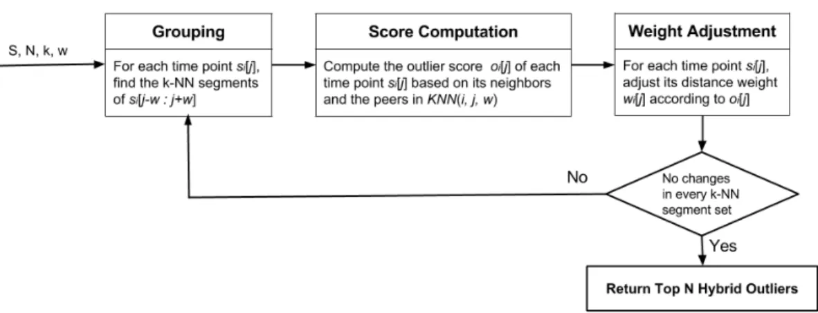
In Figure 3.3, we show an overview of our framework. Basically, to compute the outlier score of a time point si[j], our framework first finds out a set of segments S0={si0[j−w:

j+w]}, where si0[j−w:j+w] is similar tos_i[j−w:j+w] andi6=i0. We refer towas the

tracking window size. Then an intermediate outlier score ofsi[j] is calculated based on the

time points insi[j−w:j+w] and its peers inS0. After that, the distance between segments

will be adjusted andS0 will be updated accordingly. This process repeats untilS0 is stable, and the intermediate outlier score in the last iteration is returned as the final outlier score. To be specific, our framework mainly consists of three iterative phases: grouping phase, outlier score computation phase, and distance weight adjustment phase.

(24)

Figure 3.3: Overview of the framework

3.2.1 Grouping Phase

As discussed in Section 3.1, the hybrid outlier degree of a time point is affected by its self-trend outlier behavior and peer-wise outlier behavior. For a time pointsi[j], we compute

its outlier score based on its neighbor time points in si[j−w : j+w] and the peer time

points in a given set of time series. Because of that, we need to first find out a set of peers ofsi[j] whichsi[j] will be compared with. In this thesis, the k-Nearest Neighbors algorithm

(or k-NN for short) is applied to getksegmentssi0[j−w:j+w], denoted asKN N(i, j, w),

which are most similar to si[j −w : j+w] by distance, where i 6= i0. A general way to

calculate the k-NN distancedistknn(si[j :e], si0[j : e]) between two segments s_i[j : e] and

si0[j:e] is shown in Equation 3.1. distknn(si[j:e], si0[j:e]) = e X t=j (si[t]−si0[t])2 (3.1)

3.2.2 Score Computation Phase

After we get theKN N(i, j, w) of si[j−w:j+w] for time pointsi[j], its outlier score will

be computed based on its neighbors and the peers in KN N(i, j, w). Different algorithms which apply our framework can specify their own methods to calculate outlier scores. We will develop two such algorithms in Chapter 4 and the detailed methods of how to compute outlier scores will be discussed there.

(25)

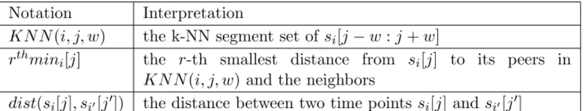
Table 3.2: Notations used in the algorithm framework Notation Interpretation

k the number of nearest neighbor segments of each si[j−w:

j+w]

wi[j] the distance weight of time point si[j]

KN N(i, j, w) the k-NN segment set of si[j−w:j+w]

KN N(i, j, w)∗ the k-NN segment set of si[j−w : j+w] in the previous

iteration ¯

o the average outlier score of all time points of all time series inS

topN O the hybrid outlier set with top N highest outlier scores

3.2.3 Distance Weight Adjustment Phase

An outlier scoreoi[j] is generated forsi[j] after the first two phases. One may use this score

as its final outlier score. However, since the peers inKN N(i, j, w) are only a subset of the peers ofsi[j], it may inaccurately gain a very high outlier score. For example, in Figure 3.2,

supposew= 4 and the 2-NN segments ofs2[10 : 18] ares3[10 : 18] ands4[10 : 18]. The time pointd(s2[14]) has a very high outlier score, because it is so different from its neighbors and the peers (s3[14], s4[14]). However, s2[10 : 18] is also similar to s5[10 : 18] ands6[10 : 18], and d(s2[14]) is not supposed to have a very high outlier score because of its similarity to h(s5[14]) andi(s6[14]).

To get more accurate outlier scores, the k-NN distance between segments will be adjusted iteratively based on the outlier scores. In this way, a time point would have a chance to be compared with its peers in different k-NN segments during the iterations. To achieve that, we assign a distance weightwi[j] to each time point si[j] when calculating the k-NN

distance between segments. The formal definition ofwi[j] is as follows.

Definition 3.11(Distance Weight). Given a time series databaseS and a time pointsi[j],

the distance weight wi[j]of si[j] is defined as

wi[j] =

¯ o oi[j]

,

where oi[j] is the outlier score of si[j], and o¯is the average outlier score of all time points

of all time series in S, i.e.,

¯ o= n P i m P j oi[j] mn .

(26)

The higher outlier score oi[j] is, the less distance weight wi[j] is. Ifoi[j] is more than ¯o,

the distance between two points would be shrunk; otherwise, the distance would be enlarged.

Definition 3.12 (Segment k-NN Distance). Given two segments si[j :e]and si0[j :e], the

k-NN distance betweensi[j :e] andsi0[j:e]is defined as

distknn(si[j:e], si0[j:e]) = e

X

t=j

(wi[t]wi0[t](s_i[t]−s_i0[t]))2.

The length of k-NN segment is 2w+ 1. The window size w affects the similarity of two segmentssi[j−w:j+w] andsi0[j−w:j+w] for each time points_i[j]. Withwincreasing,

the similarity will be determined by more time points in si and si0, and s_i[j−w :j+w]

will have more globally similar trends with the k-NN segments,i.e., the time pointsi[j] will

be compared with the peers in the more globally similar time series. When w decreases, si[j−w:j+w] and the k-NN segments are more locally similar.

The three phases of our framework, i.e., grouping phase, outlier score computation phase, and distance weight adjustment phase, will repeat until everyKN N(i, j, w) is equal toKN N(i, j, w)∗, where KN N(i, j, w)∗ is the k-NN segment set of si[j−w:j+w] in the

previous iteration.

Algorithm 1 shows the pseudo code of the framework for detecting hybrid outliers in a time series database. Table 3.2 lists the symbols used in the framework for ease of presen-tation. Algorithm 1 iteratively computes the k-NN segments according to Definition 3.12, calculates outlier scores of all time points in all time series based on the difference from them to their neighbors and a set of their peers, and adjusts distance weight for every time point using Definition 3.11. The outlier score of each time point may change with the new k-NN in each iteration, and the outlier score in each iteration is the minimal one so far. Finally topN hybrid outliers can be identified according to their outlier scores.

Example 3.8 (Algorithm Framework). A time series database S which consists of 7 time series s1, s2,. . . , s7 is shown in Figure 3.2. Suppose k = 2, N = 1 and w = 4, we detect the top 1 hybrid outlier inS.

We first get the initial 2-NN segments ofsi[j−w:j+w]for each si[j]by segment k-NN

distances, as shown in the second column of Table 3.3. Then an intermediate outlier score of each time pointsi[j]is calculated as the second smallest distance from it to its neighbors and

(27)

Algorithm 1:Hybrid Outlier Detection Algorithm Framework

Input: S;N;k;w.

Output: topN O

1 Normalize each s_i ∈S if necessary byZNormalization; 2 foreachsi ∈ S do 3 foreach si[j]∈ si do 4 w_i[j]←1; 5 Initialize KN N(i, j, w) and KN N(i, j, w)∗; 6 do 7 foreach si ∈ S do 8 foreach s_i[j]∈ s_i do 9 KN N(i, j, w)∗ ←KN N(i, j, w);

10 Compute KN N(i, j, w) based on Definition 3.12; 11 foreach si ∈ S do 12 foreach si[j]∈ si do 13 Compute o_i[j]; 14 Calculate ¯o; 15 foreach s_i ∈ S do 16 foreach si[j]∈ si do 17 Calculate wi[j] by Definition 3.11; 18 while anyKN N(i, j, w)6=KN N(i, j, w)∗; 19 Compute topN O based on the final outlier scores; 20 return topN O;

in s2[10 : 18] except for itself and the time points (s3[14], s4[14]). Since d deviates greatly from those time points, it has a very high outlier score in this iteration. The second row of Table 3.4 shows the rank of time points ordered by their outlier scores in the first iteration, where d is the top 1 outlier. When the first iteration is done, the distance weight of each time point will be calculated according to the intermediate outlier score by Definition 3.11. Sincedhas the highest outlier score, its distance weight will be the smallest.

In the second iteration, with the change of distance weight, the k-NN distance between segments is adjusted by Definition 3.12, and each 2-NN segment set is updated accordingly as shown in the third column of Table 3.3. The outlier score of each time point is then recalculated based on its neighbors and the peers in the new 2-NN segments. The third row of Table 3.4 shows the rank of time points ordered by their outlier scores in the second iteration. Interestingly, the 2-NN segments ofs2[10 : 18] for time point d(s2[14]) change to be s5[10 : 18] and s6[10 : 18], and its outlier score goes down due to its similarity to h and

(28)

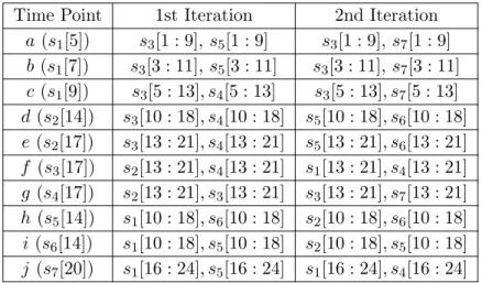
Table 3.3: 2-NN segments during iterations Time Point 1st Iteration 2nd Iteration

a(s1[5]) s3[1 : 9],s5[1 : 9] s3[1 : 9],s7[1 : 9] b(s1[7]) s3[3 : 11],s5[3 : 11] s3[3 : 11], s7[3 : 11] c(s1[9]) s3[5 : 13], s4[5 : 13] s3[5 : 13], s7[5 : 13] d(s2[14]) s3[10 : 18], s4[10 : 18] s5[10 : 18], s6[10 : 18] e(s2[17]) s3[13 : 21], s4[13 : 21] s5[13 : 21], s6[13 : 21] f (s3[17]) s2[13 : 21], s4[13 : 21] s1[13 : 21], s4[13 : 21] g (s4[17]) s2[13 : 21], s3[13 : 21] s3[13 : 21], s7[13 : 21] h (s5[14]) s1[10 : 18], s6[10 : 18] s2[10 : 18], s6[10 : 18] i(s6[14]) s1[10 : 18], s5[10 : 18] s2[10 : 18], s5[10 : 18] j (s7[20]) s1[16 : 24], s5[16 : 24] s1[16 : 24], s4[16 : 24] Table 3.4: The outlier degree rank of time points during iterations

Rank 1 2 3 4 5 6 7 8 9 10

1st Iteration d h i j a c b f e g

2nd Iteration j a c b h i d f e g

i. After the second iteration, the algorithm terminates because there are no more changes in 2-NNs, and j is returned as the top 1 hybrid outlier.

The algorithms for detecting hybrid outliers in a time series database can apply this framework by specifying the outlier score calculation methods. To show the feasibility of our framework, two algorithms based on the framework are developed in Chapter 4.

3.2.4 Convergence

Since our framework is iterative, it is necessary to discuss its property of convergence.

Lemma 3.1. Let KN Nt=

KN N(1,1, w), . . . , KN N(1, m, w), KN N(2,1, w), . . . , KN N(2, m, w), . . . , KN N(n,1, w), . . . , KN N(n, m, w) be the vector of k-NN segment sets for all time points in the t-th iteration. Ot=

o1[1], . . . , o1[m], o2[1], . . . , o2[m], . . . , on[1], . . . , on[m]

denotes the vector of outlier scores for all time points in the t-th iteration. If p < q andKN Np =KN Nq, then Oq =Oq−1.

Proof. We prove the lemma by contradiction. AssumeOq6=Oq−1whenp < qandKN Np =

(29)

there must exist a time pointsi[j] whose outlier scoreoi[j]qin theq-th iteration is not equal

to the outlier score oi[j](q−1) in the (q−1)-th iteration, i.e., oi[j]q 6= oi[j](q−1). Because

the outlier score in each iteration is the minimal one so far and p ≤ (q −1), we can get oi[j]p ≥ oi[j](q−1). Since KN Np = KN Nq, i.e., the KNN segment set for time point si[j]

in thep-th iteration is the same as that in theq-th iteration, o0_i[j]q=o0_i[j]p ≥oi[j]p, where

o0_i[j]t_{is the intermediate outlier score computed according to the peers in}_{KN N}₍_{i, j, w}_{) and}

the neighbors in the t-th iteration. Sinceoi[j]q =min(o0_i[j]q, oi[j](q−1)), o0_i[j]q ≥oi[j]p, and

oi[j]p ≥oi[j](q−1), we can getoi[j]q =oi[j](q−1), which is a contradiction.

Lemma 3.2. If Oq=Oq−1, then the framework will terminate in the (q+ 1)-th iteration. Proof. By definition, we have

distknn(si[j:e], si0[j:e]) = e X t=j (wi[t]wi0[t](s_i[t]−s_i0[t]))2, wi[j] = ¯ o oi[j] , ¯ o= n P i m P j oi[j] mn . Using the above three equations, we have

distknn(si[j:e], si0[j:e]) = e X t=j ( n P i m P j oi[j])2 m2_n2_o i[t]oi0[t](si[t] −si0[t]) !2 .

Since Oq =Oq−1,i.e.,oi[j]q=oi[j](q−1), everyKN N(i, j, w) in the (q+ 1)-th iteration

will be the same as that in theq-th iteration based on the above equation. Our framework will terminate in the (q + 1)-th iteration according to the termination condition of the framework.

Lemma 3.3. Given a time series databaseSwhich consists ofntime series of lengthm, and let KN Nt=

KN N(1,1, w), . . . , KN N(1, m, w), KN N(2,1, w), . . . , KN N(2, m, w), . . . , KN N(n,1, w), . . . , KN N(n, m, w)

be the vector of k-NN segment sets for all time points in the t-th iteration, the possible number of distinctKN Nt is(Cnk−1)mn.

(30)

Proof. There are C_nk₋₁ possible different k-NN segment sets KN N(i, j, w) for each time point si[j]. Since there are m×n time points in total, the possible number of distinct

KN Nt is (Cnk−1)mn.

Theorem 3.1. After at most (C_nk₋₁)mn+ 2iterations, our framework terminates.

Proof. According to Lemma 3.3, there must exist two iterationspandq such thatKN Np =

KN Nq and 1 ≤ p < q <= (Cnk−1)mn+ 1. Then, by Lemma 3.1, we can get Oq = Oq−1. In this way, the framework will terminate in the (q+ 1)-th iteration by Lemma 3.2. Since q+ 1≤(C_nk₋₁)mn+ 2, our framework terminates after at most (C_nk₋₁)mn+ 2 iterations.

Corollary 3.1. Since m, n, k are finite, the upper bound on the number of iterations (C_nk−1)mn+ 2 is finite. As a result, the framework must converge in a finite number of iterations.

(31)

Chapter 4

Two Algorithms

In Section 3.2 we propose a heuristic framework to detect hybrid outliers. In this chapter, two algorithms based on the framework are developed by specifying outlier score compu-tation methods. The implemencompu-tation of those two algorithms verifies the feasibility of our framework.

In Section 4.1, a distance-based algorithm which calculates outlier scores according to distances between time points is presented. We also propose a prediction-based algorithm using the deviation of the actual value of a time point from its predicted value as the outlier score in Section 4.2. In Section 4.3, we use a small data example to further describe our two algorithms.

4.1 The Distance-based Algorithm (DA)

Basically, to get the outlier score of a time pointsi[j], the distance-based algorithm (or DA

for short) calculates the distances fromsi[j] to the following time points.

• The neighbors of si[j], i.e., the time points insi[j−w:j+w] except forsi[j] itself.

• The peers of si[j] inKN N(i, j, w).

In the DA algorithm, the distance between two time points is the absolute value of their difference, which is defined as:

dist(si[j], si0[j0]) =|s_i[j]−s_i0[j0]|. (4.1)

We formally define the hybrid outlier score in the DA algorithm as follows.

(32)

CHAPTER 4. TWO ALGORITHMS 22

Table 4.1: Notations used in the distance-based algorithm Notation Interpretation

KN N(i, j, w) the k-NN segment set of si[j−w:j+w]

rthmini[j] the r-th smallest distance from si[j] to its peers in

KN N(i, j, w) and the neighbors

dist(si[j], si0[j0]) the distance between two time pointss_i[j] and s_i0[j0]

Table 4.2: Three time series

1 2 3 4 5 6

s1 11 12 12 19 11 12 s2 12 11 10 11 10 12 s3 13 11 11 12 11 13

Definition 4.1(Hybrid Outlier Score in the DA Algorithm). Given a time series database

S, a time point si[j], the k-NN segments KN N(i, j, w), and a parameter 1 ≤r ≤ 2w+k,

the outlier scoreoi[j] of si[j]in DA is defined as

oi[j] =rthmini[j],

where rth_min

i[j] is the r-th smallest distance from si[j] to its peers in KN N(i, j, w) and

the neighbors insi [23] [30] [5] [27] [7].

The outlier score computation method in DA is shown in Algorithm 2, and Table 4.1 lists the symbols used in the DA algorithm.

Example 4.1(Outlier Score Computation in DA). In Table 4.2, there are three time series. Suppose k = 2, w = 1, r = 2, and KN N(1,4,1) = {s2[3 : 5], s3[3 : 5]}, we compute the outlier score o1[4] of time point s1[4].

First we calculate the distances froms1[4] to its neighbors (s1[3], s1[5]) by Equation 4.1, dist(s1[4], s1[3]) =|19−12|= 7,

dist(s1[4], s1[5]) =|19−11|= 8.

Then, the distances froms1[4] to the peers (s2[4],s3[4]) are calculated, dist(s1[4], s2[4]) =|19−11|= 8,

(33)

Algorithm 2:Outlier Score Calculation Method in DA

Input: si[j];si;KN N(i, j, w); w;r.

Output: oi[j]

1 rthmin_i[j]←+∞;

2 foreachsi[j0]∈ si do

3 if 1≤ |j−j0| ≤wthen

4 Compute dist(s_i[j], s_i[j0]) by Equation 4.1; 5 if dist(s_i[j], s_i[j0])< rthmin_i[j]then 6 Update rthmin_i[j];

7 8

9 foreachs_i0[j−w, j+w]∈ KN N(i, j, w) do

10 Compute dist(si[j], si0[j]) by Equation 4.1;

11 if dist(si[j], si0[j])< rthmin_i[j]then

12 Updaterthmini[j];

13

14 oi[j]←rthmini[j];

15 return o_i[j];

dist(s1[4], s3[4]) =|19−12|= 7.

Thus, the 2nd smallest distance from s1[4] to its peers in KN N(1,4,1) and the neighbors is2thmin1[4] = 7, i.e., o1[4] = 7.

4.2 The Prediction-based Algorithm (PA)

The prediction-based algorithm (or PA for short) predicts the value of a time point si[j]

by applying the least squares technique for multi-variate linear regression [29], and computes the deviation of the actual valuesi[j] from its predicted valuesi[j]∗ as its outlier

score. Table 4.3 gives a list of notations used in this section.

For a time point si[j] withw < j ≤m−w, wherew is a parameter that we refer to as

the tracking window size andm is the length of time series si, the PA algorithm estimates

its value by using two sources of information.

• The neighbors of si[j], i.e.,si[j−w], . . . ,si[j−1], si[j+ 1], . . . , si[j+w].

(34)

Table 4.3: Notations used in the prediction-based algorithm Notation Interpretation

si[j]∗ the predicted value of time pointsi[j]

KN N(i, j, w) the k-NN segment set ofsi[j−w:j+w]

v the number of independent variables in multi-variate regres-sion

Ai the optimal regression coefficient matrix of time seriessi

Xi the matrix of independent variables forsi, each row is sample

values of the corresponding independent variables Yi the column vector of desired values forsi

For a time point si[j] with j ≤ w, its value is estimated based on the time points in

si[1 : 2w+ 1] except for si[j] itself and its peers inKN N(i, w+ 1, w); for a time pointsi[j]

withj > m−w, we predict its value according to the time points insi[m−2w:m] except

forsi[j] and the peers inKN N(i, m−w, w).

To be specific, we try to predict the value ofsi[j] as a linear combination of its neighbor

time points and the peer time points in KN N(i, j, w) = {si1[j−w, j +w], si2[j−w, j +

w], ..., sik[j−w, j+w]}. Mathematically, we have the following equation forw < j≤m−w:

si[j]∗ = a1si[j−1] +a2si[j−2] +· · ·+awsi[j−w]+

aw+1si[j+ 1] +aw+2si[j+ 2] +· · ·+a2wsi[j+w]+

a2w+1si1[j] +a2w+2si2[j] +· · ·+a2w+ksik[j]

(4.2)

Equation 4.2 is a collection of linear equations for j = w+ 1, . . . , m−w, with si[j] being

the dependent variable, si[j−1], . . . , si[j−w], si[j+ 1], . . . , si[j+w], si1[j], si2[j], . . . ,

sik[j] the independent variables. The number of independent variables is

v= 2w+k. (4.3)

Each ax is called a regression coefficient. The least square solution, i.e., regression

coeffi-cients which minimize the sum of squares errors SSE=

m

X

j=1

(si[j]−si[j]∗)2,

is given by the multi-variate regression [14]. With this set up, the optimal regression coef-ficientsAi for time series si are given by [8]

(35)

Algorithm 3:Outlier Score Calculation Method in PA

Input: si[j];si;KN N(i, j, w); w. Output: oi[j] 1 if j= 1 then 2 SetXi; 3 SetYi; 4 Calculate A_i by Equation 4.4; 5 Calculate s_i[j]∗ by Equation 4.5; 6 o_i[j]← |s_i[j]−s_i[j]∗|; 7 return oi[j];

where Xi is an m × v matrix, the j-th row of the matrix Xi consists of sample values of

the corresponding independent variable forsi[j] in Equation 4.2. Yi is a column vector of

actual valuessi[j], i.e.,Yi is anm ×1 matrix. Ai is av ×1 matrix.

Thus,si[j]∗ is computed based on Equation 4.2 as follows.

si[j]∗ = v

X

c=1

Xi[j][c]Ai[c]. (4.5)

Definition 4.2 (Hybrid Outlier Score in the PA Algorithm). For a time point si[j], the

outlier score oi[j]of si[j]in PA is defined as

oi[j] =|si[j]−si[j]∗|,

where si[j]∗ is the predicted value of si[j].

The method for computing outlier scores in the PA algorithm is presented in Algorithm 3. For all time points in time series si, we only need to calculate Ai once, i.e., it is only

calculated when we compute the predicted value ofsi[1]. The detailed computation of the

outlier score of a time point is shown in Example 4.2.

Example 4.2 (Outlier Score Computation in PA). Let us consider the same time series as in Example 4.1, and we compute the outlier score o1[4] of time point s1[4]. The span of tracking window sizewis 1, and the 2-NN segments of eachs1[j−1, j+ 1]ares2[j−1, j+ 1] ands3[j−1, j+ 1].

Since w = 1 and k = 2, the number of independent variables for each time point is v = 2×1 + 2 = 4 by Equation 4.3. First, the matrix X1 is set, each row of X1 consists of

(36)

the sample values of the corresponding independent variable for each time point in s1. For example, the independent variables fors1[4] are in the 4-th row of X1, where X1 is

X1 =              12 12 12 13 11 12 11 11 12 19 10 11 12 11 11 12 19 12 10 11 19 11 12 13              .

The matrixY1 is also set, which actually is a column vector of real values of time points in s1, shown as following: Y1 =              11 12 12 19 11 12              .

Then we compute the optimal regression coefficientsA1 by Equation 4.4 and get

A1 =         −0.27 −0.02 −1.21 2.55         .

Finally, based on A1 and the 4-th row of X1, the predicted value of s1[4] is s1[4]∗= 12·(−0.27) + 11·(−0.02) + 11·(−1.21) + 12·(2.55) = 13.83 by Equation 4.5. Therefore, the outlier score of s1[4] is o1[4] =|19−13.83|= 5.17.

4.3 Example

A time series database which consists of 7 time series s1, s2,. . . , s7 is shown in Figure 3.2. Each time series has 24 time points, where a = 35, b = 33, c = 32, d = 34, e = −42, f =

(37)

Table 4.4: 2-NN segments during iterations for DA Time Point 1st Iteration 2nd Iteration a(s1[5]) s3[1 : 9],s5[1 : 9] s3[1 : 9],s7[1 : 9] b(s1[7]) s3[3 : 11],s5[3 : 11] s3[3 : 11], s7[3 : 11] c(s1[9]) s3[5 : 13], s4[5 : 13] s3[5 : 13], s7[5 : 13] d(s2[14]) s3[10 : 18], s4[10 : 18] s5[10 : 18], s6[10 : 18] e(s2[17]) s3[13 : 21], s4[13 : 21] s5[13 : 21], s6[13 : 21] f (s3[17]) s2[13 : 21], s4[13 : 21] s1[13 : 21], s4[13 : 21] g (s4[17]) s2[13 : 21], s3[13 : 21] s3[13 : 21], s7[13 : 21] h (s5[14]) s1[10 : 18], s6[10 : 18] s2[10 : 18], s6[10 : 18] i(s6[14]) s1[10 : 18], s5[10 : 18] s2[10 : 18], s5[10 : 18] j (s7[20]) s1[16 : 24], s5[16 : 24] s1[16 : 24], s4[16 : 24] Table 4.5: Outlier score of each time point during iterations for DA

Time Point a b c d e f g h i j

1st Iteration 3 2 3 33 1 1 1 33 30 17

2nd Iteration 3 2 3 1 1 1 1 1 1 17

−42, g = −43, h = 35, i = 34, j = 20 are 10 time points among the 168 time points. We apply the DA and PA algorithms to iteratively compute the outlier scores of the time points, and the results are presented in Subsection 4.3.1 and Subsection 4.3.2, respectively.

4.3.1 The DA Result

Setk= 2, r = 2, and w= 4. Initially, the outlier score oi[j] of each time pointsi[j] is set

to infinity and the distance weight wi[j] is 1. We compute KN N(i, j,4), oi[j], and wi[j]

iteratively.

• The 1st iteration

After calculating the k-NN distances between segments by Definition 3.12, we get the Table 4.6: Distance weight of each time point during iterations for DA

1st Iteration 0.43 0.65 0.43 0.04 1.29 1.29 1.29 0.04 0.04 0.08 2nd Iteration 0.20 0.31 0.20 0.62 0.62 0.62 0.62 0.62 0.62 0.04

(38)

Table 4.7: Final outlier degree rank of time points for DA

Rank 1 2 3 4 5 6 7 8 9 10

Time Point j a c b h i d f e g

Table 4.8: 2-NN segments during iterations for PA

Time Point 1st Iteration 2nd Iteration 3rd Iteration a(s1[5]) s3[2 : 8],s5[2 : 8] s5[2 : 8],s6[2 : 8] s5[2 : 8],s6[2 : 8] b(s1[7]) s3[4 : 10],s5[4 : 10] s5[4 : 10],s6[4 : 10] s5[4 : 10], s6[4 : 10] c(s1[9]) s3[6 : 12], s5[6 : 12] s2[6 : 12], s6[6 : 12] s2[6 : 12], s6[6 : 12] d(s2[14]) s3[11 : 17], s4[11 : 17] s4[11 : 17], s5[11 : 17] s5[11 : 17], s6[11 : 17] e(s2[17]) s3[14 : 20], s4[14 : 20] s1[14 : 20], s6[14 : 20] s1[14 : 20], s6[14 : 20] f (s3[17]) s2[14 : 20], s4[14 : 20] s2[14 : 20], s4[14 : 20] s2[14 : 20], s4[14 : 20] g (s4[17]) s2[14 : 20], s3[14 : 20] s2[14 : 20], s3[14 : 20] s2[14 : 20], s3[14 : 20] h (s5[14]) s1[11 : 17], s6[11 : 17] s1[11 : 17], s6[11 : 17] s2[11 : 17], s6[11 : 17] i(s6[14]) s1[11 : 17], s5[11 : 17] s2[11 : 17], s5[11 : 17] s2[11 : 17], s5[11 : 17] j (s7[20]) s1[17 : 23], s5[17 : 23] s5[17 : 23], s6[17 : 23] s5[17 : 23], s6[17 : 23]

2-NN segments of si[j−w :j+w] for each si[j], as shown in the second column of

Table 4.4. The second row of Table 4.5 demonstrates the outlier scores of a, b, . . . , j calculated based on the distances from each time point to its peers inKN N(i, j,4) and the neighbors. For instance, the outlier score of a(s1[5]) is the 2nd smallest distance from it to the time points in s1[1 : 9] except for itself and the time points (s3[5],s5[5]), i.e.,o1[5] = 3. The average outlier score of all time points of all time series is 1.29 in this iteration. Then the distance weight is adjusted by Definition 3.11, as shown in the second row of Table 4.6.

• The 2nd iteration

Table 4.9: Outlier scores of time points during iterations for PA

1st Iteration 0.05 0.02 0.03 3.74 0.3 0.03 0.01 0.14 0.03 9.88 2nd Iteration 0.05 0.02 0.03 0.25 0.3 0.03 0.01 0.14 0.02 8.33 3rd Iteration 0.05 0.02 0.03 0.075 0.3 0.03 0.01 0.01 0.02 8.33

(39)

Table 4.10: Distance weight of time points during iterations for PA

1st Iteration 9.2 23 15.33 0.12 1.53 15.33 46 3.29 15.33 0.05 2nd Iteration 7.8 19.5 13 1.56 1.3 13 39 2.79 19.5 0.05

3rd Iteration 7.2 18 12 4.8 1.2 12 36 36 18 0.04

Table 4.11: Average score of all time point in all time series during iterations for PA 1st Iteration 2nd Iteration 3rd Iteration

¯

o 0.46 0.39 0.36

According to the distance weight of time points in the first iteration, the 2-NN seg-ments are updated, shown in the third column of Table 4.4. The outlier score of each time point is then recalculated based on its neighbors and the peers in the new 2-NN segments, as shown in the third row of Table 4.5. The third row of Table 4.6 shows the recalculated distance weight. In addition, the average outlier score is 0.62. After two iterations, there are no more changes in all 2-NN segment sets, and the outlier scores in the 2nd iteration are returned as the final outlier scores. Table 4.7 shows the final rank of time points ordered by their outlier scores in the DA algorithm. From the final result, we can see that our algorithm indeed finds out the outlier pointj which is not only different from its neighbors, but also different from the peers.

The result also shows how our algorithm can get more accurate outlier scores by adjusting distance weight in each iteration. For example, in the first iteration, the 2-NN segments of s2[10 : 18] ares3[10 : 18] ands4[10 : 18]. Time pointd(s2[14]) gets a very high outlier score, because ddeviates remarkably from the time points in s2[10 : 18] except for itself and the peers (s3[14], s4[14]). However, after the distance weight adjustment, the 2-NN segments become s5[10 : 18] and s6[10 : 18] in the second iteration, and the outlier score of ddrops because it is similar to the time pointsh (s5[14]) andi (s6[14]).

4.3.2 The PA Result

Setk= 2, w= 3. Similar to the DA algorithm, we compute KN N(i, j,3), oi[j], and wi[j]

iteratively in the PA algorithm. There are 3 iterations for PA. The results ofKN N(i, j,3), oi[j],wi[j], and ¯oduring iterations are shown in Tables 4.8, 4.9, 4.10, and 4.11, respectively.

¯

(40)

Table 4.12: Final outlier degree rank of time points for PA

Rank 1 2 3 4 5 6 7 8 9 10

Time Point j e d a c f b i g h

outlier degree rank of time points in our PA algorithm. The outlier pointj is also identified by our PA algorithm.

(41)

Chapter 5

Experiments

To validate the effectiveness and efficiency of our two algorithms named DA and PA, we conducted experiments on a real data set and a series of synthetic data sets. The experi-mental results on a real currency exchange rate data set are reported in Section 5.1, and we present the results on synthetic data sets in Section 5.2.

All methods were implemented in Java and all experiments were conducted on a PC computer with an Intel Core i5-2400 3.10GHz CPU and 4GB main memory running 64-bit CentOS 6.5.

We cannot identify any existing method that solves the exact same problem. The focus of our methods is to find hybrid outliers on time series data. Consequently, this thesis does not intend to compete with the existing methods.

5.1 Results on a Real Data Set

We obtained an exchange rate data set from the Pacific Exchange Rate Service of University of British Columbia1_{. The data set consists of monthly exchange rates of 62 currencies w.r.t.} USD from 1974 to 2013. We normalized the data set by Znormalization [18].

As a case study, Figure 5.2 shows 7 currency time series in 2009-2013, and they are CAD, EUR, GBP, JPY, HKD, CHF, and RUB. A time point is denoted as the currency name concatenating its timestamp. For instance, the exchange rate of CAD in January 2009 is denoted as CAD2009.01. We setk= 2, w = 6, andr = 2 for DA, and k= 2 and w= 6

1

http://fx.sauder.ubc.ca/

(42)

CHAPTER 5. EXPERIMENTS 32

Table 5.1: Top 10 hybrid outliers detected by our two algorithms

DA PA CHF2011.08 RUB2009.02 GBP2009.05 GBP2013.03 JPY2013.01 CHF2011.08 EUR2009.02 HKD2012.02 GBP2013.12 EUR2009.02 CHF2011.07 HKD2011.11 RUB2009.03 JPY2009.01 RUB2009.02 GBP2013.09 GBP2009.03 GBP2013.12 EUR2009.11 JPY2012.03

Table 5.2: Top 10 hybrid outliers detected by the baselines DA Baseline PA Baseline CHF2011.08 CHF2011.08 GBP2009.05 RUB2009.02 JPY2013.01 CHF2011.09 EUR2009.02 GBP2013.03 GBP2013.12 HKD2011.03 CHF2011.07 HKD2012.02 RUB2009.03 HKD2010.12 RUB2009.02 HKD2011.10 GBP2009.03 EUR2010.10 RUB2012.06 GBP2011.08

for PA. The top 10 outliers in the 7 time series detected by our two algorithms are shown in Table 5.1. By observation those time points are indeed not only different from their neighbors, but also different from the peers. CHF2011.08 has a very high hybrid outlier score for both algorithms. It is a locally highest point of CHF time series, while other series have downward trends at the same time. Interestingly, we found a news article2 about the strength of CHF during summer 2011. According to another article3, the rise of CHF was caused by the European debt crisis, and investors increasingly sought secure investments in

2

http://money.cnn.com/2011/08/31/markets/swiss_franc/index.htm

(43)

Table 5.3: Top 10 self-trend and peer-wise outliers Self-trend Peer-wise GBP2009.05 HKD2011.08 RUB2009.02 HKD2011.07 CHF2011.08 HKD2011.03 HKD2010.06 HKD2011.06 EUR2010.05 HKD2011.09 RUB2009.04 JPY2013.12 CHF2011.07 HKD2011.02 HKD2010.11 JPY2013.09 HKD2010.05 JPY2013.11 GBP2010.05 JPY2013.10

Switzerland that is considered a safe haven, during times of crisis.

As the baseline methods, we compute k-NN segments without distance weight assign-ment for each time point, and use the outlier scores in the first iteration as the final outlier scores. The top 10 hybrid outliers found by the baseline methods are shown in Table 5.2. The results of the PA baseline contain four top 10 hybrid outliers identified by PA. For the results of the DA baseline, RUB2012.06 is the only time point which is not in the top 10 hybrid outliers detected by DA. This is because RUB2012.06 is compared with its peers in different k-NN segments during the iterations in our DA algorithm. The 2-NN segments for RUB2012.06 are the segments of time series GBP and CHF in the first iteration of DA. However, since time series RUB is also similar to time series EUR during 2012, the 2-NN segments change to be the segments of time series EUR and GBP, and the outlier score of RUB2012.06 drops in the second iteration. Therefore, our algorithms can get more accurate outlier scores comparing to the baselines.

Table 5.3 shows the top 10 self-trend outliers and peer-wise outliers in the 7 currency time series. Ther-th smallest distance from each time point to its neighbors is computed as the self-trend outlier degree, and we compute ther-th smallest distance from each time point to the peers as the peer-wise outlier degree, where w= 6, k = 2 and r = 2. Interestingly, we observe that time series EUR, GBP, and HKD are similar to each other from January 2010 to December 2010. Because of that, even though GBP2010.05, EUR2010.05, and HKD2010.05 are top 10 self-trend outliers, their hybrid outlier scores are not high. On the other hand, JPY2013.09, JPY2013.10, JPY2013.11 and JPY2013.12 are peer-wise outliers,

(44)

however, they are neighbors and similar to each other, so they are also not in the final top 10 hybrid outliers.

We also test the scalability of our two algorithms by using random samples of various sizes of the exchange rate data set. Figures 5.1(a) and 5.1(b) show the scalability of the two algorithms with respect to 2 different factors, the numbernof time series, and the number m of time points in each time series. The two algorithms are scalable as the size of data set grows. Figures 5.1(c) and 5.1(b) investigate the number of iterations of the algorithms when n and m vary, respectively, on the real data set. The number of iterations increases slowly withn and m increasing. DA converges faster than PA, which explains the reason why DA runs faster than PA to some extent.

(a) m = 480 (b) n = 62

(c) m = 480 (d) n = 62

(45)

Table 5.4: The description of 4 real data sets

Name Description n m

Temperature the monthly temperature of 48 states of the USA in 1994-2013

48 240 Exchange Rate the monthly exchange rate of 20 currencies w.r.t.

USD in 1999-2013

20 180 Interest Rate the monthly interest rate of 26 countries in

2001-2011

26 130 Government GDP the yearly real government net capital stock as a

percentage of real GDP of 22 countries in 1960-2001

22 42

5.2 Results on Synthetic Data Sets

We insert outliers into 4 real data sets to generate synthetic data sets. The real data sets are temperature data set4, exchange rate data set5, interest rate data set6, and government GDP data set7. The description of the 4 real data sets is in Table 5.4, wherenis the number of time series andm is the number of time points in each time series. The outlier injection process contains following two steps.

• Step 1: Given a time series database S, randomly select x time series from S.

• Step 2: For each selected time series si in step 1, replace the value of time points

si[j] with an extreme value forj =fi, fi+y, fi+ 2y, fi+ 3y, . . . , fi+bm−_yficy, where

0< y < mis a parameter andfiis a random value between 0 toy. Theextreme value

in our context is defined in Definition 5.1.

Definition 5.1(Extreme Value). Given a time seriessi, an interquartile range [3] of time

point samples insi is

IQR=Q3−Q1,

where Q3 is the third quartile [3] and Q1 is the first quartile [3] of si. An extreme value V

4 ftp://ftp.ncdc.noaa.gov/pub/data/ghcn/v3/ 5_{http://fx.sauder.ubc.ca/data.html} 6 http://www.economicswebinstitute.org/data/eurointerest-longterm.xls 7 http://www.economicswebinstitute.org/data/EU_all%20data%20for%20is-lm.zip

(46)

Table 5.5: Original time series

1 2 3 4 5 6 7 8 9 10 11 12 13

s1 11 9 13 10 14 12 8 7 13 15 12 11 10 s2 12 11 10 11 10 12 10 11 9 8 13 10 11 s3 13 11 11 12 11 13 12 13 10 8 9 10 9

Table 5.6: Synthetic time series

1 2 3 4 5 6 7 8 9 10 11 12 13

s1 11 9 19 10 14 12 8 7 2 15 12 11 10 s2 12 11 10 11 10 12 10 11 9 8 13 10 11 s3 13 11 11 12 11 13 12 13 10 8 9 10 9

is a random value in the range of[Vmin1, Vmin2]or [Vmax1, Vmax2], where Vmin1 =Q1−2C·IQR,

Vmin2 =Q1−C·IQR, Vmax1 =Q3+C·IQR, Vmax2=Q3+ 2C·IQR, andC >1 is a parameter. C is 1.5 by default.

Example 5.1 (Outlier Injection). In Table 5.5, there is a time series database S which consists of 3 time series. Suppose x = 1 and y = 6, we inject outliers into S. We first randomly selectx= 1 time series to be injected outliers fromS, and s1 is selected. We then replace the values of time pointss1[3] and s1[3 + 6] with extreme valuesV for f1= 3. Since Q1 = 10, Q3 = 13 and IQR = 3 for s1, V is a random value in the range of [1,5.5] or [17.5,22] by Definition 5.1. The time series data injected outliers are shown in Table 5.5, and the values of s1[3] ands1[9] are 19 and 2, respectively.

We conduct experiments to test the effectiveness and efficiency of our two algorithms regarding the following parameters.

• x - the number of time series selected to be injected outliers;

(47)

• k - the number of nearest neighbor segments of eachsi[j−w:j+w];

• w - the span of tracking window.

x and y are parameters for generating synthetic data sets, andk and w are parameters of our hybrid outlier detection algorithms.

Our two algorithms named DA and PA are applied to the synthetic data sets to detect top N hybrid outliers, and N is set to be the number of injected outliers for each data set. We use the variable controlling method to conduct our experiments. In each variable controlled test, we compare the performance of DA with that of PA.

5.2.1 Effectiveness

Therecallin our context is defined in Definition 5.2. Figures 5.3(a), 5.4(a), 5.5(a), and 5.6(a) show the recall of the two algorithms whenxvaries for the 4 synthetic data sets. In general, we can achieve a recall ranging from 0.6 to 0.99, and the recall is over 0.8 on the synthetic temperature data set when y = 40, k = 4, and w = 5. The recall first increases and then decreases with x increasing for 4 synthetic data sets. Figures 5.3(b), 5.4(b), 5.5(b), and 5.6(b) provide an illustration of the trend of recall when y changes. The recall first increases and then decreases, and our two algorithms have very similar trends.

Definition 5.2 (Recall of a Method). Suppose there are doutliers injected in the original data set, and the injected outlier set is denoted as Od. Given a method A that returns top

N (N =d) hybrid outlier set, denoted bytopN O, the recall of methodA,recallA, is defined

as

recallA=

|Od∩topN O|

d ,

where |Od∩topN O| is the number of elements in intersection ofOd and topN O.

Besides the parameters for generating synthetic data sets, we also examine how the recall changes with respect to the parameters of our two algorithms. By default, r = 5 for DA. The results on the change of k are shown in Figures 5.3(c), 5.4(c), 5.5(c), and 5.6(c). In general, our two algorithms can achieve a recall ranging from 0.7 to 0.99. In most cases, the recall drops with k increasing for the two algorithms. The results with respect to the span of tracking windoww are shown in Figures 5.3(d), 5.4(d), 5.5(d), and 5.6(d). Similar to k, when w increases, the recall decreases gradually. We also test the recall of the DA

(48)

algorithm with respect tor on the 4 synthetic data sets. The recall first increases and then decreases whenr increases, which is shown in Figure 5.7.

In summary, DA outperforms PA in terms of recall in most cases, and PA is more sensitive to parameter selection compared to DA.

5.2.2 Efficiency

We also test the efficiency of our two algorithms. Figures 5.3(e), 5.4(e), 5.5(e), 5.6(e) and Figures 5.3(f), 5.4(f), 5.5(f), 5.6(f) show the running time in logarithmic scale of our two algorithms with k and w varying, respectively, on the 4 synthetic data sets. The running time of DA and PA both increases whenk and w increase. DA runs faster than PA in all cases.

5.3 Summary of Results

We conduct experiments to test the effectiveness and efficiency of our two algorithms. There are 3 parameters that can affect the performance of DA, and the performance of PA can be affected by 2 parameters. We test our algorithms by varying one parameter in each test and compare their performance.

Generally speaking, in terms of recall, DA performs better than PA. Our two algorithms can achieve a recall ranging from 0.7 to 0.99 in most cases. For the efficiency, DA runs faster than PA, and PA converges slower than DA. DA and PA are both scalable as the size of data set grows.

(49)

(50)

(a) y = 40, k = 4, w = 5 (b) x = 5, k = 4, w = 5

(c) x = 3, y = 80, w = 5 (d) x = 3, y = 80, k = 4

(e) x = 3, y = 80, w = 5 (f) x = 3, y = 80, k = 4

(51)

(a) y = 20, k = 4, w = 5 (b) x = 4, k = 4, w = 5

(c) x = 5, y = 80, w = 5 (d) x = 5, y = 80, k = 6

(e) x = 5, y = 80, w = 5 (f) x = 5, y = 80, k = 6