Département des Sciences Économiques
de l'Université catholique de Louvain
Efficient Importance Sampling
for ML Estimation of SCD Models
L. Bauwens and F. Galli
CORE DISCUSSION PAPER 2007/53
EFFICIENT IMPORTANCE SAMPLING FOR ML ESTIMATION OF SCD MODELS
Luc Bauwens1 and Fausto Galli2
August 17, 2007
Abstract
The evaluation of the likelihood function of the stochastic conditional duration model requires to compute an integral that has the dimension of the sample size. We apply the efficient importance sampling method for computing this integral. We compare EIS-based ML estimation with QML estimation based on the Kalman filter. We find that EIS-ML estimation is more precise statistically, at a cost of an acceptable loss of quickness of computations. We illustrate this with simulated and real data. We show also that the EIS-ML method is easy to apply to extensions of the SCD model.
Keywords: stochastic conditional duration, importance sampling.
JEL Classification: C13, C15, C41
1
CORE and Department of Economics, Universit´e catholique de Louvain.
2
Swiss Finance Institute at University of Lugano
Bauwens’s work was supported by a FSR grant from UCL. He is also a member of ECORE, a newly created association between ECARES and CORE.
This text presents research results of the Belgian Program on Interuniversity Poles of Attraction initiated by the Belgian State, Prime Minister’s Office, Science Policy Programming. The scientific responsibility is
1
Introduction
The stochastic conditional duration (SCD) model is a dynamic duration model that was
proposed by Bauwens and Veredas (2004) as an alternative to the autoregressive conditional
duration model of Engle and Russell (1998). These models are typically applied to analyze
the dynamics of the intra-daily trading activity of financial markets. The SCD model uses
two unobservable stochastic components for one observable variable (the duration), implying
that one of the stochastic terms must be integrated over the whole sample to compute the
likelihood function. The fact that the variables to be integrated enter the model nonlinearly
leads to the necessity to compute this high-dimensional integral by simulation. The same
problem arises for the stochastic volatility (SV) model, since it has the same structure as the
SCD model.
The solution proposed by Bauwens and Veredas in their original paper circumvented the
integration problem since they used quasi-maximum likelihood (QML) estimation based on an
approximation of the model by a linear space state representation. This makes it possible to
use the Kalman filter to approximate the likelihood function. This method has the advantage
of being simple and fast in terms of numerical computation and of providing consistent and
asymptotically normal estimators (under suitable regularity conditions), but it is in principle
suboptimal in finite samples.
To avoid approximations, in the literature on SV models other estimation procedures have
been proposed, for instance the generalized method of moments (GMM), the efficient method
of moments (EMM), and Bayesian estimation based on Markov chain Monte Carlo (MCMC)
sampling. For a survey of these procedures see E. Ghysels and Renault (1996). Some of
these methods have been extended to the estimation of SCD models. Ning (2004) proposes to
estimate SCD models via the empirical characteristic function (ECF) and GMM. Maximum
likelihood estimation based on MCMC integration of the latent variables is instead adopted
by Feng, Jiang, and Song (2004) to estimate a SCD model in the form proposed by Bauwens
and Veredas (2004) and an extended version with a leverage effect determined by the presence
and Martin (2006) in the context of Bayesian estimation.
A relatively new method for computing the integral needed for evaluating the likelihood
function of models with latent variables relies on the efficient importance sampling (EIS)
procedure, recently developed by Richard and Zhang (1998). This method consists in an
extension of the well known importance sampling technique and seems to be particularly well
suited for the computation of the multidimensional though relatively well behaved integral
needed for evaluation the SCD likelihood. An application to an extended family of SV models
is provided in Liesenfeld and Richard (2003) who illustrate the flexibility of this algorithm.
The purpose of this article is to extend to the original SCD model of Bauwens and Veredas
(2004) the EIS method of numerical sampling, to compare it to the QML estimation method
on simulated and real data, and to use it in order to analyze some extensions of the original
specification proposed by Bauwens and Veredas. Our main finding is that for the order of
magnitude of the sample sizes used in practice, i.e. a few thousands, there is a substantial
efficiency gain in favour of EIS-ML.
The article is organized in the following way. In section 2 we present the main features of
the SCD model which are necessary to the subsequent analysis. In Section 3 we detail the EIS
numerical integration method employed for ML estimation of the SCD model. In section 4
we apply this method to several simulated data sets and compare the sampling distributions
of EIS-ML and QML estimates. In section 5 the EIS-ML technique is applied to the same
dataset used in Bauwens and Veredas (2004) and a comparison is drawn. Two examples of
parametric extensions of the SCD model which are easily estimated by EIS-ML are provided
in Section 6. The last section contains our concluding remarks.
2
SCD models: main features
In this section, we present briefly the SCD model. A more detailed description can be found
in Bauwens and Veredas (2004). If we denote by xi the duration between two events that
happened at times ti−1 and ti, and assume that the stochastic process {xi} generating the
model can be written as
xi =eψii (1)
with
ψi =ω+βψi−1+ui, (2)
where |β|<1 to ensure the stationarity of the process, and
ui∼iidN(0, σ2), (3)
i ∼iid p(i), (4)
with p(.) a distribution with positive support, anduj independent ofi,∀i, j.
The moments and autocorrelation function of this process are
E(xi) =µe ω 1−β+ 1 2 σ2 1−β2 1 +δx2= (1 +δ2)e σ2 1−β2 ρk= e σ2βk 1−β2−1 (1+δ2) (e σ2 1−β2−1) ≈ σ2βk/(1−β2) (1+δ2) (e σ2 1−β2−1) ≈βρk−1, (5)
where µ stands for E(i), δx for the dispersion index (i.e. the standard deviation to mean
ratio) ofxi, andδfor the dispersion index ofi. The autocorrelation functionρkgeometrically
decreases at rateβ only asymptotically with respect tok, while for smallkthe decrease rate is smaller.
Given a sequencexofnrealizations of the process, with densityg(x|ψ, θ1) indexed by the
parameter vectorθ1, conditional on a vectorψ of latent variables of the same dimension asx,
and given the densityh(ψ|θ2) indexed by the parameter θ2, the likelihood function of x can
be written as:
L(θ;x) =L(θ1, θ2;x) =
Z
g(x|ψ, θ1)h(ψ|θ2)dψ. (6)
assumptions we made, it can be sequentially decomposed as f(x, ψ|θ1, θ2) = n Y i=1 p(xi|ψi, θ1)q(ψi|ψi−1, θ2), (7)
where p(xi|ψi, θ1) is obtained fromp(i) using the change of variable in (1) (so thatθ1
corre-sponds to the parameters ofp(.)), andq(ψi|ψi−1, θ2) is the Gaussian densityN(ω+βψi−1, σ2)
(so thatθ2includesω,βandσ2). Given the functional form usually adopted forp(i) (Weibull,
gamma, generalized gamma...), the multidimensional integral in (6) cannot be solved
analyt-ically and must be computed numeranalyt-ically by simulation.
To perform a QML estimation, one can use the following transformation of the model:
lnxi =η+ψi+ξi,
ψi =ω+βψi−1+ui,
where ξi = lni −η and η = E(lni). This puts the model in state space form with zero
mean errors. The ensuing distribution of ξi can be approximated by a Gaussian one, and the
Kalman filter applied to compute the approximate likelihood.
3
EIS based ML estimation
Alternative approaches to QML inference for the SCD model can be based on Monte Carlo
methods. These methods are widely used in Bayesian inference to evaluate moments of
high-dimensional posterior densities when they are not known analytically. One reason for their
success is the relative ease with which they can be applied. EIS, in particular, allows a very
accurate evaluation of the likelihood function and has been shown to be quite reliable for
the estimation of SV models and of latent factor intensity models, see Bauwens and Hautsch
(2006). Another advantage of this algorithm is that its basic structure does not depend on
a specific model. This renders changes in the distributional assumptions for the underlying
random variables rather simple.
(1998). In this section, we present the basics of its motivation and functioning and we detail
its implementation in the context of the ML estimation of SCD models.
Assume one has to evaluate a unidimensional functional integral of the form
G(y) =
Z
Λ
g(y, λ)p(λ)dλ, (8)
wheregis a integrable function with respect to a density p(λ) with support Λ. The vectory
denotes an observed data vector, which in our context corresponds to the observed durations.
A Monte Carlo (MC) estimate of (8) is
¯ GS(y) = 1 S S X i=1 g(y,λ˜i), (9)
where the ˜λi’s are draws from p and S is the number of draws. In cases where one cannot
generate directly draws fromp(λ), one can resort to importance sampling (IS). The IS prin-ciple consists of replacing the initial sampler p(λ) with an auxiliary parametric importance samplerm(λ, a), which is an easy-to-simulate density forλ, indexed by the parameter vector
a. To apply importance sampling, equation (8) is transformed into
G(y) =
Z
Λ
g(y, λ) p(λ)
m(λ, a)m(λ, a)dλ, (10) and the corresponding IS-MC estimate of G(y) is
¯ GS,m(y, a) = 1 S S X i=1 g(y,˜λi) p(˜λi) m(˜λi, a) , (11)
where the ˜λi’s now denote draws from the IS densitym.
The aim of efficient importance sampling (EIS) is to minimize the MC variance of the
estimator in (11) by selecting optimally the parameters aof the importance function density
Given independent draws ˜λi’s, the sampling variance of ¯GS,m(y, a) is given by Var( ¯GS,m(y, a)) =G(y)V(a, y), (12) where V(a, y) = 1 G(y) Z Λ g(y, λ)p(λ) m(λ, a) −G(y) 2 m(λ, a)dλ. (13) If we denote byk(λ, a) the density kernel of the IS samplerm(λ, a) and byχ(a) its integral, such thatm(y, a) = kχ(λ,a(a)),V(a, y) in (13) can be rewritten as
V(a, y) = Z Λ h(d2(y, a, λ))g(y, λ)p(λ)dλ, (14) where d(y, a, λ) = lng(y, λ)−lnp(λ)−lnk(λ, a)−lnG(y)−lnχ(a), (15) and h(c) =e √ c+e−√c−2 = 2 ∞ X i=1 ci (2i)!. (16)
Noting that the termd(y, a, λ) is supposed to be small if an efficient sampler is used, the function h(c) can be approximated by its leading term c to get
V(a, y)≈V˜(a, y) =
Z
Λ
d2(y, a, λ)g(y, λ)p(λ)dλ. (17)
Minimizing the MC variance amounts then to minimizing the quadratic termd2(y, a, λ). It can be shown that if the importance samplermbelongs to the exponential family, the problem remarkably simplifies to a least squares minimization problem for the components of the vector
of auxiliary parametersa.
Extending the EIS approach to the case where λ is of high dimension, like in the SCD model (whereλcorresponds to theψ vector), requires that we can decompose the minimiza-tion problem in a series of unidimensional subproblems.
given by ˜ L(θ;x) = 1 S S X j=1 " n Y i=1 p(xi|ψ˜(ij), θ1) # , (18)
where ˜ψi(j) denotes a draw from the densityq(ψi|ψi−1, θ2). This approach bases itself only on
the information provided by the distributional assumptions of the model and does not consider
the information that comes from the observed sample. It turns out that this estimator is highly
inefficient since its sampling variance rapidly increases with the sample size. In any practical
case of a duration data set, where the sample sizenlies between 500 and 50000 observations, the Monte Carlo sampling sizeSrequired to give precise enough estimates ofL(θ;x) would be too high to be affordable and it turns out that this estimator cannot be relied on practically.
EIS tries to make use of the information provided by the observed data in order to come to
a reasonably fast and reliable numerical approximation. Let{m(ψi|ψi−1, ai)}ni=1be a sequence
of auxiliary samplers indexed by the set of auxiliary parameter vectors{ai}ni=1. These densities
can be defined as a parametric extension of the natural samplers {q(ψi|ψi−1, θ2)}ni=1. We
rewrite the likelihood function as
L(θ;x) = Z " n Y i=1 f(xi, ψi|xi−1, ψi−1, θ) m(ψi|ψi−1, ai) n Y i=1 m(ψi|ψi−1, ai) # . (19)
Then, its corresponding IS-MC estimator (the equivalent of (11)) is given by
˜ L(θ;x, a) = 1 S S X j=1 " n Y i=1 f(xi,ψ˜i(j)(ai)|xi−1,ψ˜i(−j)1(ai−1)) m( ˜ψi(j)(ai)|ψ˜i(−j)1(ai−1), ai) # . (20)
where{( ˜ψi(j)(ai)}ni=1 are trajectories drawn from the auxiliary samplers.
Relying on the factorized expression of the likelihood, the MC variance minimization
problem can be decomposed in a sequence of subproblems for each elementiof the sequence of observations, provided that the elements depending on the lagged valuesψi−1 are transferred
product of a function ofψi and ψi−1 and one of ψi−1 only, such that m(ψi|ψi−1, ai) = k(ψi, ai) χ(ψi−1, ai) = R k(ψi, ai) k(ψi, ai)dψi , (21)
we can set up the following minimization problem:
ˆ ai(θ) = arg min ai M X j=1 {ln h f(xi,ψ˜i(j)|ψ˜i(−j)1, xi−1, θ)χ( ˜ψ (j) i ,ˆai+1) i −ci−ln(k( ˜ψi(j), ai)}2, (22)
where ci is constant that must be estimated along with ai. If the density kernel k(ψi, ai)
belongs to the exponential family of distributions, the problem becomes linear in ai, and
this greatly improves the speed of the algorithm, as a least squares formula can be employed
instead of an iterative routine.
The estimated ˆai are then substituted in (20) to obtain the EIS estimate of the likelihood.
The EIS algorithm can be initialized by direct sampling, as in equation (18), to obtain a first
series of ˜ψi
(j)
and then iterated to allow the convergence of the sequences of {ai}, which is
usually obtained after 3 to 5 iterations. EIS-ML estimates are finally obtained by maximizing ˜
L(θ;x, a) with respect toθ.
If we adopt a Weibull distribution for i with parameterγ (=θ1) and a N(0, σ2) one for
ui, we come up with the following expressions:
p(xi|ψi−1, γ) = γ eψi−1 xi eψi−1 γ−1 expn− xi eψi−1 γo , (23) q(ψi|ψi−1, θ2) = 1 σ√2π exp − 1 2σ2(ψi−ω−βψi−1) 2 . (24)
A convenient choice for the auxiliary sampler m(ψi, ai) is a parametric extension of the
natural sampler q(ψi|ψi−1, θ2), in order to obtain a good approximation of the integrand
without too heavy a cost in terms of analytical complexity. Following Liesenfeld and Richard
(2003), we can start by the following specification of the functionk(ψi, ai):
whereζ(ψi, ai) =exp{a1,iψi+a2,iψi2}andai = (a1,ia2,i). This specification is rather
straight-forward and has two advantages. Firstly, asq(ψi|ψi−1, θ2) is present in a multiplicative form,
it cancels out in the objective function in (22), which becomes a least squares problem with
lnζ(ψi, ai) that serves to approximate lnp(xi|ψi−1, θ1) + lnχ(ψi−1, ai). Secondly, such a
func-tional form for k leads to a distribution of the auxiliary sampler m(ψi, ai) that remains
Gaussian, as stated in the following theorem, whose proof is given in the appendix.
Theorem 1 If the functional forms for q(ψi|ψi−1, θ2) and k(ψi, ai) are as in equations (24)
and (25) respectively, then the auxiliary density m(ψi|ψi−1, ai) = χk(ψ(ψi−i,a1,ai)i) is Gaussian, with
conditional mean and variance given by:
µi =vi2( ω+βψi−1 σ2 +a1,i), vi2= 1−2σσ22a 2,i, (26)
and the functionχ(ψi−1, ai) is given by
1 p 1−2σ2a 2,i exp ( σ2 2(1−2σ2a 2,i) ω+βψi−1 σ2 +a1,i 2 − 1 2 ω+βψi−1 σ 2) (27)
By applying these results, it is possible to compute the likelihood function of the SCD
model for a given value ofθ, based upon the following steps:
Step 1. Use the natural sampler q(ψi|ψi−1, θ2) to draw S trajectories of the latent variable
n
˜
ψi(j)
on
i=1, as in (18).
Step 2. The draws obtained in step 1 are used to solve for eachi(in the order fromnto 1) the least squares problems described in (22), which takes the form of the auxiliary linear
regression: lnγ−γψ˜i(j)+ (γ−1) lnxi− xi eψ˜ (j) i γ + lnχ( ˜ψi(j),ˆai+1) = a0,i+a1,iψ˜(ij)+a2,i( ˜ψ(ij))2+ε(ii), j= 1, ..., S,
where ε(ii) is the error term, a0,i is a constant term, and χ( ˜ψ(ij),ˆai+1) is set equal to 1
fori=nand defined by (27) for i < n.
Step 3. Use the estimated auxiliary parameters ˆai to obtain S trajectories
n
˜
ψi(j)(ˆai)
oN
i=1 from
the auxiliary sampler m(ψi|ψi−1,ˆai), applying the result of theorem 1.
Step 4. Return to step 2, this time using the draws obtained with the auxiliary sampler. Steps
2, 3 and 4 are usually iterated a small number of times (from 3 to 5), until a reasonable
convergence of the parameters ˆai is obtained.
Once the auxiliary trajectories have attained a reasonable degree of convergence, the simulated
samples can be plugged in formula (20) to obtain an EIS estimate of the likelihood. This
procedure is embedded in a numerical maximization algorithm that converges to a maximum
of the likelihood function. After convergence, we compute the standard errors from the
Hessian matrix.
4
Simulation results
In order to assess the gain in performance allowed by EIS-ML estimation in comparison with
QML, we conducted several repeated simulation experiments with different parameter
con-figurations. As the QML estimator should be consistent but inefficient in relatively small
samples, trajectories of 250, 500, 1000, 5000 and 10000 observations form a SCD data
gener-ating process (DGP) were simulated 1000 times and the model was estimated both by EIS-ML
and by QML. The idea to use as much as 10000 observations comes from the wish to judge
the loss of efficiency of QML relative to EIS-ML. Moreover, such sample sizes are far from
unusual for real data sets of durations.
The estimations were performed using the MaxSQPF constrained maximization function
of Ox console 3.40, under Windows XP with a dual core Intel 2.0 Gb processor. The speed
of estimation varies from a few seconds for a series of 250 data to a few minutes for a 10000
data one. EIS -ML estimation is much slower, with a computing time ranging from 10 to 100
and we suspect that alternative estimation strategies, such as Bayesian MCMC, would be
even slower than EIS-ML, as the results of Bauwens and Rombouts (2004) for the SV model
clearly show.
The DGP is defined by equations (1)-(4), plus formula (23). The parameter values used
in the simulations of the DGP were the following:
• ω = 0.0,
• β = 0.9,
• σ = 0.05 and 0.2,
• γ = 0.8 and 1.1,
thus leading to four combinations. The starting values for likelihood optimizations were set
for all estimations toω = 0.0, β = 0.85, σ = 0.15 and γ = 1.05, but we checked that other reasonable starting values provided quite similar results to those discussed below.
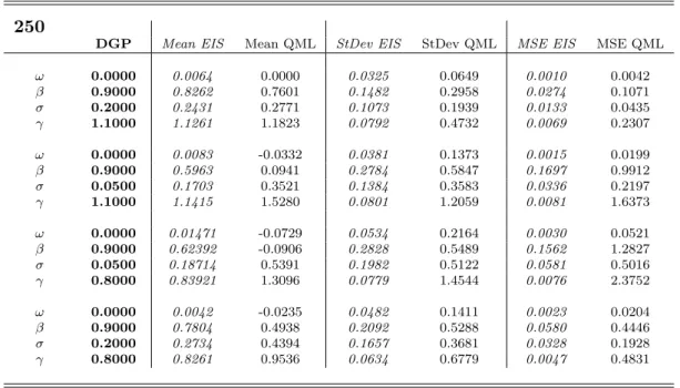
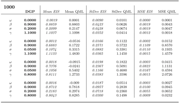
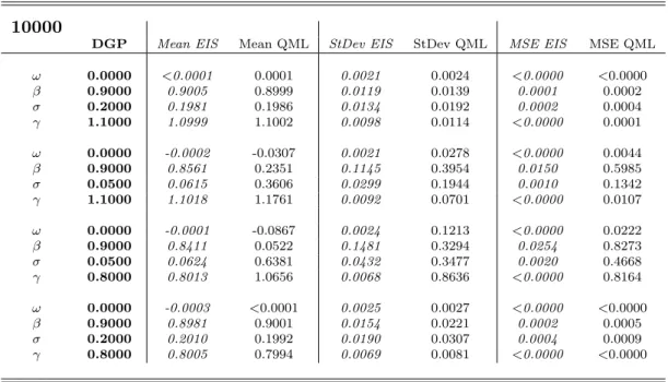
Tables 1 to 5 contain the means, standard deviations and mean-squared errors of the
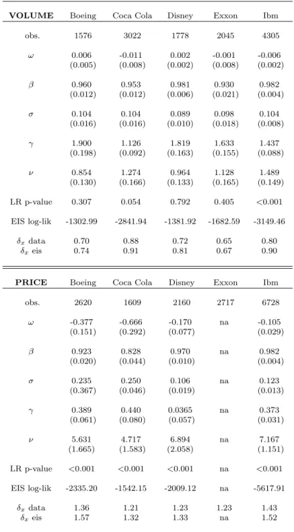
1000 estimates for each experiment, and figures 1 to 4 display the corresponding sampling
densities (obtained by kernel based smoothing). As a first remark, it can be noticed that in
both estimation methods there is a tendency to underestimate the autoregressive parameter
β and to overestimate the parameter σ, especially when the latter takes the low value of 0.05. Anyway, also in these cases the EIS-ML method provides estimates which in mean are
closer to the DGP parameters than the QML one. The most striking result concerns the
efficiency of the estimators: the EIS-ML estimated standard deviations of the estimates are
always remarkably smaller than the QML ones, in particular when the parameterσ is equal to 0.05. The combination of smaller bias and variance is reflected clearly in the mean-squared
errors, which are sensibly lower across the board for the EIS-ML method. The better general
performance of the EIS-ML estimator can be appreciated also by a visual inspection of the
sampling densities.
Looking at the tables and at figures 2 and 3 it is easy to remark how poor the performance
shows for each parameter the graph of the estimated standard deviations against the value
ofσ in the DGP, for a sample size of 1000. These results are based on additional simulations (for values of σ ranging from 0.02 to 0.7). This figure shows that for small values of σ in the DGP, both estimation methods tend to be imprecise. This is understandable, since as
σ tends to 0, the parameter β becomes unidentified, so that the likelihood function becomes flat. We also see in figures 2 and 3 that for the sampling distribution of the estimates of β
have a mode at (or close to) zero. However, the problem of is far more pronounced for QML
than for EIS-ML.
In order to dispel the doubt that the QML estimator might not be consistent (or that
the computer program is poorly written) we present in table 6 the results based on ten
QML estimations with one million data. From all this evidence we conclude that when the
sample size is not very large (of the order of hundreds of thousands), QML estimation can be
extremely inefficient if the standard deviation of second error term is small.
5
Estimation results for real data
In this section, we apply EIS-ML estimation to some data sets used by Bauwens and Veredas
(2004) for QML estimation, and we compare the results. The SCD model is exactly the same
as in the previous section, and as in these authors’ article.
The considered data sets correspond to five stocks traded at the New Your Stock Exchange
(NYSE): Boeing, Coca Cola, Disney, Exxon and Ibm (the last one was not used by Bauwens
and Veredas). The data were extracted from the trades and quotes database (TAQ) of the
NYSE and are relative to the months of September, October and November, 1996. From
the original trade and quote durations, price and volume duration were computed. Price
durations measure the amount of time before observing a given cumulated variation (up or
down) of the price (in this case, $1/8). Analogously, volume durations measure the amount
of time necessary to observe a cumulative traded volume of a given amount (25000 shares).
As it is customary in the literature on financial durations, the durations have been purged
the strong seasonality featured, both on a daily and a weekly basis, by key characteristics of
the duration processes. Price and volume durations feature a strong intra-day effect, being
smaller at the start and at the end of the trading day than around lunch time. Moreover, this
effect may depend on the day of the week. These deterministic time-of-day and day-of-the
week effect are controlled by nonparametrically regressing the observed durations of each day
of the week on the time of the day, and by defining the deseasonalized durations as the original
ones divided by the fitted values of the regression.
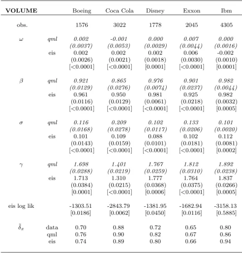
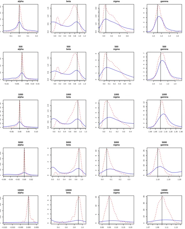
In tables 7 and 8 we present the estimated parameters of the QML and EIS-ML
estima-tions. For volume duration, even if the values taken by the estimates of the parameters for
the two methods considered are substantially the same, it is noticeable that the standard
errors of EIS-QML are generally lower, sometimes substantially, than the QML ones. We
also report in the table the computed dispersion index (˜δx) of the durations implied by the
estimates. This is computed by plugging in formula (5) the point estimates. We see that
the data dispersion index is better approximated if we estimate with the EIS-ML algorithm.
The estimates and standard errors for the price duration data are more markedly different
between the two methods than for volume durations. Moreover, the improved match between
the data dispersion index and the implied one of the EIS-ML estimates is even more striking
in this case. To draw a conclusion, provided that the model is correctly specified, by using
EIS-ML estimation rather than QML, the estimates one gets are more precise.
Finally, in both table, in square brackets, we present the MC standard deviations of the
EIS estimates. These standard deviations are calculated from ten different different estimates
obtained by running the algorithm using each time a different random seed for the common
random numbers employed in the EIS evaluation of the likelihood. The resulting dispersion
of the estimates is extremely low, which suggests that EIS is a rather robust method in this
6
Extensions
In order to illustrate the flexibility of EIS-ML as a numerical tool, we estimate two extensions
of the the SCD model described and used in the previous sections. The first extension consists
in the introduction of a “leverage” term in the mean of the latent factor. For a motivation
of this effect, we refer the reader to Feng, Jiang, and Song (2004), but we slightly differ from
these authors by letting the value ofψi to depend on the lagged durationxi−1 (rather than
i−1), such that equation (2) becomes
ψi=ω+βψi−1+αxi−1+ui. (28)
The introduction of the lagged observed duration requires just a slight modification of the
code and the effect on the speed of the algorithm is negligible: the EIS based computation
of the likelihood takes almost exactly the same time while of course the introduction of an
extra parameter slows down the maximization routine. Table 9 presents the results of the
estimation with the data sets employed in the previous section. The introduction of the
lagged duration as an explanatory variable can be tested by the likelihood ratio for the null
hypothesisα = 0. The p-values are reported in the table in curled brackets before the value of the likelihood at its maximum.
For volume durations, the estimated leverage coefficients do not display a clear sign
pat-tern. Moreover, the results of the LR tests are mixed: we clearly reject the null only for
Exxon, with a positive leverage effect, while in three other cases the evidence is mixed
(p-value around 0.05) and the effect is negative. In the case of Boeing, the leverage effect is
clearly not significant. For price durations the results are clearly in favor of a negative
lever-age effect, except for the puzzling case of the Exxon stock, where the estimates are somewhat
unusual (lowβ and highσ).
In the second variant of the model we change the distribution of variablei, representing
the baseline duration. The Weibull distribution is replaced by a generalized gamma one with
parameters (ν, γ, c). The third parameter is a location parameter and, like in the case of the Weibull, it is chosen so that the random variable has a unitary mean (so thatcis a function of
ν and γ and therefore does not appear in the parameters to estimate). The density function of the generalized gamma is as follows:
fGG() = γ cνγΓ(ν) νγ−1exph− c γi , (29)
and it can be easily seen that the Weibull density is a particular case, arising when ν = 1. Further information about this distribution is available in Bauwens and Giot (2001), who
provide a detailed description of its characteristics.
The modifications in the computer code that were required to use this extension were
even simpler than in the case of the leverage effect. We did not observe any speed impact
on the likelihood computation, while, of course, its maximization was a tad slower because
of the introduction of an extra parameter. The estimation results are available in table 10.
Volume durations modeling does not appear to improve consistently with the introduction
of this richer baseline density. The p-values of the LR tests for the null hypothesis ν = 1 are seldom low (except for Ibm) as the values taken by the parameter ν tend to be rather close to 1. Different results are obtained with price durations. A significant departure from
the Weibull is observed (estimates of ν are between 4.7 to 7.2) and gains in likelihood are consistent, to the point that the p-values of the LR tests for ν = 1 are always smaller than 0.001. For the price durations of the Exxon stock the EIS-ML algorithm delivers a value for
the likelihood but the maximization routine failed to achieve strong convergence, regardless
of the vector of initial parameters chosen as a starting point.
7
Conclusion
This paper describes a new approach, the EIS-ML, for the numerical estimation of SCD
models, showing its capability to deliver more precise estimates than the approximate QML
method. The performance EIS-ML are tested both in a simulated and a real case, giving good
results in terms of precision of estimation at a cost of an acceptable loss in rapidity of the
computation. The evidence from the estimation of simulated series suggests an uncomfortably
appears to be much more robust. The algorithm is applied to the estimation of a set of
volume and price durations showing a remarkably low MC variance. Moreover, we observed
a significant gain in the capability of the SCD model in reproducing the first two empirical
moments of the data when QML is replaced by EIS-ML estimation. Further interesting
extensions are explored in the use of EIS-ML for the estimation of richer specifications, such as
the presence of a leverage effect in the autoregressive component or a more flexible distribution
for the baseline duration.
Appendix
Proof: [Theorem 1]Given (24) and the definition ofζ(ψi, ai) following (25), the function k(ψi, ai) is given by
k(ψi, ai) =q(ψi|ψi−1, ai)ζ(ψi, ai) = 1 σ√2πexp ( −1 2 h 1 σ2 −2a2,i ψi2−2 ω+βψi−1 σ2 +a1,i ψi + ω+βψi−1 σ 2 i ) . (30)
Integratingk(ψi, ai) with respect toψi, we obtain the functionχ(ψi−1, ai) given in (27). If we
combine (30) and (27) as in (21), we find the functional form of m(ψi|ψi−1, ai), that can be
in (26): m(ψi|ψi−1, ai) =k(ψi, ai)/χ(ψi−1, ai) = p 1−2σ2a 2,i σ√2π exp ( −1 2 h 1 σ2 −2a2,iψ 2 i −2 ω+βψi−1 σ2 −a1,i ψi + σ 2 1−2σ2a 2,i ω+βψi−1 σ2 +a1,i 2 i ) = 1 vi √ 2π exp −1 2 1 vi2ψ 2 i −2 µi v2iψi+ µ2 i vi2 = 1 vi √ 2π exp − 1 2v2 i (ψi−µi)2 . (31)
References
Bauwens, L.,andP. Giot(2001): Econometric modelling of stock market intraday activity.
Kluwer Academic Publishers.
Bauwens, L.,and N. Hautsch (2006): “Stochastic conditional intensity processes,”
Jour-nal of Financial Econometrics, 4, 450–493.
Bauwens, L., and J. Rombouts (2004): “Econometrics,” in Handbook of Computational
Statistics, ed. by J. Gentle, W. Hrdle,and Y. Mori, vol. 1. Springer Verlag.
Bauwens, L., and D. Veredas (2004): “The stochastic conditional duration model: a
latent factor model for the analysis of financial durations,”Journal of Econometrics, 119(2),
381–412.
C. Strickland, C. F., and G. Martin(2006): “Bayesian analysis of the stochastic con-ditional duration model,” Computational Statistics and Data Analysis, 50(9), 2247–2267.
E. Ghysels, A. H.,andE. Renault(1996): “Stochastic volatility,” inHandbook of
Engle, R.,andJ. R. Russell(1998): “Autoregessive conditional duration: a new approach
foor irregularly spaced transaction data,” Econometrica, 66, 1127–1162.
Feng, D., G. Jiang, and P. Song (2004): “Stochastic conditional duration models
with leverage effect for financial transaction data,” Journal of Financial Econometrics,
2, 390:421.
Liesenfeld, R.,andJ. F. Richard(2003): “Univariate and multivariate stochastic
volatil-ity models: estimation and diagnostics,”Journal of Empirical Finance, 10(4), 505–531.
Ning, Q.(2004): “Estimation of the stochastic conditional duration model via alternative
methods - ECF and GMM,” mimeo.
Richard, J. F., and W. Zhang (1998): “Efficient high-dimensional Monte Carlo
impor-tance sampling,”Mimeo. Department of Economics. University of Pittsburgh. Forthcoming
Table 1: Sampling means, standard deviations and mean-squared errors of 1000 estimates of the SCD model parameters for simulated series of 250 observations
250
DGP Mean EIS Mean QML StDev EIS StDev QML MSE EIS MSE QML
ω 0.0000 0.0064 0.0000 0.0325 0.0649 0.0010 0.0042 β 0.9000 0.8262 0.7601 0.1482 0.2958 0.0274 0.1071 σ 0.2000 0.2431 0.2771 0.1073 0.1939 0.0133 0.0435 γ 1.1000 1.1261 1.1823 0.0792 0.4732 0.0069 0.2307 ω 0.0000 0.0083 -0.0332 0.0381 0.1373 0.0015 0.0199 β 0.9000 0.5963 0.0941 0.2784 0.5847 0.1697 0.9912 σ 0.0500 0.1703 0.3521 0.1384 0.3583 0.0336 0.2197 γ 1.1000 1.1415 1.5280 0.0801 1.2059 0.0081 1.6373 ω 0.0000 0.01471 -0.0729 0.0534 0.2164 0.0030 0.0521 β 0.9000 0.62392 -0.0906 0.2828 0.5489 0.1562 1.2827 σ 0.0500 0.18714 0.5391 0.1982 0.5122 0.0581 0.5016 γ 0.8000 0.83921 1.3096 0.0779 1.4544 0.0076 2.3752 ω 0.0000 0.0042 -0.0235 0.0482 0.1411 0.0023 0.0204 β 0.9000 0.7804 0.4938 0.2092 0.5288 0.0580 0.4446 σ 0.2000 0.2734 0.4394 0.1657 0.3681 0.0328 0.1928 γ 0.8000 0.8261 0.9536 0.0634 0.6779 0.0047 0.4831
Table 2: Sampling means, standard deviations and mean-squared errors of 1000 estimates of the SCD model parameters for simulated series of 500 observations
500
DGP Mean EIS Mean QML StDev EIS StDev QML MSE EIS MSE QML
ω 0.0000 0.0038 -0.0021 0.0146 0.0255 0.0002 0.0006 β 0.9000 0.8699 0.8467 0.0770 0.1476 0.0068 0.0246 σ 0.2000 0.2186 0.2357 0.0706 0.1149 0.0053 0.0144 γ 1.1000 1.1089 1.1202 0.0535 0.0778 0.0029 0.0064 ω 0.0000 0.0043 -0.0433 0.0255 0.1190 0.0006 0.0160 β 0.9000 0.6200 0.0981 0.2776 0.5902 0.1554 0.9913 σ 0.0500 0.1430 0.3270 0.1132 0.3392 0.0214 0.1918 γ 1.1000 1.1254 1.4719 0.0562 1.1315 0.0038 1.4187 ω 0.0000 0.0068 -0.0701 0.0368 0.1831 0.0014 0.0384 β 0.9000 0.6602 -0.0944 0.2700 0.5288 0.1303 1.2686 σ 0.0500 0.1483 0.4989 0.1534 0.4563 0.0332 0.4098 γ 0.8000 0.8224 1.2012 0.0584 1.2614 0.0039 1.7521 ω 0.0000 0.0035 -0.0221 0.0261 0.0994 0.0006 0.0103 β 0.9000 0.8442 0.6473 0.1308 0.4308 0.0202 0.2494 σ 0.2000 0.2372 0.3708 0.1119 0.3157 0.0139 0.1289 γ 0.8000 0.8109 0.8863 0.0428 0.4887 0.0019 0.2462
Table 3: Sampling means, standard deviations and mean-squared errors of 1000 estimates of the SCD model parameters for simulated series of 1000 observations
1000
DGP Mean EIS Mean QML StDev EIS StDev QML MSE EIS MSE QML
ω 0.0000 0.0019 0.0001 0.0090 0.0101 0.0000 0.0001 β 0.9000 0.8859 0.8803 0.0423 0.0626 0.0019 0.0043 σ 0.2000 0.2099 0.2147 0.0428 0.0674 0.0019 0.0047 γ 1.1000 1.1037 1.1098 0.0352 0.0414 0.0012 0.0018 ω 0.0000 0.0012 -0.0516 0.0166 0.1122 0.0002 0.0152 β 0.9000 0.6883 0.1722 0.2571 0.5722 0.1109 0.8570 σ 0.0500 0.1074 0.3315 0.0882 0.3381 0.0110 0.1935 γ 1.1000 1.1133 1.4830 0.0365 1.1450 0.0015 1.4579 ω 0.0000 0.0018 -0.0915 0.0198 0.1822 0.0003 0.0415 β 0.9000 0.7376 -0.0241 0.2367 0.5091 0.0823 1.1131 σ 0.0500 0.1056 0.5402 0.1166 0.4680 0.0167 0.4594 γ 0.8000 0.8111 1.2733 0.0383 1.3596 0.0015 2.0726 ω 0.0000 0.0016 -0.009 0.0187 0.0514 0.0003 0.0027 β 0.9000 0.8712 0.7818 0.0957 0.2838 0.0100 0.0945 σ 0.2000 0.2183 0.2974 0.0718 0.2360 0.0055 0.0652 γ 0.8000 0.8043 0.8285 0.0300 0.1498 0.0009 0.0232
Table 4: Sampling means, standard deviations and mean-squared errors of 1000 estimates of the SCD model parameters for simulated series of 5000 observations
5000
DGP Mean EIS Mean QML StDev EIS StDev QML MSE EIS MSE QML
ω 0.0000 0.0005 0.0002 0.0031 0.0034 0.0000 0.0000 β 0.9000 0.8982 0.8959 0.0152 0.0201 0.0002 0.0004 σ 0.2000 0.1999 0.2035 0.0175 0.0263 0.0003 0.0007 γ 1.1000 1.0994 1.1026 0.0146 0.0173 0.0002 0.0003 ω 0.0000 -0.0002 -0.0302 0.0052 0.0703 0.0000 0.0058 β 0.9000 0.7793 0.3099 0.2142 0.4937 0.0604 0.5919 σ 0.0500 0.0785 0.2934 0.0522 0.2516 0.0035 0.1225 γ 1.1000 1.1048 1.2761 0.0162 0.7875 0.0002 0.6512 ω 0.0000 -0.0003 -0.0767 0.0068 0.1265 0.0000 0.0219 β 0.9000 0.7893 0.0781 0.2135 0.3672 0.0578 0.8103 σ 0.0500 0.0786 0.5901 0.0755 0.3513 0.0065 0.4152 γ 0.8000 0.8033 1.0754 0.0154 1.0024 0.0002 1.0807 ω 0.0000 0.0003 -0.0001 0.0047 0.0069 0.0000 0.0000 β 0.9000 0.8931 0.8909 0.0380 0.0536 0.0014 0.0029 σ 0.2000 0.2024 0.2086 0.0295 0.0612 0.0008 0.0038 γ 0.8000 0.8001 0.8023 0.0109 0.0158 0.0001 0.0002
Table 5: Sampling means, standard deviations and mean-squared errors of 1000 estimates of the SCD model parameters for simulated series of 10000 observations
10000
DGP Mean EIS Mean QML StDev EIS StDev QML MSE EIS MSE QML
ω 0.0000 <0.0001 0.0001 0.0021 0.0024 <0.0000 <0.0000 β 0.9000 0.9005 0.8999 0.0119 0.0139 0.0001 0.0002 σ 0.2000 0.1981 0.1986 0.0134 0.0192 0.0002 0.0004 γ 1.1000 1.0999 1.1002 0.0098 0.0114 <0.0000 0.0001 ω 0.0000 -0.0002 -0.0307 0.0021 0.0278 <0.0000 0.0044 β 0.9000 0.8561 0.2351 0.1145 0.3954 0.0150 0.5985 σ 0.0500 0.0615 0.3606 0.0299 0.1944 0.0010 0.1342 γ 1.1000 1.1018 1.1761 0.0092 0.0701 <0.0000 0.0107 ω 0.0000 -0.0001 -0.0867 0.0024 0.1213 <0.0000 0.0222 β 0.9000 0.8411 0.0522 0.1481 0.3294 0.0254 0.8273 σ 0.0500 0.0624 0.6381 0.0432 0.3477 0.0020 0.4668 γ 0.8000 0.8013 1.0656 0.0068 0.8636 <0.0000 0.8164 ω 0.0000 -0.0003 <0.0001 0.0025 0.0027 <0.0000 <0.0000 β 0.9000 0.8981 0.9001 0.0154 0.0221 0.0002 0.0005 σ 0.2000 0.2010 0.1992 0.0190 0.0307 0.0004 0.0009 γ 0.8000 0.8005 0.7994 0.0069 0.0081 <0.0000 <0.0000
Table 6: Sampling means, standard deviations and mean-squared errors of 1000 estimates of the SCD model parameters for simulated series of one million observations
1000000
DGP Mean QML StDev QML Min QML Max QML
ω 0.0000 -0.0001 0.0002 -0.0004 0.0003 β 0.9000 0.9001 0.0007 0.8989 0.9012 σ 0.2000 0.1996 0.0013 0.1979 0.2013 γ 1.1000 1.1009 0.0008 1.0992 1.1022 ω 0.0000 -0.0001 0.0001 -0.0002 0.0002 β 0.9000 0.8997 0.0078 0.8875 0.9125 σ 0.0500 0.0496 0.0031 0.0445 0.0549 γ 1.1000 1.1008 0.0011 1.0985 1.1025 ω 0.0000 0.0000 0.0001 -0.0003 0.0002 β 0.9000 0.9006 0.0129 0.8787 0.9201 σ 0.0500 0.04911 0.0053 0.0413 0.0581 γ 0.8000 0.8007 0.0007 0.7993 0.8018 ω 0.0000 0.0000 0.0003 -0.0004 0.0004 β 0.9000 0.9002 0.0012 0.8985 0.9018 σ 0.2000 0.1993 0.0020 0.1966 0.2027 γ 0.8000 0.8007 0.0006 0.7994 0.8017
Table 7: Results for volume durations for an SCD model
VOLUME Boeing Coca Cola Disney Exxon Ibm
obs. 1576 3022 1778 2045 4305 ω qml 0.002 -0.001 0.000 0.007 0.000 (0.0037) (0.0053) (0.0029) (0.0044) (0.0016) eis 0.002 0.002 0.002 0.006 -0.002 (0.0026) (0.0021) (0.0018) (0.0030) (0.0010) [<0.0001] [<0.0001] [0.0001] [<0.0001] [0.0001] β qml 0.921 0.865 0.976 0.901 0.982 (0.0129) (0.0276) (0.0074) (0.0237) (0.0044) eis 0.961 0.950 0.981 0.925 0.982 (0.0116) (0.0129) (0.0061) (0.0218) (0.0032) [<0.0001] [<0.0001] [<0.0001] [<0.0001] [0.0005] σ qml 0.116 0.209 0.102 0.133 0.101 (0.0168) (0.0278) (0.0117) (0.0206) (0.0020) eis 0.101 0.109 0.088 0.102 0.112 (0.0143) (0.0159) (0.0101) (0.0181) (0.0081) [<0.0001] [<0.0001] [<0.0001] [<0.0001] [0.0002] γ qml 1.698 1.401 1.767 1.812 1.892 (0.0288) (0.0219) (0.0259) (0.0310) (0.0238) eis 1.713 1.310 1.777 1.764 1.837 (0.0384) (0.0215) (0.0368) (0.0375) (0.0266) [0.0001] [<0.0001] [0.0006] [<0.0001] [0.0005]
eis log lik -1303.51 -2843.79 -1381.95 -1682.94 -3158.13
[0.0186] [0.0062] [0.0450] [0.0116] [0.5885]
˜
δx data 0.70 0.88 0.72 0.65 0.80
qml 0.76 0.90 0.82 0.67 0.86
eis 0.74 0.89 0.80 0.66 0.94
QML and EIS-ML estimates and standard errors in parentheses. MC standard deviations for the EIS estimates are in square parentheses. ˜δx denotes the dispersion index. The estimated model is defined by (1)-(4) and (23).
Table 8: Results for price durations for an SCD model
PRICE Boeing Coca ola Disney Exxon Ibm
obs. 2620 1609 2160 2717 6728 ω qml -0.026 -0.035 -0.005 0.008 -0.005 (0.0081) (0.0166) (0.0030) (0.0047) (0.0020) eis -0.023 -0.027 -0.002 -0.127 -0.006 (0.0097) (0.0154) (0.0033) (0.0243) (0.0028) [0.0001] [<0.0001] [<0.0001] [<0.0001] [<0.0001] β qml 0.896 (0.774) 0.967 0.921 0.977 (0.0194) (0.0770) (0.0103) (0.0356) (0.0051) eis 0.876 0.733 0.960 0.179 0.962 (0.0302) (0.0731) (0.0134) (0.0564) (0.0074) [0.0004] [0.0006] [<0.0001] [0.0005] [<0.0001] σ qml 0.286 0.292 0.108 0.100 0.135 (0.0301) (0.0739) (0.0181) (0.0320) (0.0041) eis 0.332 0.377 0.136 0.674 0.192 (0.0487) (0.0698) (0.0247) (0.0344) (0.0197) [0.0008] [0.0006] [<0.0001] [0.0002] [0.0002] γ qml 1.149 1.113 1.177 1.161 1.244 (0.0200) (0.0308) (0.0192) (0.0175) (0.0131) eis 1.067 1.113 1.056 1.344 1.130 (0.0284) (0.0402) (0.0208) (0.0493) (0.0159) [0.0004] [0.0003] [<0.0001] [0.0003] [<0.0001]
eis log lik -2371.96 -1561.44 -2056.21 -2635.10 -5760.00
[0.0336] [0.0192] [0.0041] [0.0663] [0.0404]
˜
δx data 1.36 1.21 1.23 1.23 1.43
qml 1.29 1.07 1.03 0.93 1.21
eis 1.42 1.21 1.19 1.23 1.40
QML and EIS-ML estimates and standard errors in parentheses. MC standard deviations for the EIS estimates are in square parentheses. ˜δx denotes the dispersion index. The estimated model is defined by (1)-(4) and (23).
Table 9: Results for volume and price durations for an SCD model with leverage
VOLUME Boeing Coca Cola Disney Exxon Ibm
obs. 1576 3022 1778 2045 4305 ω -0.008 0.028 0.012 -0.065 0.004 (0.009) (0.016) (0.007) (0.021) (0.002) β 0.954 0.972 0.991 0.867 0.988 (0.016) (0.014) (0.005) (0.031) (0.002) σ 0.096 0.117 0.088 0.043 0.115 (0.014) (0.018) (0.010) (0.030) (0.010) γ 1.700 1.330 1.78 1.674 1.847 (0.039) (0.025) (0.037) (0.040) (0.028) α 0.011 -0.028 -0.013 0.079 -0.007 (0.010) (0.016) (0.007) (0.024) (0.002) LR p-value 0.289 0.068 0.041 <0.001 0.049 EIS log-lik -1302.96 -2842.12 -1379.86 -1676.29 -3156.17
PRICE Boeing Coca Cola Disney Exxon Ibm
obs. 2620 1609 2160 2717 6728 ω 0.049 0.119 0.041 -0.120 0.009 (0.011) (0.034) (0.007) (0.077) (0.002) β 0.937 0.883 0.986 0.193 0.971 (0.023) (0.055) (0.005) (0.153) (0.006) σ 0.331 0.392 0.166 0.673 0.205 (0.043) (0.056) (0.038) (0.038) (0.018) γ 1.098 1.192 1.095 1.344 1.143 (0.027) (0.042) (0.022) (0.050) (0.015) α -0.063 -0.133 -0.048 -0.005 -0.016 (0.011) (0.029) (0.009) (0.049) (0.003) LR p-value <0.001 <0.001 <0.001 0.924 <0.001 EIS log-lik -2361.79 -1552.83 -2041.77 -2635.10 -5748.14
EIS-ML estimates of the parameters and standard errors in paren-theses. The LR p-value is for the hypothesisα= 0. The estimated model is defined by (1), (28), (3), (4) and (23).
Table 10: Results for volume and price durations for an SCD model with a generalized gamma baseline duration
VOLUME Boeing Coca Cola Disney Exxon Ibm
obs. 1576 3022 1778 2045 4305 ω 0.006 -0.011 0.002 -0.001 -0.006 (0.005) (0.008) (0.002) (0.008) (0.002) β 0.960 0.953 0.981 0.930 0.982 (0.012) (0.012) (0.006) (0.021) (0.004) σ 0.104 0.104 0.089 0.098 0.104 (0.016) (0.016) (0.010) (0.018) (0.008) γ 1.900 1.126 1.819 1.633 1.437 (0.198) (0.092) (0.163) (0.155) (0.088) ν 0.854 1.274 0.964 1.128 1.489 (0.130) (0.166) (0.133) (0.165) (0.149) LR p-value 0.307 0.054 0.792 0.405 <0.001 EIS log-lik -1302.99 -2841.94 -1381.92 -1682.59 -3149.46 δxdata 0.70 0.88 0.72 0.65 0.80 δxeis 0.74 0.91 0.81 0.67 0.90
PRICE Boeing Coca Cola Disney Exxon Ibm
obs. 2620 1609 2160 2717 6728 ω -0.377 -0.666 -0.170 na -0.105 (0.151) (0.292) (0.077) (0.029) β 0.923 0.828 0.970 na 0.982 (0.020) (0.044) (0.010) (0.004) σ 0.235 0.250 0.106 na 0.123 (0.367) (0.046) (0.019) (0.013) γ 0.389 0.440 0.0365 na 0.373 (0.061) (0.080) (0.057) (0.031) ν 5.631 4.717 6.894 na 7.167 (1.665) (1.583) (2.058) (1.151) LR p-value <0.001 <0.001 <0.001 na <0.001 EIS log-lik -2335.20 -1542.15 -2009.12 na -5617.91 δxdata 1.36 1.21 1.23 1.23 1.43 δxeis 1.57 1.32 1.33 na 1.52
EIS-ML estimates of the parameters and standard errors in paren-theses. The LR p-value is for the hypothesisν= 1. The estimated model is defined by (1)-(4) and (29). For Exxon price durations, results are not available (na).
−0.2 −0.1 0.0 0.1 0.2 0 5 10 15 20 25 250 alpha 0.0 0.2 0.4 0.6 0.8 1.0 0 1 2 3 4 250 beta 0.0 0.2 0.4 0.6 0.8 0 1 2 3 4 250 sigma 0.9 1.0 1.1 1.2 1.3 1.4 1.5 0 1 2 3 4 5 250 gamma −0.05 0.00 0.05 0 10 20 30 40 500 alpha 0.2 0.4 0.6 0.8 1.0 0 2 4 6 500 beta 0.0 0.1 0.2 0.3 0.4 0.5 0.6 0 1 2 3 4 5 6 500 sigma 1.0 1.1 1.2 1.3 0 2 4 6 8 500 gamma −0.08 −0.04 0.000.020.04 0 10 20 30 40 50 1000 alpha 0.5 0.6 0.7 0.8 0.9 1.0 0 2 4 6 8 10 12 1000 beta 0.1 0.2 0.3 0.4 0.5 0 2 4 6 8 10 1000 sigma 1.00 1.05 1.10 1.15 1.20 1.25 0 2 4 6 8 10 1000 gamma −0.010 0.000 0.005 0.010 0 20 40 60 80 100 5000 alpha 0.84 0.86 0.88 0.90 0.92 0.94 0 5 10 15 20 25 5000 beta 0.14 0.160.18 0.200.22 0.240.26 0 5 10 15 20 5000 sigma 1.06 1.08 1.10 1.12 1.14 0 5 10 15 20 25 5000 gamma −0.006 −0.002 0.002 0.006 0 50 100 150 200 10000 alpha 0.86 0.88 0.90 0.92 0.94 0 10 20 30 10000 beta 0.16 0.18 0.20 0.22 0.24 0 5 10 15 20 25 10000 sigma 1.07 1.09 1.11 1.13 0 5 10 15 20 25 30 35 10000 gamma
Figure 1: Sampling densities of 1000 EIS-ML (red, dashed) and QML (blue, full) estimates of the parameters of an SCD model with parametersω= 0.0,β = 0.9,σ = 0.2,γ = 1.1.
−0.1 0.0 0.1 0.2 0 5 10 15 20 250 alpha 0.0 0.2 0.4 0.6 0.8 1.0 1.2 0.0 0.5 1.0 1.5 250 beta 0.0 0.2 0.4 0.6 0.0 1.0 2.0 3.0 250 sigma 1.0 1.2 1.4 1.6 0 1 2 3 4 5 250 gamma −0.15 −0.05 0.05 0.100.15 0 10 20 30 500 alpha 0.0 0.2 0.4 0.6 0.8 1.0 1.2 0.0 0.5 1.0 1.5 500 beta 0.0 0.1 0.2 0.3 0.4 0.5 0 1 2 3 4 500 sigma 1.0 1.1 1.2 1.3 0 1 2 3 4 5 6 7 500 gamma −0.05 0.00 0.05 0.10 0 10 20 30 40 50 60 1000 alpha 0.0 0.2 0.4 0.6 0.8 1.0 1.2 0.0 0.5 1.0 1.5 2.0 1000 beta 0.0 0.1 0.2 0.3 0.4 0 1 2 3 4 5 1000 sigma 1.001.05 1.101.151.20 1.251.30 0 2 4 6 8 10 12 1000 gamma −0.06 −0.04 −0.02 0.00 0.02 0 50 100 150 200 5000 alpha 0.0 0.2 0.4 0.6 0.8 1.0 0 1 2 3 4 5000 beta 0.0 0.1 0.2 0.3 0 2 4 6 8 10 5000 sigma 1.10 1.15 1.20 0 5 10 15 20 25 5000 gamma −0.015 −0.010 −0.005 0.000 0.005 0 100 200 300 400 10000 alpha 0.4 0.6 0.8 1.0 0 1 2 3 4 5 6 10000 beta 0.00 0.05 0.10 0.15 0.20 0 5 10 15 10000 sigma 1.07 1.09 1.11 1.13 0 10 20 30 40 10000 gamma
Figure 2: Sampling densities of 1000 EIS-ML (red, dashed) and QML (blue, full) estimates of the parameters of an SCD model with parametersω= 0.0,β = 0.9,σ = 0.05,γ = 1.1.
−0.2 −0.1 0.0 0.1 0.2 0.3 0 5 10 15 250 alpha 0.0 0.2 0.4 0.6 0.8 1.0 1.2 0.0 0.5 1.0 1.5 2.0 250 beta 0.0 0.2 0.4 0.6 0.8 1.0 0.0 1.0 2.0 3.0 250 sigma 0.7 0.8 0.9 1.0 1.1 1.2 1.3 0 1 2 3 4 5 6 7 250 gamma −0.3 −0.2 −0.1 0.0 0.1 0.2 0.3 0 5 10 15 20 25 30 500 alpha 0.0 0.2 0.4 0.6 0.8 1.0 1.2 0.0 0.5 1.0 1.5 2.0 500 beta 0.0 0.2 0.4 0.6 0.8 0 1 2 3 4 500 sigma 0.7 0.8 0.9 1.0 1.1 1.2 0 2 4 6 8 10 500 gamma −0.15 −0.05 0.05 0.10 0.15 0 10 20 30 40 50 60 1000 alpha 0.0 0.2 0.4 0.6 0.8 1.0 0.0 1.0 2.0 3.0 1000 beta 0.0 0.2 0.4 0.6 0.8 0 1 2 3 4 5 6 1000 sigma 0.7 0.8 0.9 1.0 1.1 1.2 0 5 10 15 1000 gamma −0.06 −0.04 −0.02 0.00 0.02 0.04 0 50 100 150 200 5000 alpha 0.0 0.2 0.4 0.6 0.8 1.0 0 1 2 3 4 5000 beta 0.0 0.1 0.2 0.3 0.4 0.5 0.6 0 2 4 6 8 5000 sigma 0.80 0.90 1.00 1.10 0 10 20 30 5000 gamma −0.010 −0.005 0.000 0.005 0 50 100 150 200 250 10000 alpha 0.0 0.2 0.4 0.6 0.8 1.0 0 1 2 3 4 10000 beta 0.00 0.05 0.10 0.15 0.20 0.25 0 2 4 6 8 10 10000 sigma 0.78 0.79 0.80 0.81 0.82 0.83 0 10 20 30 40 50 10000 gamma
Figure 3: Sampling densities of 1000 EIS-ML (red, dashed) and QML (blue, full) estimates of the parameters of an SCD model with parametersω= 0.0,β = 0.9,σ = 0.05,γ = 0.8.
−0.3 −0.2 −0.1 0.0 0.1 0.2 0 5 10 15 20 250 alpha 0.0 0.2 0.4 0.6 0.8 1.0 0 1 2 3 250 beta 0.0 0.2 0.4 0.6 0.8 1.0 0.0 0.5 1.0 1.5 2.0 2.5 3.0 250 sigma 0.7 0.8 0.9 1.0 1.1 1.2 1.3 0 2 4 6 250 gamma −0.2 −0.1 0.0 0.1 0.2 0 5 10 15 20 25 30 35 500 alpha 0.2 0.4 0.6 0.8 1.0 0 1 2 3 4 5 500 beta 0.0 0.2 0.4 0.6 0.8 0 1 2 3 4 500 sigma 0.7 0.8 0.9 1.0 1.1 0 2 4 6 8 10 500 gamma −0.1 0.0 0.1 0.2 0 10 20 30 40 1000 alpha 0.2 0.4 0.6 0.8 1.0 0 2 4 6 8 1000 beta 0.0 0.2 0.4 0.6 0 1 2 3 4 5 6 7 1000 sigma 0.7 0.8 0.9 1.0 1.1 0 5 10 15 1000 gamma 0.00 0.02 0.04 0.06 0 20 40 60 80 100 5000 alpha 0.4 0.5 0.6 0.7 0.8 0.9 0 5 10 15 5000 beta 0.00 0.05 0.10 0.150.20 0.25 0.30 0 5 10 15 5000 sigma 0.74 0.76 0.78 0.80 0.82 0.84 0 10 20 30 5000 gamma −0.010 −0.005 0.000 0.005 0 50 100 150 200 10000 alpha 0.84 0.86 0.88 0.90 0.92 0.94 0 5 10 15 20 25 10000 beta 0.12 0.16 0.20 0.24 0 5 10 15 20 10000 sigma 0.78 0.79 0.80 0.81 0.82 0 10 20 30 40 50 10000 gamma
Figure 4: Sampling densities of 1000 EIS-ML (red, dashed) and QML (blue, full) estimates of the parameters of an SCD model with parametersω= 0.0,β = 0.9,σ = 0.2,γ = 0.8.
0.0 0.1 0.2 0.3 0.4 0.5 0.6 0.7 0.00 0.02 0.04 0.06 omega sim. sigma std dev 0.0 0.1 0.2 0.3 0.4 0.5 0.6 0.7 0.0 0.1 0.2 0.3 0.4 0.5 beta sim. sigma std dev 0.0 0.1 0.2 0.3 0.4 0.5 0.6 0.7 0.00 0.05 0.10 0.15 0.20 0.25 sigma sim. sigma std dev 0.0 0.1 0.2 0.3 0.4 0.5 0.6 0.7 0.0 0.2 0.4 0.6 0.8 gamma sim. sigma std dev
Figure 5: Standard errors of 1000 estimates of the SCD model parameters as a function of the DGP value of σ. Case of 1000 observations simulated from the DGP with parameters