A Background Layer Model for Object Tracking through Occlusion

A Background Layer Model for Object Tracking through Occlusion

Yue Zhou and Hai Tao

Department of Computer Engineering

University of California, Santa Cruz, CA 95064

{zhou,tao}@soe.ucsc.edu

Abstract

Motion layer estimation has recently emerged as a promising object tracking method. In this paper, we extend previous research on layer-based tracker by introducing the concept of background occluding layers and explicitly inferring depth ordering of foreground layers. The background occluding layers lie in front of, behind, and in between foreground layers. Each pixel in the background regions belongs to one of these layers and occludes all the foreground layers behind it. Together with the foreground ordering, the complete information necessary for reliably tracking objects through occlusion is included in our representation. An MAP estimation framework is developed to simultaneously update the motion layer parameters, the ordering parameters, and the background occluding layers. Experimental results show that under various conditions with occlusion, including situations with moving objects undergoing complex motions or having complex interactions, our tracking algorithm is able to handle many difficult tracking tasks reliably.

1 Introduction

In recent years, dynamic motion layer estimation has emerged as a promising approach for object tracking [4],[9],[5],[8]. A motion layer is a region in an image that undergoes a coherent motion. The two chief problems in motion layer based tracking algorithms are how to represent motion layers and how to estimate the parameters associated with these layers.

With the dynamic motion layer representation, tracking problem can be formulated as the maximum a posteriori (MAP) estimation of a Hidden Markov Model (HMM) [8]. In a typical motion layer estimation process, both foreground objects and background are modeled and they compete with each other to maximize the joint posterior probability. This is one of the main reasons behind the success of layer trackers.

In terms of layer representation, in previous work, only motion, segmentation, and appearance are considered. This object representation works well for tracking multiple objects when no occlusion presents. However, it is insufficient in accommodating occlusion caused by foreground or background object and in effectively

modeling the spatial relationship among moving objects and the background.

Previous work on motion layer analysis and motion layer based tracking employed global or local motion representations [10],[11],[12]. The object shape and appearance are often modeled as Gaussian distributions [9], Markov Random Fields (MRF) [10] or other mixture models [2]. To handle object occlusion in motion analysis and tracking, an explicit generative occlusion boundary model was proposed in [3]. To handle self-occlusion on the foreground objects and adaptively change the shapes of the foreground objects to allow the tracking of non-rigid motion, [4] proposed a combined parametric shape and motion model with depth ordering to represent the visibility of each layers. The Transformed Hidden Markov Model (THMM) algorithm [6] includes both motion and appearance representation as the parameters in a generative model and formulates the tracking problem as the learning of these parameters.

In this paper, we propose a novel scene representation with ordering information that contains complete information for inferring the foreground object and the background occlusion. In this representation, each moving object is modeled as a foreground layer. Some background objects such as trees may occlude foreground motion layers. To model the depth difference in background, we introduce background layers that lie between foreground layers. This is different from the previous methods where the background region is modeled as a single layer. In addition, the depth ordering of foreground layers is treated as a state variable to explicitly model the depth relations among foreground objects. Unlike the global shape model in [9], we also allow gradual but arbitrary changes in objects shapes, which are captured in the foreground mask.

Based on this new layer representation, we propose an estimation algorithm that estimates the motion layer parameters, the foreground ordering, and the background layers in an MAP framework. The overall formulation can be written as ) 0 ,..., , 1 | ( arg max P _{t t} I_t I t − Λ Λ Λ (1)

where Λt is the state of the tracker at time t, and It is the

The rest of the paper is organized as follows. The details of the proposed layer representation are presented in Section 2. Section 3 describes the MAP estimation of the layer state. Section 4 describes the implementation and demonstrates the experimental results. Some discussions and conclusions can be found in Section 5.

2 Dynamic

layer

modeling

2.1 Depth ordering of the foreground and

background layers

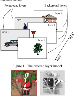
In our proposed approach, a dynamic scene is represented by foreground and background layers. As shown in Figure 1, foreground motion layers are ordered according to their relative depth from front to back. The front-most layer is layer 1. Some background regions, which are defined as the image areas that do not move, may lie in between foreground layers. These background regions are in front of some foreground objects and are called occluding background layers. In our model, as shown in Figure 1, there is one background layer between every two neighboring foreground layers. There is also one background layer that is behind all foreground layers and one layer that is in front all foreground layers (layer 1). If there are L foreground layers, the there are L+1 background layers.

Bac k

Front

Foreground layers Background layers

Layer 1 Layer 2

Layer 3

Layer 1

Layer 2

Figure 1. The ordered layer model.

Figure 2. An example of the background layers. Each foreground layer is described by its motion, shape, and appearance. Each background layer is described by its shape and appearance. If the background also moves, all background layers share a single motion. At any time t,

the set of all layer parameters is called the state of the tracker and is denoted by Λ_t. In later sections, we will describe in detail the models for these state variables. Figure 2 shows a real example of a video frame and the top-most occluding background layer. In this example, only the shape of the front-most background layer is shown. Using the above layer model, from the object point of view, each object belongs to one of the foreground layers. We explicitly model and estimate the layer assignment for the objects in the scene. The depth ordering of L foreground objects at time t is denoted asOt =[i1,i2,...,iL]. The integer variable ij∈[1,L] and

l k i

i ≠ iff k≠l . If we assume that objects do not interleave with each other, there are !L possible layer assignments for L foreground objects. We further assume that the depth ordering is a random variable with a uniform distribution. This means all the permutations have the same probability and thus have the same prior probability

! 1 ) (O, L

P ti = , where Ot,i is an arbitrary layer ordering

configuration.

It should be noticed that the foreground layer ordering, together with the shape, appearance, and motion information of all foreground and background layers, provide the complete information for occlusion reasoning.

2.2 Motion

models

We describe the background motion using a 2D affine model. and estimated this model using the so-called direct method [1]. All background layers share the same motion. Each foreground layer undergoes a 2D rigid motion, which is described using position µ , orientation ω , scaling factor s , and their temporal derivatives. A constant velocity model is used to describe the dynamics of the foreground layers. If we denote the motion parameters of a layer as θ=[µ,ω,s,µ&,ω&,s&], then the motion dynamics is written as ) , : ( ) | ( ₁ N ₁ Q Pθ_t θ_t− = θ_t Φθ_t− (1)

where θt is the motion parameter at time t, Φ is the

standard transition matrix for a constant velocity model, and the notation N(x:µ,R) denotes a multivariate Gaussian distribution with mean µand covariance matrix

R.

2.3 Shape models of the foreground and

background layers

Each foreground or background layer is associated with a shape map. At each pixel location, the value of the shape map is the probability that the object in the layer presenting at that pixel location (it may not be visible though). For the foreground layer j and position x_i at time t, we denote

the value of the shape map as τ_t,j(x_i). For the background layer, we use the notation π_t,j(x_i) to represent its shape map. One difference between the foreground shape map and the background shape map is that for the background, the probabilistic values of all shape maps at each pixel must sum up to 1. This reveals our underlying assumption that there is only one background surface for each pixel. This is a reasonable assumption because even there are more surfaces they will not be observable anyway.

2.3.1 Layer visibility

Once the shape maps are defined for all layers, for each pixel x_i, we can compute the probability that the jth foreground layer is visible. This is the probability of the joint event that background layers 1 to j are absent, foreground layer1 to j−1 are absent, and jth foreground layer presents at x_i. The first probability is −

∑

j₌

l 1 l(xi)

1 π

because there is only one background surface. The second probability is

∏

−₌1 −

1[1 ( )]

j

s τs xi , and the third probability is

) ( _i

j x

τ (for simplicity, we ignore the subscript t). As a result, the probability of the jth foreground layer being visible at xi is

∏

∑

− = = ⋅ − − ⋅ = 1 1 1 )] ( 1 [ ) ) ( 1 ( ) ( ) ( j s s i j l l i i j i j x x x x P τ π τ (2)

Similarly, the probability of observing the j th background layer at xi is

∏

− = − ⋅ = 1 1 , ( ) ( ) (1 ( )) j k k i i j i j B x x x P π τ (3)

and the probability of observing one of the background layers is

∑

+

∏

= − =      − ⋅ = 1 1 1 1 )) ( 1 ( ) ( ) ( L j j k k i i j i B x x x P π τ (4) 2.3.2 Shape dynamics

If we assume the shape of the foreground does not change dramatically, then we can use a constant value Gaussian model to describe the dynamics of the shape changes over time. More specifically,

) ), / ) )( ( ( ); ( ( ) | ) ( ( 2 , , , , 1 , , 1 , τ σ µ ω τ τ γ τ τ j t j t i j t j t i j t j t i j t s x R x N x P & & & − − + = − − ₍₅₎

where γ represents the uncertainty in the shape of the layer. The transformation _{R(−ω&t,j)(xi−µ&t,j)/s&t,j} is used

to align the shape maps.

2.4 Appearance

model

The appearance of foreground layer j is defined in the local coordinate system and is denoted as A_t,j. We assume that the image observation model is a Gaussian distribution with the appearance as the mean, or

) ), ( : ) ( ( )) ( | ) ( (It xi At,j xi N It xi At,j xi 2I P = σ (6)

where σ_I2 is the variance of the image observation. Like the motion and shape models, we also assume that the temporal changes of the layer appearance follow a constant value Gaussian distribution. This is formulated as

) : ) ( : ) ( ( )) ( | ) ( ( 2 , 1 , , 1 ,j i t j i tj i t j i A t x A x N A x A x A P − = − σ (7) where 2 A

σ is the appearance uncertainty that accounts for the appearance variations.

2.5

The MAP estimation

The tracking procedure can be considered as the maximization of the posterior probability

) ,..., , | ( max arg P t t1 It I0 t − Λ Λ Λ (8)

Using Bayes rule and the HMM model,

) | ( ) | ( ) ,..., , | (Λt Λt−1 It I0 =P It Λt ⋅PΛt Λt−1 P (9)

where )P(Λt|Λt₋₁ is the state prior function, and

) | (I_{t t}

P Λ is the likelihood function.

Based on our models in the previous sections, the prior function is computed as appearance motion shape bg shape fg order t t P P P P P P ⋅ ⋅ ⋅ ⋅ = Λ Λ − _ _ 1) | ( (10) where ) | ( ₋₁ = t t order P o o P

∏∏

= = − = L j N i tj i t j i shape fg j x x P P 1 1 , 1, _ (τ ( )|τ ( ))

∏∏

+ = = −

=

1 1 1 , 1 , _

(

(

)

|

(

))

L j N i i j t i j t shape bg j

x

x

P

P

π

π

∏

= −

=

L j j t j t motion

P

P

1 , 1 ,

|

)

(

θ

θ

∏∏

= = − = L j N i tj i t j i appearance j x A x A P P 1 1 , 1, )) ( | ) ( (

Here we assume the image has L foreground layers, L+1 background layers, and N_j pixels on the object in layer j.

To compute the likelihood function, we need to first obtain the probabilistic distribution of the front-most layer at each pixel based on foreground layer ordering, foreground and background shapes, and the appearance models. More specifically, we compute the likelihood function as )) ( ) ( ( ) | ( 1 fgo i N i bgo i t t P x P x I P

∏

= + = Λ (11)

wherePbgo(xi) and Pfgo(xi) represent the likelihood of

one of the background or foreground layers is visible at pixel x_i. They can be computed as

) ( )) ( | ) ( ( ) ( _{i i i B i} bgo x P I x B x P x P = ⋅ (12) and

[

]

∑

= ⋅ = L j j i j i j i i fgo x P I x A x P x P 1 ) ( )) ( | ) ( ( ) ( (13) ) ( i B x

P and P_j(x_i) are defined in Eq(2-4).

3 Estimation of the object state

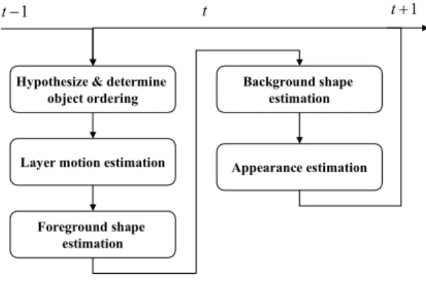
Solving Eq(8) is a difficult optimization problem because the state space is very large. An approximate solution can be found by first decomposing the original problem into several sub-problems (see Figure 3). Then optimization is performed to solve these sub-problems sequentially. We found that in practice this approach yields feasible solutions.

Hypothesize & determine object ordering

Layer motion estimation

Foreground shape estimation Background shape estimation Appearance estimation 1 + t 1 − t t

Figure 3. Estimation of the state parameters.

3.1

Foreground layer ordering hypothesis

Foreground layer ordering Ot is modeled as a uniformly

distributed random variable. Because of this property, the estimation of O_t is rather simple: the algorithm goes through all the possible value of O_t, and finds the one that maximizes the posterior probability. Since all the other parameter estimation steps highly depend on the depth ordering, it is computed at the beginning of each iteration.

3.2 Motion

estimation

Maximizing the posterior probability in Eq(8) w.r.t. foreground layer motion is equivalent to optimizing the function motion i fgo n i bgo i P x P x P + ⋅

∏

= )) ( ) ( ( 1 (14) A search algorithm can be used to find the solution around the predicted position. Rotation, translation, and the scaling factor are discretized with sufficient precision for this purpose. For sequence with moving background, a direct method [1] is used to estimate the motion parameters.

3.3 Foreground

shape

estimation

From Eq(11-13) and Eq(2-4), it can be observed that the likelihood is a linear function of each foreground shape variable τj(xi) and the prior term is a Gaussian function of τj(xi). If we optimize τj(xi) independently for each

layer, the estimation becomes the maximization of a function in the form of

2 2 0) /2σ ( ) (ax+be−x−x (15) where a and b are constants that can be computed using Eq(11-13) and Eq(2-4). The optimal solution is 0, 1, or the root of the quadratic equation

0 ) ( ) ( 0 0 2 2_{+ b−ax x− bx +aσ =} ax (16)

This equation is derived by taking the derivatives of the function in Eq(15) and set it to be 0.

3.4

Background shape estimation

Estimation of the background shape is similar to the estimation of the foreground shape. However, there is one additional constraint needs to be enforced: the values of all shape maps should sum up to 1. With this constraint, the global optimization becomes complicated. However, we can use the results in the previous frame or previous iteration as the starting point to perform a greedy algorithm to find the local optimal solution. We estimate each background level individually with the shape maps of other layers fixed. After all shape values for all layers are estimated, they are normalized so that their sum becomes 1. There is another difference between the background shape estimation and the foreground shape estimation. For foreground, the object shape does not change significantly over time because of the 2D rigid model. Therefore we use the shape in the previous frame as our prior in the estimation. However, in the background shape estimation, the shape of each background layer highly depends on object motion. The occluding background shape in the same area can change quickly from time to time because of object movements. For example, a car may first pass behind a tree, turn around and then pass in front of the tree again; in the first case the tree is part of the occluding

background layer to the foreground layer of car, while in the second case the tree belongs to the background layer that does not occlude the same foreground. So in our algorithm if all the objects leave an area for a certain period of time, we actually lack visual information to infer background layer shapes. As a result, no matter what the previous background shape values are, they becomes obsolete and the shape of all background layers are reset to a default value.

3.5 Appearance

estimation

To estimate the appearance, we need to find A_t,j that maximizes the function

∏

= + ⋅

n

i bgo i fgo i appearance P x P x P 1 )) ( ) ( ( (17)

Since both the appearance observation model Eq(6) and the appearance dynamics Eq(7) are Gaussian functions, the function in Eq(17) becomes a Gaussian mixture. The closed-form solution to this optimization problem is difficult to find. However, appearance is a discrete function and we know the solution should be between the current observation and the previous estimate. For each pixel, we can search for the appearance value in this range to find the solution.

4 Implementation and experimental results

4.1

Initialization and deletion of objects

In addition to the tracking algorithm discussed in the previous sections, there are several other issues regarding the initialization and deletion of the foreground and background layers need to be addressed. In our implementation, change image is computed to determine whether a moving object presents in the scene. A new object is initialized if a change blob is detected far away from any existing objects. In this case, we assume the center of the object is located at the center of the change blob. The value of shape map at each pixel is proportional to the intensity of the change image. The appearance is set to be the original image intensity values. An additional background layer is inserted. The new layer has the same shape map as its neighboring background layer. A normalization step is then applied to make sure these background shape maps sum up to 1 at each pixel.

An object is deleted if it moves out of the image boundaries or it is occluded for a very long period of time. Then the foreground layer of this object is removed from the data structure and two background layers next to it merge into one layer with the shape mask value equal to the sum of the original two shape maps.

4.2 Synthetic

videos

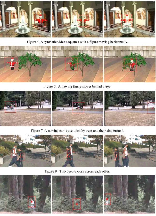
We have tested the proposed algorithm using synthetic and real video clips. (Video clips of the results are

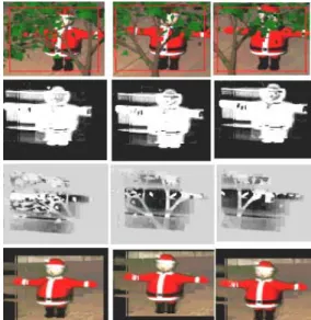
available in the supplementary file). In Figure 4 and Figure 5 show the tracking results of two synthetic videos with moving objects. The videos include difficult conditions including shadows, reflections, and transparent objects (e.g. the waterfall), and out-of-plane object rotation. Our tracking algorithm locked on the moving objects successfully through occlusion in both sequences. The estimated state variables in three key frames of the second video are shown in Figure 6. It can be observed the background shape maps in row 3 accurately describe the shape of the occluding tree.

4.3

Vehicle tracking through occlusion

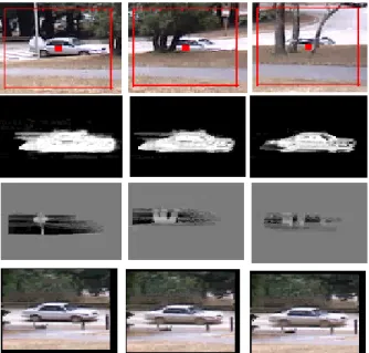
We implemented a tracking system based on the proposed algorithm for handling object occlusions. In Figure 7, the tracking result on a video clip with a car occluded by background is demonstrated. In this example, background objects such as trees, light poles, and the rising ground occlude the car. The proposed tracking algorithm estimates the layer parameters correctly through the sequence. The tracker found one foreground layer and two background layers. The estimated state variables in three key frames are demonstrated in Figure 8. The background shape maps are for the front-most layer.

Figure 6. Layer state variables in three frames of the video in Figure 5 (Row 1 are the original images, Row 2 are the foreground shapes, Row 3 are the background shapes, and Row 4 are the foreground appearances).

4.4 Human

tracking

Although our model of layer shape is 2D rigid, our tracker is able to track moving people by adjusting the system parameters and focusing torso area, which is relatively rigid compared to the other parts of human body. Figure 9 shows the tracking result of two persons passing accross each other. The algorithm tracked both persons successfully through the occlusion.

Figure 10 demonstrates the tracking results on a video clip in which a walking person is occluded by background objects. Because the occluding background area is large, there is a long period of full occlusion. Since the algorithm estimates the background occluding layers, it knows which part of the foreground is occluded. As a result, the tracker is aware of the occlusion and will not update the object appearance. The tracker is able to regain correct values of layer state soon after the object moves out of the occluding background, as observed in the last frame.

Figure 8. Layer state variables in three frames of the video in Figure 7 (Row 1 are the original images, Row 2 are the foreground shapes, Row 3 are the background shapes, Row 4 are the foreground appearances).

5

Conclusions

A novel motion layer based representation and the associated estimation algorithm have been proposed in this paper. This new approach extends the traditional layer model by introducing the background layers and layer ordering. The experimental results demonstrate the power of this representation in handling the difficult occlusion problem in tracking.

One advantage of the proposed representation is that it models all possible interaction between foreground and background objects. Not only the occlusion caused by the foreground layer is modeled, but also modeled is the occlusion caused by the background layers.

Some future research topics for improving the proposed algorithm include the development of more flexible shape

and motion models that can handle articulated and nonrigid motions and the investigation of efficient optimization algorithms for finding the optimal ordering of the foreground layers.

References

[1] J. R. Bergen, P. Anandan, K. J. Hanna, and R. Hingorani,

Hiearchical model-based motion estimation, in Proc. of 2nd

European Conference on Computer Vision, pp. 237-252,

1992.

[2] M.J. Black, D.J. Fleet., and Y. Yacoob A framework for

modeling appearance change in image sequences. IEEE

International Conference on Computer Vision, Mumbai,

India, January 1998, pp. 660-667.

[3] Black, M. J. and Fleet, D. J., Probabilistic detection and

tracking of motion boundaries, Int. J. of Computer Vision,

38(3):231-245, July 2000.

[4] Allan D. Jepson, David J. Fleet, Michael J. Black A Layered Motion representation with occlusion and compact spatial

support. ECCV (1) 2002: 692-706.

[5] Allan D. Jepson, David J. Fleet and Thomas F. El-Maraghi,

Robust online appearance models for visual tracking IEEE

Conference on Computer Vision and and Pattern Recognition,

Kauai, 2001, Vol. I, pp. 415–422.

[6] N. Jojic, N. Petrovic, B. Frey, and T. S. Huang, Transformed hidden Markov models: estimating mixture models of images and inferring spatial transformations in video sequences, in

Proc. of the IEEE Conference on Computer Vision and

Pattern Recognition, pp.(II) 26-33, 2000.

[7] N. Jojic and B.J. Frey Learning flexible sprites in video layers.

In Computer Vision and Pattern Recognition, pp. (I) 199-206,

2001.

[8] L.R. Rabiner. A tutorial on hidden Markov models and

selected applications in speech recognition. Proceedings of

the IEEE, 77(2): 257-285, 1989.

[9] H. Tao, H. Sawhney and R. Kumar, “Object tracking with

Bayesian estimation of dynamic layer representations”, IEEE

Transactions On Pattern Analysis And Machine Intelligence.

Jan. 2002.

[10] N. Vasconcelos and A. Lippman, Emprical Bayesian

EM-based motion segmentation, in Proc. of IEEE Conference on

Computer Vision and Pattern Recognition, pp. 527-532, 1997.

[11] J. Y. A. Wang and Edward H. Adelson, Layered

representation for motion analysis, in Proc. of IEEE

conference on Computer Vision and Pattern Recognition, pp.

361-366, 1993.

[12] Y. Weiss and E. H. Adelson, A unified mixture framework for motion segmentation: incorporating spatial coherence and

estimating the number of models, in Proc. of IEEE conference

on Computer Vision and Pattern Recognition, pp. 321-326,

Figure 4. A synthetic video sequence with a figure moving horizontally.

Figure 5. A moving figure moves behind a tree.

Figure 7. A moving car is occluded by trees and the rising ground.

Figure 9. Two people work across each other.