DISJUNCTIVE NORMAL UNSUPERVISED LDA FOR P300-BASED BRAIN-COMPUTER INTERFACES
by
Majed Elwardy
Submitted to the Graduate School of Engineering and Natural Sciences in partial fulfilment of
the requirements for the degree of Master of Science
Sabanci University August 2016
DISJUNCTIVE NORMAL UNSUPERVISED LDA FOR P300-BASED BRAIN-COMPUTER INTERFACES
APPROVED BY
Assoc. Prof. Dr. M¨ujdat C¸ ET˙IN ... (Thesis Supervisor)
Assoc. Prof. Dr. Tolga TAS¸DiZEN ...
Assoc. Prof. Dr. Kemal KILIC¸ ...
© Majed Elwardy 2016 All Rights Reserved
Acknowledgments
I would like to thank my supervisor M¨ujdat C¸ etin for his guidance, motivation, suggestions and freedom encouragement throughout my graduate studies. It was a great and unforgetable experience to work with him.
I would like to thank Tolga Ta¸sdizen for his guidance, precious suggestions and support on my thesis study and his participation in the Thesis committee.
I would like to thank Kemal Kılı¸c for his support on my graduate courses, mo-tivation and his participation in the Thesis committee.
I am also thankful to T ¨UB˙ITAK for providing the financial support for my grad-uate education and my living support1.
My special thanks to Ozan ¨Ozdenizci, Sezen Ya˘gmur G¨unay, Mastaneh Torka-mani Azar, and Abdullahi Adamu for sharing their BCI experiences with me, for their non-stop help and continuous support during my graduate. I am also thankful to all other members of SPIS group specially O˘guzcan Zengin, Muhammad Usman Ghani, and Muhammed Burak Alver for their unconditional help.
I owe special thanks to my parents (Mahmoud Elwardy & Manal Ali), my wife Zeinab, and my son Omar for their limitless love and support. Without them, I would never have achieved to this point. Although my son is 11 months old during my thesis defence, but he add a lot to me with his laughing, smiling, and crying.
1This work has been supported by a graduate fellowship from the Scientific and Technological
DISJUNCTIVE NORMAL UNSUPERVISED LDA FOR P300-BASED BRAIN-COMPUTER INTERFACES
Majed Elwardy
EE, M.Sc. Thesis, 2016
Thesis Supervisor: M¨ujdat C¸ etin
Keywords: Brain-computer interface, P300 Speller, calibration session, unsupervised classifier, unlabelled data, LDA, BLDA
Abstract
Can people use text-entry based brain-computer interface (BCI) systems and start a free spelling mode without any calibration session? Brain activities differ largely between people and across sessions for the same user. Thus, how can the text-entry system classify the target character among the other characters in the P300-based BCI speller matrix? In this thesis, we introduce a new unsupervised classifier for a P300-based BCI speller, which uses a disjunctive normal form rep-resentation to define an energy function involving a logistic sigmoid function for classification. Our proposed classifier updates the initialized random weights per-forming classification for the P300 signals from the recorded data exploiting the knowledge of the sequence of row/column highlights. To verify the effectiveness of the proposed method, we performed an experimental analysis on data from 7 healthy subjects, collected in our laboratory and used public BCI competition datasets. We compare the proposed unsupervised method to a baseline supervised linear discrim-inant analysis (LDA) classifier and Bayesian linear discrimdiscrim-inant analysis (BLDA) and demonstrate its performance. Our analysis shows that the proposed approach facilitates unsupervised learning from unlabelled test data.
P300 TABANLI BEY˙IN-B˙ILG˙ISAYAR ARAY ¨UZLER˙I ˙IC¸ ˙IN AYIRICI NORMAL G ¨OZET˙IMS˙IZ DAA
Majed Elwardy
EE, Y¨uksek Lisans Tezi, 2016
Tez Danı¸smanı: M¨ujdat C¸ etin
Anahtar Kelimeler: Beyin-bilgisayar aray¨uz¨u, P300 heceleyicisi, ayarlama oturumu, g¨ozetimsiz sınıflandırıcı, etiketsiz veri, DAA, BDAA
¨
Ozet
˙Insanlar metin yazma ama¸clı beyin-bilgisayar aray¨uz¨u (BBA) sistemleri i¸cin ayarlama oturumuna ihtiya¸c duymadan do˘grudan heceleme moduna ge¸cebilirler mi? Beyin aktiviteleri insanlar arasında ve aynı kullanıcının farklı oturumları arasında b¨uy¨uk degi¸skenlik g¨ostermektedir. Bu durumda metin yazma sistemleri P300 tabanlı BBA heceleme matrisindeki hedef harfi di˘gerlerinden ayırt ederek nasıl sınıflandırabilir? Biz bu tezde P300 tabanlı BBA heceleyicileri i¸cin yeni bir g¨ozetimsiz sınıflandırıcı ¨
oneriyoruz. Bu sınıflandırıcı lojistik sigmoid fonksiyonuna dayalı bir enerji fonksiy-onu tanımlamak i¸cin ayırıcı normal form temsili kullanıyor. ¨Onerdi˘gimiz sınıflandırıcı satır/s¨utunların parlakla¸stırılarak vurgulanma dizisine dair bilgileri kullanarak, kaydedilen verilerden P300 sinyallerini sınıflandırmak i¸cin rastgele olarak ba¸slatılan a˘gırlıkları g¨unceller. ¨Onerilen y¨ontemin ge¸cerlili˘gini do˘grulamak i¸cin kendi laboratuvarımızda toplanan ve kamuya a¸cık BBA yarı¸sması veri k¨umelerinde bulunan 7 sa˘glıklı kul-lanıcıya ait veriler ¨uzerinde bir deneysel analiz ger¸cekle¸stirdik. ¨Onerdi˘gimiz g¨ozetimsiz y¨ontemi temel d¨uzeyde birer g¨ozetimli sınıflandırıcı olan do˘grusal ayırta¸c anal-izi (DAA) ve Bayes¸ci do˘grusal ayırta¸c analizi (BDAA) ile kar¸sıla¸stırıp ba¸sarımını g¨osterdik. Analizimiz ¨onerilen yakla¸sımın etiketsiz test verilerinden g¨ozetimsiz ¨o˘grenmeyi kolayla¸stırdı˘gını g¨osterdi.
Table of Contents
Acknowledgments v Abstract vi ¨ Ozet vii 1Introduction
1
1.1 Scope . . . 1 1.2 Motivation . . . 3 1.3 Contributions . . . 4 1.4 Outline . . . 52
Background on BCI and P300 Spellers
6
2.1 Introduction . . . 62.2 Electroencephalography (EEG) Signals . . . 7
2.2.1 Electrodes . . . 7
2.3 A Journey to General BCI Systems . . . 10
2.3.1 Motor Imagery . . . 10
2.3.2 Event Related Potentials . . . 11
2.4 P300-based BCI Systems . . . 14
2.4.1 Decoding the Brain Signals for A P300-based BCI System . . 18
2.5 Machine Learning for P300 Speller . . . 19
2.5.1 Supervised Learning . . . 19
2.5.2 Unsupervised Learning . . . 21
2.6 Summary . . . 24
3
Disjunctive Normal Unsupervised Classifier
25
3.1 Linear Discriminant Analysis (LDA) . . . 253.2 Bayesian Linear Discriminant Analysis (BLDA) . . . 26
3.3 Disjunctive Normal Unsupervised LDA classifier (DNUL) . . . 29
3.3.1 Model Architecture . . . 29
3.3.2 Model Initialization . . . 30
3.3.3 Model Optimization . . . 31
3.4 Regularized Disjunctive Normal Unsupervised LDA Classifier (RD-NUL) . . . 31
4
Offline and Simulated Online Analysis Experiments
38
4.1 Background . . . 38 4.2 Terminology . . . 39 4.3 P300 Classification Problem . . . 40 4.4 Methods . . . 41 4.4.1 Data pre-processing . . . 41 4.4.2 Classification . . . 43 4.5 Dataset . . . 43 4.6 Experimental Setup . . . 44 4.7 Experimental Results . . . 45 4.7.1 Offline Analysis . . . 464.7.2 Simulated Online Analysis . . . 72
4.8 Comparison with the State-of-the-art in Unsupervised Classification in BCIs . . . 78
5
Conclusion and Future Work
86
A Datasets 89
B Sensitivity Parameter (β) 92
List of Figures
1.1 (a) A BCI-based motor imagery system. (b) A BCI-based P300 speller. 2
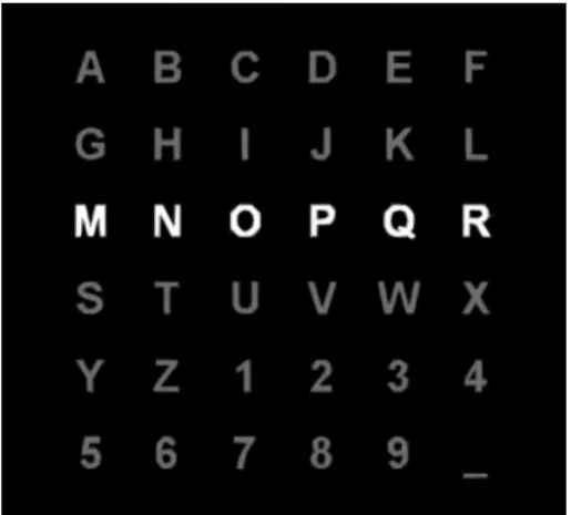
1.2 Interface of P300-based speller matrix used in this study. . . 3
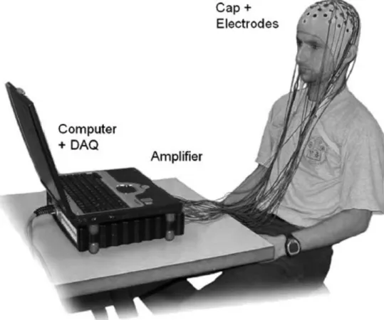
2.1 A typical EEG based BCI system consists of electrodes, cables, am-plifier, and a computer that processes the data. Taken from [1]. . . . 8
2.2 64-channel electrode cap using international 10-20 electrode distribu-tion. Taken from [2] . . . 9
2.3 Active electrodes and gel used in this study. Taken from [3] . . . 9
2.4 The international 10-20 system. Taken from [1]. . . 9
2.5 A typical BCI system model. Taken from [4]. . . 11
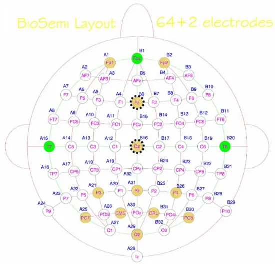
2.6 Electrode placement layout according to the 10-20 electrode system. The dashed black circles show the location of highest amplitude of the P300 component. The golden electrodes are used in this work. CMS and DRL electrodes form a feedback loop, which drive the av-erage potential of the subject (the Common Mode voltage) as close as possible to the ADC reference voltage. Taken from [5] . . . 13
2.7 Average of (Subject 5) brain signals over trials following a visual stimulus obtained from different electrode sites. The solid red line is the average response of trials where a P300 wave is visible, the blue dashed line shows the average response of trials where no P300 wave is elicited. . . 14
2.8 First P300 speller paradigm used by Farwell and Donchin. . . 15
2.9 Two different paradigms (a) Hex-o-Spell interface. (b) RSVP key-board interface. . . 16
2.10 The user interface of the AMUSE paradigm. Each circle encodes one out of six tones/tone directions relative to the user, who is positioned in the middle of the ring of speakers [6] . . . 17 2.11 Elements of the user’s screen. Text To Spell indicates the pre-defined
text. The speller will analyze evoked responses, and will append the selected text to Text Result. [7] . . . 17 2.12 SU-BCI P300 Stimulus Software used in this study. . . 18 2.13 A hyperplane which separates two classes. Taken from [8] . . . 20 2.14 Three examples of data generated by the LDA model. Note that in
LDA both classes share the same covariance structure. To show the influence of the covariance structure on the direction of the decision boundary, we have used the same means per class in all three exam-ples. By changing the covariance structure over the three examples, we rotate the decision boundary. An example can be seen in [9]. . . . 20 2.15 Example of data generated from a three component Gaussian Mixture
Model. Note that unlike data generated by an LDA model, each cluster has its own covariance structure. Example in [9]. . . 23
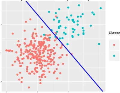
3.1 A toy example on a synthetic dataset with a standard deviation = 0.2. The DNUL classifier classified the data successfully with 100% classification accuracy. The second figure shows the energy function for the initialized 2 random-weight vectors for one of the classifiers among 10 classifiers (which is the highest). . . 34 3.2 A toy example on a synthetic dataset with a standard deviation =
0.4. The classifier achieved 97.76% classification accuracy with true positive rate = 94.23% and true negative rate = 97.69%. . . 35 3.3 A toy example on a synthetic dataset with a standard deviation =
0.5. The classifier achieved 95.19% classification accuracy with true positive rate = 82.69% and true negative rate = 98.46%. . . 35 3.4 A toy example on a synthetic dataset with a standard deviation =
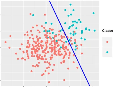
0.6. The classifier achieved 91.67% classification accuracy with true positive rate = 71.15% and true negative rate = 95.76%. . . 36
3.5 A toy example on a synthetic dataset with a standard deviation = 0.7. The classifier achieved 90.71% classification accuracy with true positive rate = 69.23% and true negative rate = 95%. . . 36 3.6 A toy example on a synthetic dataset with a standard deviation =
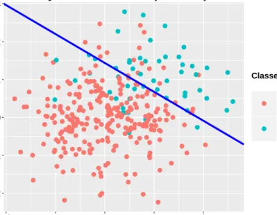
0.8. The classifier achieved 87.18% classification accuracy with true positive rate = 63.46% and true negative rate = 91.92%. . . 37 3.7 A toy example on a synthetic dataset with a standard deviation =
0.9. The classifier achieved 86.56% classification accuracy with true positive rate = 61.53% and true negative rate = 91.53%. . . 37
4.1 Offline analysis results for subject 1 with (Batch-26) configuration. . . 47 4.2 Offline analysis results for subject 2 with (Batch-26) configuration. . . 48 4.3 Offline analysis results for subject 3 with (Batch-26) configuration. . . 48 4.4 Offline analysis results for subject 4 with (Batch-26) configuration. . . 48 4.5 Offline analysis results for subject 5 with (Batch-26) configuration. . . 49 4.6 Offline analysis results for subject 6 with (Batch-26) configuration. . . 49 4.7 Offline analysis results for subject 7 with (Batch-26) configuration. . . 49 4.8 Average classification performance over 7 subjects with (Batch-26).
Error shadows show 95% confidence intervals from the mean with sample size = 7. . . 50 4.9 Offline analysis results for subject 1 with (Batch-14) configuration. . . 51 4.10 Offline analysis results for subject 2 with (Batch-14) configuration. . . 51 4.11 Offline analysis results for subject 3 with (Batch-14) configuration. . . 52 4.12 Offline analysis results for subject 4 with (Batch-14) configuration. . . 52 4.13 Offline analysis results for subject 5 with (Batch-14) configuration. . . 52 4.14 Offline analysis results for subject 6 with (Batch-14) configuration. . . 53 4.15 Offline analysis results for subject 7 with (Batch-14) configuration. . . 53 4.16 Average classification performance over 7 subjects with (Batch-14).
Error shadows show 95% confidence intervals from the mean with sample size = 7. . . 53 4.17 Offline analysis results for subject 1 with (N-Batch-26) configuration. 55 4.18 Offline analysis results for subject 2 with (N-Batch-26) configuration. 55 4.19 Offline analysis results for subject 3 with (N-Batch-26) configuration. 55
4.20 Offline analysis results for subject 4 with (N-Batch-26) configuration. 56 4.21 Offline analysis results for subject 5 with (N-Batch-26) configuration. 56 4.22 Offline analysis results for subject 6 with (N-Batch-26) configuration. 56 4.23 Offline analysis results for subject 7 with (N-Batch-26) configuration. 57 4.24 Average classification performance over 7 subjects with
(N-Batch-26). Error shadows show 95% confidence intervals from the mean with sample size = 7. . . 57 4.25 Offline analysis results for subject 1 with (N-Batch-14) configuration. 58 4.26 Offline analysis results for subject 2 with (N-Batch-14) configuration. 59 4.27 Offline analysis results for subject 3 with (N-Batch-14) configuration. 59 4.28 Offline analysis results for subject 4 with (N-Batch-14) configuration. 59 4.29 Offline analysis results for subject 5 with (N-Batch-14) configuration. 60 4.30 Offline analysis results for subject 6 with (N-Batch-14) configuration. 60 4.31 Offline analysis results for subject 7 with (N-Batch-14) configuration. 60 4.32 Average classification performance over 7 subjects with
(N-Batch-14). Error shadows show 95% confidence intervals from the mean with sample size = 7. . . 61 4.33 Average classification performance comparing the regularized DNUL
classifier with DNUL. Error shadows corresponding to the point show 95% confidence intervals from the mean with sample size = 7. . . 62 4.34 Bit rate performance comparing the regularized DNUL classifier with
DNUL. Error shadows corresponding to the point show 95% confi-dence intervals from the mean with sample size = 7. . . 63 4.35 Average classification performance for subject A over 5 classifier groups
using 12 electrodes with a batch mode configuration. . . 65 4.36 Average classification performance for subject A over 5 classifier groups
using 64 electrodes with a batch mode configuration. . . 65 4.37 Classification performance for subject A using 12 electrodes with a
N-batch mode configuration. . . 66 4.38 Classification performance for subject A using 64 electrodes with a
4.39 Average classification performance for subject B over 5 classifier groups using 12 electrodes with a batch mode configuration. . . 67 4.40 Average classification performance for subject B over 5 classifier groups
using 64 electrodes with a batch mode configuration. . . 67 4.41 Classification performance for subject B using 12 electrodes with a
N-batch mode configuration. . . 68 4.42 Classification performance for subject B using 64 electrodes with a
N-batch mode configuration. . . 68 4.43 Average classification performance for subject C over 5 classifier groups
using 12 electrodes with a batch mode configuration. . . 69 4.44 Average classification performance for subject C over 5 classifier groups
using 64 electrodes with a batch mode configuration. . . 69 4.45 Classification performance for subject C using 12 electrodes with a
N-batch mode configuration. . . 70 4.46 Classification performance for subject C using 64 electrodes with a
N-batch mode configuration. . . 70 4.47 An arbitrary example shows a sequence of letters for simulated online
spelling. . . 72 4.48 Simulated online spelling (sequential mode) showing the performance
averaged over the 7 subjects. . . 74 4.49 Simulated online spelling using 12 electrodes and 64 electrodes for
subject A. . . 75 4.50 Simulated online spelling using 12 electrodes and 64 electrodes for
subject B. . . 76 4.51 Simulated online spelling using 12 electrodes and 64 electrodes for
subject C. . . 77
B.1 A sensitivity parameter analysis showing the classifier performance averaged over the 7 subjects. The x-axis represents the beta value (β). The y-axis represents the classifier accuracy. The shaded band shows the standard error from the mean. The vertical green dashed line intercepts the beta value at 0.1 which gives the maximum classifier accuracy among all values. . . 92
List of Tables
2.1 Methods used for brain-computer interfaces. Taken from [10]. . . 7
3.1 Influence of the tuning parameter. . . 32
4.1 Percentage of correctly classified characters for each subject obtained with different values of trial groups for (Batch-26). . . 47 4.2 Percentage of correctly classified characters for each subject obtained
with different values of trial groups for (Batch-14). . . 50 4.3 Percentage of correctly classified characters for each subject obtained
with different values of trial groups for (N-Batch-26). . . 54 4.4 Percentage of correctly classified characters for each subject obtained
with different values of trial groups for (N-Batch-14). . . 58 4.5 Batch mode: percentage of correctly classified characters for
sub-jects A, B, and C for 12 electrodes. The values in braces are the standard deviation. . . 71 4.6 Batch mode: percentage of correctly classified characters for
sub-jects A, B, and C for 64 electrodes. The values in braces are the standard deviation. . . 71 4.7 N-Batch mode: percentage of correctly classified characters for
sub-jects A, B, and C for 12 and 64 electrodes configuration. . . 72 4.8 Averaged accuracies of our proposed unsupervised classifier (DNUL).
The numbers show the percentage of correctly classified characters. The values in braces are the standard deviation. . . 80 4.9 Averaged accuracies of the competing unsupervised classifier. The
numbers show the percentage of correctly classified characters. The values in braces are the standard deviation. Taken from Kindermans et al. [11] . . . 81
4.10 Accuracies of different supervised classifiers. The numbers show the percentage of correctly classified characters. eSVM, SUP, and
OA-SUP are taken from Kindermans et al. [11]. . . 81
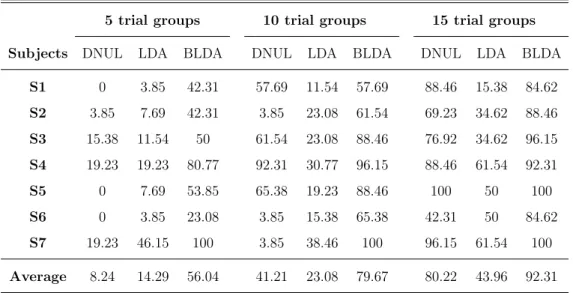
4.11 OFF-US: percentage of correctly classified characters through 10 classifier groups. . . 83
4.12 OFF-US-T: percentage of correctly classified characters through 10 classifier groups. . . 83
4.13 ON-US-T: percentage of correctly classified characters through 10 classifier groups. . . 84
4.14 OA-US-T: percentage of correctly classified characters through 10 classifier groups. . . 84
4.15 RE-OA-US-T:percentage of correctly Percentage of correctly clas-sifiedlassified characters through 10 classifier groups. . . 85
4.16 OA-US:percentage of correctly classified characters through 10 clas-sifier groups. . . 85
A.1 Target words in training and test datasets for SU datasets . . . 90
A.2 Target words in training and test datasets for BCI Competition II . . 90
B.1 Sensitivity parameter (β): SU Dataset (S1) . . . 93
B.2 Sensitivity parameter (β): SU Dataset (S2) . . . 94
B.3 Sensitivity parameter (β): SU Dataset (S3) . . . 95
B.4 Sensitivity parameter (β): SU Dataset (S4) . . . 96
B.5 Sensitivity parameter (β): SU Dataset (S5) . . . 97
B.6 Sensitivity parameter (β): SU Dataset (S6) . . . 98
Chapter 1
Introduction
Across all ages and cultures, people are doing their best to use multiple means to communicate and control, from the beginning of creation to the current era. Talking, writing, and gesture have been the most common ways to interact with each other throughout time. Interestingly, in each era, intellectuals thought about potential barriers and how to overcome them, at least theoretically. For example, a short time ago, back in the 60s, communicating and controlling devices with brain waves was listed as science fiction. In today’s world, it became true and people can communicate with the computer through brain waves. A brain-computer interface (BCI) aims to establish a direct communication channel between the brain and a computer or machine so disabled individuals can interact with the real-world [12].
In this thesis, we introduced a new unsupervised classifier for a P300-based BCI, which tackle some main problems for the text entry systems. These problems can be briefly addressed under the calibration sessions where they are tedious, time-consuming, and annoying sessions for the subjects especially the disabled individu-als. Furthermore, we demonstrate the use of our proposed approach on offline and simulated online analysis in order to verify the effectiveness of the proposed method.
1.1
ScopeTechnology should always improve life quality. A significant number of indi-viduals suffer from losing all voluntary muscle control due to amyotrophic lateral sclerosis (ALS), traumatic brain injuries, or spinal cord injuries [13]. Although the motor pathway is lost, neuronal activity of the brain still works in many of these cases. Therefore, one direction for raising the life quality of the disabled individuals
is to create a channel between a brain and a computer which it can be used for various applications. Thus, BCI returns hope to many people.
Over the last two decades, a large body of work has been performed for recording activity from the brain either invasively or non-invasively for the purpose of brain-computer interfacing. The electroencephalogram (EEG) is a non-invasive technique involving electrical signals measured through the scalp and can be used as the cor-nerstone for BCI [14]. Along with EEG [15], magnetoencephalography (MEG) [16], positron emission topography (PET) [17], functional magnetic resonance imaging (fMRI) [18], and optical imaging, functional near infrared spectroscopy (fNIRS) [19] provide other ways to monitor brain activity non-invasively. In an EEG-based BCI system, incoming signals from an EEG amplifier are processed and classified to de-code the user’s intent [20]. Furthermore, it can be used to provide input signals in many applications including text entry systems [21], robotic arm control [22], and cursor control [23]. Figure 1.1 shows how data are collected from subjects.
One of the most common application related to BCI is the text-entry systems. They allow subjects to select characters from a symbolic grid matrix containing characters and symbols on a computer screen while recording the brain waves. The P300 speller is one of the most common BCI-based text-entry systems, which allows subjects to write text on the computer screen. Farwell and Donchin [21] demon-strated the first P300 speller paradigm which is also called the oddball paradigm. P300 is an event-related potential (ERP) elicited in the brain as a response to a visual or auditory stimulus. It is a positive deflection measured around the parietal
(a) (b)
Figure 1.2: Interface of P300-based speller matrix used in this study.
lobe, nearly 300 ms to 600 ms after the occurrence of the attended stimulus [24]. The system allows people to spell words and numbers by focusing on the desired character or number in a matrix shown on the screen (see Figure 1.2). When the desired character is highlighted, the subject attends to the unexpected stimulus and a P300 wave is generated. The character which the user intends to type can be inferred from the intersection of the detected P300 responses in the sequence of row/column highlights. Machine learning algorithms can be used to classify and learn the attended and non-attended highlights for rows and columns. Thus, the character can be estimated from the intersection of attended highlights.
EEG signals suffer from low signal to noise ratio (SNR) due to several factors including the variability in brain activities, changes in electrode positions in long ses-sions, meta-activities in the brain, and artifacts due to eye movements and muscular activities. Therefore, P300 spellers need several stimulus repetitions to increase the classification accuracy [25] [26].
1.2
MotivationOne of the most common problems in BCIs is the calibration process. Subjects have to go through tedious, time-consuming and annoying calibration sessions before they can start using a BCI system for communication purposes. The brain signals vary across people and across sessions for the same user [27]. For this reason, supervised training methods based on calibration sessions involving labelled training data are usually used. Furthermore, the BCI system should be trained for a specific
person. The downsides of having to use such sessions include the consumption of additional time and increased fatigue for the users. Even for healthy people the calibration is still an annoying process. Furthermore, such sessions might have to be repeated to account for any non-stationary behaviour of the brain signals over the course of system use. The aforementioned problems imply another inherent problem, namely the collected training data may sometimes be unreliable. For example, during the data collection for this thesis, many users reported that they felt sleepy, lost concentration, and probably could not focus on the target letters. Mainly the labelled data is what we expect the user to write, not the user actual writes. Healthy subjects can report mistakes and express feelings during the experiment, then we can decide how reliable the data are. On the other hand, paralyzed people can not express when they made mistakes and it is hard to measure the reliability of the data.
There have been few pieces of work on unsupervised methods for P300-based BCI spellers to tackle the problems raised above. An unsupervised method was proposed by Lu et al. [28]. Although that unsupervised classifier has also been applied to P300 data, it still needs some labelled data from many previous subjects to train a subject independent classification model (SICM), which allows EEG from a new subject to be classified first by the SICM then goes through adaptation process. Another recent unsupervised classification method, based on a Bayesian model, has been proposed by Kindermans et al. [11]. The classifier can be trained unsupervisedly using an Expectation Maximization (EM) approach, eliminating the use of calibration sessions. Up to my knowledge, it was the only paper which is able to train a P300 classifier without any labelled data. There also exist semi-supervised adaptation methods which involve supervised training followed by adaptation of the classifier with the incoming EEG data [29].
1.3
ContributionsThe work done in this thesis provides a contribution towards addressing the men-tioned problems by proposing a new unsupervised classifier for P300-based spellers. In this approach, the disjunctive normal form plays a role in forming an energy function, which allows to update the randomly initialized classifier weights by using
the logistic sigmoid function for classification and by exploiting the knowledge of the sequence of row/column highlights [30]. The idea is that one round of row/column highlights in the speller matrix should evoke a P300 response only after two (one row and one column) of the highlights. Note that exploiting this fact does not require knowledge of the labels of the data, hence this idea can be a basis for unsupervised learning.
To achieve this goal, we propose a disjunctive normal unsupervised LDA for P300-based brain-computer interfaces 1. The thesis makes several contributions,
which can be summarized as follows. We developed a novel unsupervised method based on the disjunctive normal form for P300-based BCI speller systems, which allows us to run the classifier without using any calibration process and without any labelled data. Moreover, we demonstrated the use of our proposed approach on both offline and simulated online analysis experiments. Besides, we compared our classifier with BCI competition datasets (BCI Competition II [32] and BCI competition III [33]).
1.4
OutlineChapter 2 presents introductory background information about BCI, P300 speller paradigm, stimulus software used in this work, and a survey of machine learning techniques used for P300.
Chapter 3 presents the proposed unsupervised classifier and all the supervised classification technical pieces involved in this work together with their mathematical preliminaries.
Chapter 4 presents the offline and simulated online experiments for P300 speller, in order to demonstrate the proposed classifier effectiveness. The perfor-mance and detailed report results can be found in this chapter.
Chapter 5 provides a summary of the contributions made and indicates possi-ble directions for future work, motivated by the limitations and advantages of the proposed methods.
1A preliminary portion of this work was published at the IEEE 24th Signal Processing and
Chapter 2
Background on BCI and P300 Spellers
This chapter aims to provide the basic concepts of EEG signals processing, brain-computer interfaces (BCIs), P300 signals of event-related potentials (ERP) and P300-based spellers, motor imagery systems, and classification methods in both supervised and unsupervised domains. It also includes a survey of published works, methods, and results.
2.1
IntroductionBCI might use brain signals recorded by a variety of methodologies. These include invasive and non-invasive methods. Scalp-recorded EEG provides the most practical and widely used non-invasive access to the brain activity. However, its signal resolution is low. On the other hand, using invasive techniques such as electro-corticography (ECoG), require access to the cortical surface of the brain. Although this technique provides high resolution signals, it is prohibitively expensive and might involve risks for the patient [20].
Most BCIs rely on sensors outside the head to measure the electrical activity of the brain. Magnetoencephalography (MEG), functional magnetic resonance imag-ing (fMRI), and positron emission tomography (PET) are non-invasive rather than (ECoG) which is an invasive. However, they are expensive, hard to utilise outside the laboratory, and not applicable in daily life [20]. In contrast, EEG is relatively cheap, applicable with many different paradigms and offers non-muscular communication and control mechanisms. Table 2.1 shows the methods used for brain-computer Interfaces.
EEG MEG fMRI ECoG
Deployment Noninvasive Noninvasive Noninvasive Invasive Measured activity Electrical Magnetic Hemodynamic Electrical
Temporal resolution Medium Medium Low High
Spatial resolution Low Low Medium Medium
Portability High Low Low High
Cost Low High High High
Table 2.1: Methods used for brain-computer interfaces. Taken from [10].
2.2
Electroencephalography (EEG) SignalsEEG is one of the well-known technique due to its advantages of low cost, non-invasiveness, portability, and ease of use. Because of that, it has become the most commonly used BCI signal acquisition tool. EEG has been mainly used for clinical diagnosis of neurological disorders. EEG signals provide a good temporal resolution (in milliseconds). It measures the electrical activity as voltage changes on the scalp via the electrodes attached to it. Hans Berger introduced human EEG in 1929 [34]. However, EEG is not without disadvantages: EEG signals suffer from poor spatial resolution because of measuring the electrical activities from the scalp as it is an invasive method.
To establish a BCI channel, the electrodes must be placed on the scalp by the cap to detect the EEG signals (5-20 microvolt range). Then, it can be connected to the amplifiers to magnify the EEG signals. Finally, actual brain signals are recorded by a device and converted to a digital format. A typical EEG based BCI system is illustrated in Figure 2.1.
2.2.1
ElectrodesOne of the most important components of BCI systems are electrodes. Electrodes are little pin-pads of Ag/AgCl attached to the scalp with the aid of a headcap consisting of an elastic cap with plastic, electrode holders. An example of the headcap used in our laboratory can be seen in Figure 2.2. In order to decrease
Figure 2.1: A typical EEG based BCI system consists of electrodes, cables, amplifier, and a computer that processes the data. Taken from [1].
the skin resistance or voltage offset and to have a stable, stationary conductive medium for proper measurements, usually a conductive gel is applied to fill the plastic holes before clicking the active electrodes as shown in Figure 2.3. However, electromagnetic interference, power cable noise, and signal degradation, need for skin preparation, etc., are problems for practical usage of these electrodes outside the laboratory [35]. To reduce some of these effects, high active electrode impedance and cable shielding is used as shown in Figure 2.3.
The electrodes are placed on the head of the subject according to an international system called 10-20 system, proposed by the American EEG society [36]. It is widely used in clinical EEG recording and EEG research as well as BCI research. This system proposes that the electrodes are placed in a 10% - 20% distance from each other with respect to the total distance between the nasion and inion of the subject. The labels of the electrode sites are usually also the labels of the recorded channels. Figure 2.4 depicts the electrode placement according to the 10 - 20 system.
Figure 2.2: 64-channel electrode cap using international 10-20 electrode distribution. Taken from [2]
Figure 2.3: Active electrodes and gel used in this study. Taken from [3]
2.3
A Journey to General BCI SystemsIn order to activate the neurons in the brain to elicit electrical signals, it does not require an interference or an effort from the user. Daily life activities such as thinking, moving, feeling something, etc., unconsciously do that itself. Further-more, the neurons will translate the activities of the physiological and pathological information in terms of electrical signals [37]. Those electrical signals recorded by electrodes can be measured and acquired by a bio-signal acquisition system. Then the signals are analyzed to translate the brain activities into command signals using a computer algorithm. These commands can be used to provide input signals in many applications including text entry [21], robotic arm control [22], cursor control [23]. As shown in Figure 2.5, the BCI system usually consists of three main parts: Signal Acquisition, Signal Processing, and Application Interface.
Signal Acquisition involves collecting temporal EEG data and amplifying brain signals. It uses active or passive electrodes to transmit the electrical activity of the subject to a high sensitivity, low-noise amplifier, namely the EEG amplifier. The Signal Processing part then processes the acquired brain signals in three steps sequentially: data pre-processing, feature extraction, and classification or detection. The processed data is transmitted into the Application Interface part for further control of external devices or any other useful clinical applications like treating stroke, autism, and other disorders.
2.3.1
Motor ImageryMany BCI systems rely on imagined movement. The brain activity changes in the EEG recording either with real or imagined movement. That advance the ability of people to record and use BCIs with their mental state tasks. The EEG signals are recorded multiple times from the brain processes. The information is averaged over the different recordings to filter out redundant brain activity and to keep the relevant information [38]. Most of the motor imagery data belong to two classes such as mentally thinking about moving left and right hand[39]. Besides, it allows subjects to have binary communication to choose between two categories by just thinking of right and left hand movements.
Figure 2.5: A typical BCI system model. Taken from [4].
alpha rhythm and the central mu and beta rhythms. In motor imagery studies, spectral power densities around 16-24 Hz for beta, 12-16 Hz for sigma, 8-12 Hz for alpha bands are used. A calibration session or adaptivity method is needed to train or adapt the computer to differentiate between the different classes.
2.3.2
Event Related PotentialsAn event-related potential (ERP) is a specific brain response to an event such as the presentation of a visual or auditory stimulus (e.g., a specific flash or sound), a mistake, a motor event [40]. It is an unconsciously stereotyped brain wave recorded on the scalp. ERPs can be measured before, during or after sensory, motor or psychological events and usually have a fixed time delay after (or before) these events, named stimuli. In 1964, Walter et al. discovered that when a subject was required to press a button after detecting a target in a visual stimulus, they elicited a large negative voltage at frontal electrodes that happen just before the subject presses the button [41]. This voltage, ERP component called Contingent Negative
Variation (CNV) indicated the subject’s mental preparation to press the button. One of the most extensively used ERP component in BCI research is P300, usually named P300 component discovered by Sutton et al. in 1965 [42]. This thesis is focused and completely related to the P300 component. This component will be discussed in the next section.
P300 component
P300 is an event-related potential (ERP) elicited in the brain as a response to a visual or auditory stimulus. It is a large positive deflection measured around the parietal lobe, nearly 300 ms to 600 ms after the occurrence of the attended stimulus [24]. This idea generated another paradigm known as the ‘oddball paradigm’, where the subject is stimulated with two categories of events: relevant and irrelevant [43]. The relevant events occur rarely with respect to irrelevant events, and due to the complete random order of events, elicit a large P300 response in ERPs. For the first time in 1988, Farwell and Donchin used the oddball paradigm to devise a communication system which allows users to type letters on a screen by thoughts with P300 signals rather than using muscular output [21].
Donchin and his colleagues developed a 6×6 matrix of letters, numbers, and/or other symbols. The individual rows and columns flash in a block-randomized fashion and the user attends to the desired item and counts how many items it flashes. Here the row and column which contain the target letter are the relevant events or target stimuli, while other are irrelevant events or non-target stimuli.
The P300 component is located along the mid-line scalp sites. The highest amplitudes of the P300 component can be recorded from central-parietal (Cz) and mid-frontal (Fz) electrode locations [44]. Figure 2.6 shows the electrode placement layout used in this work according to the 10-20 electrode placement system. Figure 2.7 shows a typical P300 response of a single trial and averaged over trials recorded at several electrode sites used in this work.
As can be seen from that section, recording the P300 component looks easy. Nevertheless, the quality of P300 signals is affected by various factors as following:
• Positioning a cap toward the correct location plays a role with signals quality including P300 components.
Figure 2.6: Electrode placement layout according to the 10-20 electrode system. The dashed black circles show the location of highest amplitude of the P300 component. The golden electrodes are used in this work. CMS and DRL electrodes form a feedback loop, which drive the average potential of the subject (the Common Mode voltage) as close as possible to the ADC reference voltage. Taken from [5]
• A subject’s mental state, emotion, psychological activities, degree of fatigue, and concentration will all affect the result of P300 recordings.
• The recording environment of the temporal EEG data will also influence the final acquisition of a P300 signal. The surrounding noise should be reduced in order to achieve a high quality P300 signal. A P300 signal is always averaged by several measurements due to its small amplitude (in µv).
Figure 2.7: Average of (Subject 5) brain signals over trials following a visual stimulus obtained from different electrode sites. The solid red line is the average response of trials where a P300 wave is visible, the blue dashed line shows the average response of trials where no P300 wave is elicited.
2.4
P300-based BCI SystemsThe first ERP-based BCI system that was produced is the P300-based BCI by Farwell and Donchin (1988), also known as the matrix speller. The matrix speller consists of a 6×6 grid of symbols which are shown on the computer screen. Figure 2.8 shows the first prototype of the P300 speller paradigm. Donchin’s first P300 speller has become the most widely studied P300 based BCI system [21]. It can be seen from the Figure 2.8 that it has 36 cells, involves 26 letters, 6 commands, and 4 symbols. The task here is to spell the word “B-R-A-I-N” letter by letter using the matrix speller paradigm shown at the top of Figure 2.8. By focussing attention on a specific symbol, the subject is able to select that symbol. The speller matrix is covered by a random flash sequence. If the the row or column with the target character is flashed, then a P300 signal will occur. The other flashes with the non-target characters are then considered as irrelevant targets and no P300
Figure 2.8: First P300 speller paradigm used by Farwell and Donchin.
signals will appear. Besides, using feature selection and classification techniques for P300 signals aid the system to predict the character and display it on the computer screen. In a few cases the computer displayed a letter other than the one in which a subject was focusing, then the subject focused on the BKSP (backspace) command to delete the character in order to correct the error. At the end, the subject selected the TALK command and a computer read the spelled word [21].
P300-based BCI systems and related technologies have been highly developed and improved recently. Many paradigms including flashing, stimulus techniques, and interfaces have been introduced. One example of this is the hexagonal two-level hierarchy of the Berlin BCI known as “Hex-o-Spell” [45], where characters are clustered based on hexagons appealing visualization as shown in Figure 2.9 (a). Another introduced paradigm is the rapid serial visual presentation (RSVP) keyboard. It allows visual stimulus sequences to be displayed on a screen over time on a fixed focal area and in rapid succession [46]. RSVP keyboard paradigm can be seen in Figure 2.9 (b).
An auditory ERP-based paradigm, called AMUSE, is introduced in [47]. In AMUSE, each stimulus is a specific tone that originates from a specific direction. Kindermans et al., used 6 unique tones forming auditory stimuli, each produced by one of six speakers that are positioned on a ring of 130 cm diameter around the user. Figure 2.10 shows the user interface used in this study [6].
(a) (b)
Figure 2.9: Two different paradigms (a) Hex-o-Spell interface. (b) RSVP keyboard interface.
Another popular software tool based on BCI spelling is BCI2000. It is a complete package of tools used by many EEG research groups around the world. It was first developed by the members of Schalk laboratory and presented in [48]. BCI2000 can incorporate alone or in combination with any brain signals, signal processing methods, output devices, and operating protocols. See Figure 2.11.
In this work, the SU-BCI P300 stimulus software is used to deliver the subject with the required visuals, or directions, to evoke the desired stimulus. SU-BCI was previously developed at the Signal Processing and Information System (SPIS) Laboratory [49]. It is essentially a matrix based system similar to the one introduced by Donchin. The software allows any matrix size, cell content customization (letters or shapes), various colouring, stimulation schemes, and timings as shown in Figure 2.12.
Figure 2.10: The user interface of the AMUSE paradigm. Each circle encodes one out of six tones/tone directions relative to the user, who is positioned in the middle of the ring of speakers [6]
Figure 2.11: Elements of the user’s screen. Text To Spell indicates the pre-defined text. The speller will analyze evoked responses, and will append the selected text to Text Result. [7]
Figure 2.12: SU-BCI P300 Stimulus Software used in this study.
2.4.1
Decoding the Brain Signals for A P300-based BCI System The goal of a BCI is not only recording a raw data, but also the recording should be informative and contains meaningful signals. Decoding the user’s P300 component from the EEG data reflects the characteristic parameters of the subject. Further, it can be decided if the recording is done in a well prepared setup atmo-sphere or not. After decoding the signals, the extracted features are converted to commands to control external devices through computer algorithms matching with the task [44].Recorded EEG data require three main steps in order to process the data: data pre-processing, classification, and post processing (detection). Raw EEG data are converted to digital signals using an ADC converter. The digital signals are pre-processed for classification. First, the signals are band-pass filtered and decimated or sub-sampled by a factor to eliminate the artifacts. Noise and artifacts refer to information that reduces the signal quality. The signals are divided into one-second epochs corresponding to individual row and column flashes which are used as the feature vectors for classification. Features might be peaks, actual or special waveforms or deflections at specific times, spectral density, etc. In order to obtain a good feature representation, a feature extraction process might be applied. In
this thesis, the amplitude of the signals represents the feature vector [49]. Second, the classification step, the classifier learned the P300 wave pattern by giving the formed feature vector to the classifier. Finally, the extracted features are translated into P300 detection for every row and column and combined to detect the desired character. The character which the user intends to type can be inferred from the intersection of the detected P300 responses in the sequence intersection of row and column highlights.
2.5
Machine Learning for P300 SpellerThe goal of this section is to introduce the most closely related machine learning methods used in P300 speller in BCI context. Classical machine learning meth-ods are mainly divided into the following groups: supervised, semi-supervised, and unsupervised methods. Previous works have been done in our laboratory for devel-oping supervised and semi-supervised algorithms for the P300 Speller [37] [50]. The methods developed in this thesis are for unsupervised methods.
2.5.1
Supervised LearningWe start with the most common machine learning models, those models require labelled data for training. Furthermore, test data can be applied to the learned method for validation through the model accuracy. In this section, some of the supervised classifiers are briefly presented with their mathematical preliminaries such as: Linear Discriminant Analysis (LDA), Fisher’s Linear Discriminant Analysis (FLDA), and Bayesian Linear Discriminant Analysis (BLDA).
Linear Discriminant Analysis
The aim of Linear Discriminant Analysis (LDA) is to use hyperplanes to separate the data representing the different classes. For a two-class problem, LDA looks for a linear combination of features that characterizes or separates two classes (see Figure 2.13) [51] [52]. Where x is the feature vector and w is a clasification weight vector. LDA assumes a normal distribution of the data, with equal covariance matrices for both classes (see Figure 2.14) [8].
Figure 2.13: A hyperplane which separates two classes. Taken from [8]
Figure 2.14: Three examples of data generated by the LDA model. Note that in LDA both classes share the same covariance structure. To show the influence of the covariance structure on the direction of the decision boundary, we have used the same means per class in all three examples. By changing the covariance structure over the three examples, we rotate the decision boundary. An example can be seen in [9].
The separating hyperplane is obtained by seeking the projection that maximizes the distance between the two classes means and minimizes the interclass variance [52]. This classifier is simple to use and generally provides good results with a very low computational requirement. Consequently, LDA has been used with success in the P300 speller [53] [54]. More practical descriptions are given in Chapter 3.
Fisher’s Linear Discriminant Analysis
Fisher’s linear discriminant analysis (FLDA) is the benchmark method for de-termining the optimal separating hyperplane between two classes [55]. It uses a
different weight calculation process compared to LDA. Fisher’s LDA aims at finding a set of weights wthat maximize the ratio:
J(w) = w TS Bw wTS ww (2.1)
where SB is the scatter matrix between classes and Sw is the scatter matrix
within a class. SB and Sw are defined as:
SB = X c (µc−x)(µ¯ c−x)¯ T (2.2) Sw = X c X i∈c ( ¯xi−µc)( ¯xi−µc)T (2.3)
FLDA is simple in calculations and provides a robust classification when the two classes are Gaussian with equal covariance [54]. A detailed description of FLDA is given in Appendix A of [12]. This method has been extensively used in P300 studies [56].
Bayesian Linear Discriminant Analysis
BLDA can be seen as an extension of Fisher’s Linear Discriminant Analysis (FLDA). In contrast to FLDA, in BLDA regularization is used to prevent overfitting to high dimensional and possibly noisy datasets. Through a Bayesian analysis the degree of regularization can be estimated automatically and quickly from training data without the need for time consuming cross-validation [12]. Besides, BLDA is one of the main classifiers which has been used widely in BCI applications [57]. A detailed description of BLDA is shown in Chapter 3.
2.5.2
Unsupervised LearningUnsupervised learning methods are used to discover hidden structures or to exploit known patterns in the data. Those methods do not require labelled data and they start learning directly with the unlabelled data. In this section, some of the unsupervised classifiers are briefly presented with their mathematical preliminaries such as: K-means clustering, Gaussian Mixture Models (GMM), and Expectation Maximization (EM).
K-means Clustering
K-means is an efficient unsupervised learning algorithm that groups the data into clusters. The aim of the K-means algorithm is to divide M points in N dimensions into K clusters so that the within-cluster sum of squares is minimized, where K is chosen before the algorithm starts pointing to the number of clusters. K-means clustering algorithm is described in detail by Hartigan (1975) [58]. It is also called Lloyd’s algorithm [59].
K-means clustering is one of the most popular clustering techniques due to its simplicity and efficiency in speed. The first step in K-means algorithm is to define k centroids, one for each cluster. These centroids should be placed in a cunning way because different locations causes different results, hence it is a non-deterministic algorithm. The better choice is to place them as far away from each other as possible [60]. The algorithm tries to minimize the objective function:
arg min c k X i=1 X x ¯∈ci kx ¯−µik 2 2 (2.4)
where ci is the set of points that belong to cluster i. The K-means clustering
typically uses Euclidean distance metric for computing the distance between data points and the cluster centers. It can also uses different distance separation measures [61].
The main disadvantage of that method is that it needs to assign the initial seeds to start the algorithm. Furthermore, k-means++ has been developed to start the algorithm automatically without the need of specifying the initial seeds. It is a method to initialize the number of k cluster which is given as an input to the k-means algorithm. Since choosing the right value for k centroids in advance is difficult, this algorithm provides a method to find the value for k centroids before proceeding to cluster the data [62].
Gaussian Mixture Models
A two-component Gaussian Mixture model (GMM) is almost identical to the LDA model discussed in supervised learning section, the only difference is that a GMM assumes that each group of data-points has its own covariance matrix and
Figure 2.15: Example of data generated from a three component Gaussian Mixture Model. Note that unlike data generated by an LDA model, each cluster has its own covariance structure. Example in [9].
that GMM models are trained unsupervised without any label information. In a GMM model, there areN data points xn, where the generative model specifies that
each data point belongs to one of the k groups (or clusters). The data in group k is distributed as a multivariate Gaussian with mean µk and covariance
P
k (see
Figure 2.15). Apart from that, the LDA parameters are selected using maximum likelihood; this is not possible for GMM, therefore the Expectation Maximization algorithm is applied to select the parameters for GMM [9].
Expectation Maximization
The Expectation Maximization (EM) framework can be used to optimize latent variable models of missing or hidden data , such as the GMM, where it is difficult to maximize the likelihood [63]. Each iteration of the EM algorithm consists of two processes: The expectation step, and the maximization step. In the expectation, or E-step, the missing data are estimated given the observed data and current estimate of the model parameters. This is achieved using the conditional expectation. In the M-step, the likelihood function is maximized under the assumption that the missing data are known. The estimate of the missing data from the E-step are used instead of the actual missing data. Convergence is assured since the algorithm is guaranteed to increase the likelihood at each iteration [64].
2.6
SummaryA general introduction and background knowledge about the BCI topics have been covered in this chapter. Especially, some concepts are described such as: EEG signals, recording concepts, Event-related potential (ERP), P300 component, and P300-based BCI systems. P300-based BCI took most of the focus including infor-mation about the application, interface, working principles, and flashing paradigms, since the P300 speller is one of the most common BCI-based text-entry systems. The general procedure needed for the subject to type letters with thoughts through the brain signals was outlined in this chapter. A survey of classification techniques have has been briefly introduced. We mentioned the most classification techniques used before with the P300 speller for supervised and unsupervised learning. We in-troduced Linear discriminant Analysis, Fisher’s Linear Discriminant Analysis, and Bayesian Linear Discriminant Analysis as examples for supervised learning. For un-supervised learning techniques we mentioned K-means, Gaussian Mixture Models, and Expectation Maximization. Some of these algorithms are going to be used in the following chapters to develop, analyze, and compare the proposed classifier for P300 speller based BCI.
In this work, we aim at proposing a new unsupervised classifier for P300-based spellers which allow us to run the classifier without using any calibration process and without any labelled data. In addition, it will be compared with the main supervised classifiers to demonstrate its effectiveness.
Chapter 3
Disjunctive Normal Unsupervised Classifier
In this chapter, we present in detail the proposed methodology of the developed unsupervised classifier. Several supervised classifiers are introduced in detail to give the reader a background on the used supervised classifiers such as Linear discrim-inant analysis (LDA) and Bayesian Linear Discrimdiscrim-inant Analysis (BLDA). After-wards, we introduce some techniques used for improving the proposed unsupervised classifier. At the end of this chapter, toy examples are presented for the proposed unsupervised classifier on a synthetic data to demonstrate the effectiveness.
3.1
Linear Discriminant Analysis (LDA)LDA supervised classifier has been used as a baseline classifier model for com-parison with the proposed unsupervised method. LDA can be derived from sim-ple probabilistic models which model the class conditional distribution of the data P(X|y=k) for each classk. Predictions can then be obtained by using Bayes’ rule:
P(y =k|X) = P(X|y=k)P(y=k) P(X) = P(X|y=k)P(y=k) P KP(X|y=k)P(y=k) (3.1)
We choose the class k which maximizes the conditional probability. P(X|y = k) can be modelled as a multivariate Gaussian distribution with density:
P(X|y=k) = 1 (2π)n|Σk|1/2exp −1 2(X−µk)Σk −1(X−µ k)t (3.2)
The estimate of the class mean and shared covariance matrix for unweighted data are:
ˆ µk = 1 nk X yi=k xi (3.3) ˆ Σ = 1 n−k K X k=1 X yi=k (xi−µˆk)(xi−µˆk)T (3.4)
this leads to linear decision surface and can used to predict the classes with the learned weights [65].
Consider a two-class classification problemK={0,1}, wherek = 1 corresponds to row/column containing the target letter andk = 0 corresponds to row/column not containing the target letter. Given the EEG data (X), where the model assumes (X) has a Gaussian distribution. The model has the same covariance matrix for each class; only the means vary as mentioned in Chapter 2. Under this modelling assumption, the classifier infers the mean and covariance parameter of each class; it computes the sample mean of each class. Then, it computes the sample covariance by first subtracting the sample mean of each class from the observations of that class, and taking the empirical covariance matrix of the result.
In this work, we calculate the estimated mean for each class and the shared covariance matrix. Then the classifier generates the weight vector which is a linear combination of the components of x and used for classification decisions to predict the classes by using the using of Sigmoid function that has real-valued and a differ-entiable function which produces a curve with an S shape and takes the value 0.5 in the middle of the classification line between the two classes. Derivatives of the sigmoid function are employed in learning algorithms.
3.2
Bayesian Linear Discriminant Analysis (BLDA)The other supervised classifier used for comparison with the proposed unsuper-vised classifier is BLDA. The algorithm was proposed in [12], and the actual code was developed by Ulrich Hoffmann of the EPFL BCI group in 2006. This section exactly follows the summary given in Appendix B of [12]. The extended explanation can be founded in [66].
BLDA can be seen as an extension of Fisher’s Linear Discriminant Analysis (FLDA) described in (Chapter 2). In contrast to FLDA, in BLDA regularization is
used to prevent overfitting to high dimensional and possibly noisy datasets. Through a Bayesian analysis, the degree of regularization can be estimated automatically and quickly from training data without the need for the time consuming cross-validation process.
Least squares regression is equivalent to FLDA if regression targets are set to N/N1 for examples from class 1 and to−N/N2 for examples from class -1; whereN
is the total number of training examples, N1 is the number of examples from class
1 and N2 is the number of examples from class -1. Given the connection between
regression and FLDA, BLDA performs regression in a Bayesian framework and sets the targets mentioned above.
The assumption in Bayesian regression is that targetst and feature vectorsxare linearly related with additive white Gaussian noise n.
t=wTx+n (3.5)
Given this assumption, the likelihood function for the weightsw used in regression is p(D|β,w) = β 2π N/2 exp −β 2kX Tw−tk2 (3.6)
Here, t denotes the vector containing the regression targets, X denotes the matrix that is obtained from the horizontal stacking of the training feature vectors, D denotes the pair {X, t}, β denotes the inverse variance of the noise, and N denotes the number of examples in the training set.
To perform inference in a Bayesian setting , one has to specify a prior distribution for the latent variables, i.e., for the weight vector w. The expression for the prior distribution we consider and use here is
p(w|α) = α 2π D/2 2π 1/2 exp −1 2w TI0 (α)w (3.7)
where I0(α) is a square, D+ 1 dimensional, diagonal matrix
I0(α) = α 0 . . . 0 0 α . . . 0 .. . ... . .. ... 0 0 . . .
and D is the number of features. Hence, the prior for the weights is an isotropic, zero-mean Gaussian distribution. The effect of using a zero-mean Gaussian prior for the weights is similar to the effect of regularization term used in ridge regression and regularized FLDA. The estimates for w are shrunk towards the origin and the danger of over-fitting is reduced. The prior for the bias (the last entry in w) is a zero-mean univariate Gaussian. Setting to a very small value, the prior for the bias is practically flat. This expresses the fact that a priori there are no assumptions made about the value of the bias parameter.
Given the likelihood and the prior, the posterior distribution can be computed using Bayes rule.
p(w|β, α,D) = R p(D|β,w)p(w|α)
p(D|β,w)p(w|α)dw (3.8)
Since both the prior and the likelihood are Gaussian, the posterior is also Gaus-sian and its parameters can be derived from the likelihood and the prior by complet-ing the square. The meanmand covarianceCof the posterior satisfy the following equations.
m = β(βXXT+I0(α))−1Xt (3.9)
C = (βXXT+I0(α))−1 (3.10)
By multiplying the likelihood function Eq. 3.6 for a new input vector ˆxwith the posterior distribution Eq. 3.8 followed by integration over w, we obtain the predic-tive distribution, i.e., the probability distribution over regression targets conditioned on an input vector,
p(ˆt|β, α,xˆ,D) = Z
p(ˆt|β,xˆ,w)p(w|β, α,D)dw (3.11) The predictive distribution is Gaussian and can be characterized by its mean µ and its varianceσ2.
µ = mTxˆ (3.12)
σ2 = 1 β + ˆx
TCxˆ (3.13)
In this work, only mean values used for taking decisions in order to classify P300 signals which containing the target letter versus non-P300 signals which containing
non-target letters by calculating score; mean value of the predictive distribution. Mean values are summed over trials and the decision made by selecting the max summed mean. In order to calculate the character accuracy, score of the trials that contain the corresponding character should be summed individually. Scores are added up in consecutive repetitions of stimuli (called trial groups) for typing a particular character. The classifier chooses the character with the maximum score. In this work, we use the scores, rather than the classification decisions of BLDA as in [67].
3.3
Disjunctive Normal Unsupervised LDA classifier (DNUL)The following sections provide the details of our proposed unsupervised classifi-cation method based on the disjunctive normal form [30]. The first section propose the model architecture of the unsupervised classifier which mainly focuses on inte-grating the proposed idea to classify P300 signals unsupervisedly without using any calibration session and labelled data. The second section shows how the classifier parameters can be initialized and configured. The last section provides the model optimization procedures in order to learn and update the classifier weights.
3.3.1
Model ArchitectureConsider a two-class classification problem: C = {0,1}, for which we observe the data samples (x1, x2, ..., xn) where n is the number of samples. Let us assume
one row/column flash among a full sequence of flashes comes from the class C = 1 and all other (n−1) row/column flashes in that sequence come from the class C = 0 where C= 1 corresponds to row/column containing the target letter and C = 0 corresponds to row/column not containing the target letter. Let yj = f(xj) for
j ∈ {1, ..., n}where y∈ {0,1} and f(xj) is the classification function. Let us define
the following Boolean indicator function, which we will call the one-vs-all function g(y). g(y1, y2, ..., yn) =
1, if only one argument is 1;
0, otherwise.
Any Boolean function can be written as a disjunction of conjunctions, also known as the disjunctive normal form [68].
E(x) =g(y1, y2, ..., yn) = (y1, y20, ..., y 0 n)∪(y 0 1, y2, ..., yn0)∪...∪(y 0 1, y 0 2, ..., yn) (3.15)
Furthermore, allowing M repeated observations, we define:
E(x) =
M
X
i
g(f(x1i), f(x2i), ..., f(xni)) (3.16)
where we can relax the function f so it has real valued outputs in [0,1] rather than binary. We perform such relaxation through a logistic sigmoid function, where β is a sensitivity parameter and S is the dimensionality of the feature vector.
f(xji) = 1 1 +e−β PS+1 k=1w(k)xji(k) (3.17)
Using De Morgan’s laws and products of conjunctions yields the following dif-ferentiable energy function [68].
E(x) = M X i 1− n Y j 1−f(xji) n Y k6=j 1−f(xki) | {z } Qj ! (3.18)
where M denotes the number of rounds for row/column highlights.
3.3.2
Model InitializationLet us consider a P300 speller paradigm with Γ = {(x, L(x))}, where x denotes the data and L(x) denotes the binary class label corresponding to x. Furthermore, let Γ+ denote class L = 1 corresponding to the desired target and Γ− denote class
L= 0 corresponding to the non-desired target.
Since the model is designed to work in an unsupervised fashion, the labels for learning the model will not be available to the algorithm. We will use the disjunctive normal form-based energy function in (3.18) to classify the two classes without using any labels. The weightswof the disjunctive normal unsupervised linear discriminant (DNUL) classifier are randomly initialized and the bias term is set to 1 as it considers a good initial seed point and chooses arbitrary in order to reduce the computational time. Consider a speller matrix as in Fig. 1.2. We have 6×6 characters, which
means the target character needs a set of row/column intensifications (highlights) to cover the matrix in order to be classified. We call the set of intensifications covering the entire array a trial group. Therefore, n = 6 in our algorithm. Trial group is one of the important terms used for P300 spellers, which defined in details in terminology section (chapter 4).
The sigmoid function in (3.17) takes the value 0.5 in the middle of the classifi-cation line between two classes. The goal is to design a classifier to put the data from the desired class in Γ+ when f(x
ji) ≥ 0.5 and data from non-desired class in
Γ− when f(xji)<0.5 by optimizing the energy function in (3.18).
3.3.3
Model OptimizationIn order to learn the DNUL classifier, we use gradient ascent to maximize the energy function by taking the partial derivatives of the energy function with respect to the weights. The gradient of the energy function in (3.18) is given by:
∂E ∂w =− M X i ∂ ∂w n Y j Qj =− M X i n X j ∂Qj ∂w n Y l6=j Ql ∂Qj ∂w =− ∂ ∂wf(xji) n Y k6=j 1−f(xki) −f(xji) n X p6=j − ∂ ∂wf(xpi) n Y k6=p,j 1−f(xki) (3.19)
The model performs iterations till the DNUL classifier converges updating the weights at each iteration: Equation (3.20) shows that where α is the step size or learning rate. The bias term is included in the weight vector.
wnew =wold+α∂E
∂w (3.20)
3.4
Regularized Disjunctive Normal Unsupervised LDA Classifier (RD-NUL)In this section, a new regularization term is introduced. Regularization is used to prevent overfitting to high dimensional data and possibly noisy datasets. Adding
Lambda Influence on the model
λ= 0 Downgrade to the original energy function
λ =∞ Only cares about penalizing w which has the large influence λ in between Balance data fit against the magnitude of the coefficients
Table 3.1: Influence of the tuning parameter.
the regularization term to the energy function which is introduced in Equation (3.18) produces the regularized DNUL (RDNUL) energy function as follows:
E(x) = M X i 1− n Y j 1−f(xji) n Y k6=j 1−f(xki) | {z } Qj ! −λ 2kwk 2 (3.21)
Where the penalty term in ridge regression composed of kwk2 which is the L2
norm of the weight vector and λwhich is the tuning parameter or constant regular-ization parameter [69]. Table 3.1 shows the general influence of the tuning parameter on the model.
By taking the partial derivative with respect to the weights, the gradient of the regularization term is given by:
∂kwk2
∂w = 2w (3.22)
Equation 3.23 shows the learning process including updating the weights at each iteration where λ is the tuning parameter.
wnew =wnew+α(∂E
∂w −λw) (3.23)
For the tuning parameter, as it is an unsupervised problem we can’t use vali-dation set (for large datasets) or cross valivali-dation (for smaller datasets) to tune the parameter. In this work we chose that value empirically by trial and error.
3.5
Toy Examples for the Proposed Unsupervised ClassiferIn this section, different scenarios of a toy example with synthetic data are in-troduced for the proposed disjunctive normal unsupervised LDA classifier (DNUL).
The aim of this section is to introduce the efficiency of the proposed DNUL classifier, where discussed in detail in section 3.3.
The synthetic data are simulated for P300 spellers; we assume we have one row/column flash contains a P300 component among a full sequence of flashes and all other (n−1) rows/columns flashes in that sequence don’t contain P300 components. In other words, the aim of the classifier is to classify a P300 instance on one side and the other five instances which do not contain P300 on the other side in case of 6×6 matrix as shown in Figure 1.2. The data are generated based on a two class classification problem, one class centred with a zero mean and the other class with a mean vector of ones. The variance of the classes are chosen with different diversity in order to control the difficulty of the problem.
The DNUL classification model is one of the most challenging as it starts initially unlearned without using labels. In this case, the model fed by the synthetic data directly in order to classify the P300 signals without any single labelled instance. The initialization parameters of the DNUL classifier for the toy example initialized as following: for each classifier, we perform 10 optimizations. For each optimization, we initialize 2 weight vectors drawn from normally distributed random numbers
∼ N(0,1), one with w and one with -w. In total, we have 20 classifiers and we pick the classifier with the highest energy function. The number of iterations is set to 500, the step size is set to α = 0.2, and the sensitivity parameter β = 1. We generated two dimensional (2D) data with 312 artificial instances.
First, we started with a very ideal simple toy example to show the strength of the proposed model. In order to change the di
![Figure 2.3: Active electrodes and gel used in this study. Taken from [3]](https://thumb-us.123doks.com/thumbv2/123dok_us/391516.2543511/25.892.151.785.496.754/figure-active-electrodes-gel-used-study-taken.webp)
![Figure 2.5: A typical BCI system model. Taken from [4].](https://thumb-us.123doks.com/thumbv2/123dok_us/391516.2543511/27.892.171.762.112.568/figure-a-typical-bci-system-model-taken-from.webp)
![Figure 2.10: The user interface of the AMUSE paradigm. Each circle encodes one out of six tones/tone directions relative to the user, who is positioned in the middle of the ring of speakers [6]](https://thumb-us.123doks.com/thumbv2/123dok_us/391516.2543511/33.892.171.763.111.476/figure-interface-paradigm-encodes-directions-relative-positioned-speakers.webp)