Facial Attribute Prediction

Master Thesis

Czech

Technical

University

in Prague

F3

Facial Attribute Prediction

Matej Marčišin

ZADÁNÍ DIPLOMOVÉ PRÁCE

I. OSOBNÍ A STUDIJNÍ ÚDAJE

406775 Osobní číslo: Matej Jméno: Marčišin Příjmení: Fakulta elektrotechnická Fakulta/ústav:

Zadávající katedra/ústav: Katedra počítačů Otevřená informatika

Studijní program:

Datové vědy

Studijní obor:

II. ÚDAJE K DIPLOMOVÉ PRÁCI

Odhad atributů z tváře

Název diplomové práce anglicky:

Facial Attribute Prediction

Pokyny pro vypracování:

The human face carries lot of information about the person's age, gender, race, emotions etc. The task will be to design and train a convolutional neural network (CNN) that simultaneously estimates heterogeneous face attributes from images captured by ordinary cameras. The training algorithm has to be able to learn the CNN from examples with missing labels that are common in this scenario. The developed system will be evaluted on standard benchmarks and compared to baseline predictors. The additional output will be a demo running in real-time on a standard PC.

Seznam doporučené literatury:

[1] Liu et at. Deep Learning Face Attributes in the Wild. ICCV 2015.

[2] Jang et al. Facial Attribute Recognition by Recurrent Learning With Visual Fixation. IEEE Trans. On Cybernetics 2018. [3] Han et al. Heterogeneous Face Attribute Estimation: A Deep Multi-Task Learning Approach. Arxiv 2017.

Jméno a pracoviště vedoucí(ho) diplomové práce:

Ing. Vojtěch Franc, Ph.D., Strojové učení FEL

Jméno a pracoviště druhé(ho) vedoucí(ho) nebo konzultanta(ky) diplomové práce:

Termín odevzdání diplomové práce: 25.05.2018

Datum zadání diplomové práce: 20.02.2018

Platnost zadání diplomové práce: 30.09.2019

___________________________ ___________________________

___________________________

prof. Ing. Pavel Ripka, CSc.

podpis děkana(ky) podpis vedoucí(ho) ústavu/katedry

Ing. Vojtěch Franc, Ph.D.

podpis vedoucí(ho) práce

III. PŘEVZETÍ ZADÁNÍ

Diplomant bere na vědomí, že je povinen vypracovat diplomovou práci samostatně, bez cizí pomoci, s výjimkou poskytnutých konzultací. Seznam použité literatury, jiných pramenů a jmen konzultantů je třeba uvést v diplomové práci.

.

Acknowledgements

I would like to thank my parents and my girlfriend for their support during my whole studies, their patience and help with basically everything. Last but not least I would like to express my gratitude to supervisor Ing. Vojtěch Franc phD. for his help, guidance and contributions to this work.

I owe you one.

Declaration

I declare that this work is all my own work and I have cited all sources I have used in the bibliography.

Prague, May 25, 2018

Prohlašuji, že jsem předloženou práci vypracoval samostatně, a že jsem uvedl veškerou použitou literaturu.

Abstract

In this thesis we propose a method for learning single CNN model performing multiple prediction tasks simultaneously. We formulate learning of the model param-eters in the Maximum-Likelihood frame-work which allows to learn from both fully annotated and partially annotated exam-ples. The proposed method is evaluated on the problem of prediction of attributes from an image of human face. We exper-imentally show that the proposed multi-task prediction model has the same per-formance as an ensemble of independent CNN models each trained to perform a sin-gle prediction task. The proposed multi-task model achieves super-human perfor-mance and it is comparable to the current state-of-the-art methods. In addition we verified that the proposed method can learn from multiple datasets with hetero-geneous annotation of the attributes being the scenario often encountered in practice. Keywords: convolutional neural

networks, multi-task learning, partial labeling, attribute prediction from faces Supervisor: Ing. Vojtech Franc, PhD. Department of Cybernetics

Abstrakt

V tejto práci navrhujeme postup na tré-novavnie konvolučnej neurónovej siete (CNN). Na rozdiel od bežnej konvolučnej siete, navrhujeme jeden model schopný si-multánnej predikcie viacerých atribútov z tváre človeka. Proces trénovania paramet-rov pre CNN formulujeme metódou maxi-malizácie vierohodnosti. Takto definované učenie nám umožňuje sa učiť z plne tovaných príkladov, ako aj z neúplnej ano-tácie. Tento postup experimentálne ove-rujeme a porovnávame jeho kvalitu voči štandardnému prístupu, kde jeden model konvolučnej siete produkuje jeden odhad. Nami navrhnutý model model dosahuje v predikciách atributov z tváre lepšie sledky ako skupina ľudí a porovnateľné vý-sledky s najpokročilejšími algoritmami v našej doméne. Na záver sme overili schop-nosť navrhnutého modelu učiť sa z neúpl-nej heterogénneúpl-nej anotácie, ktorá sa bežne vyskytuje v praxi.

Klíčová slova: konvolučné neurónové siete, simultánna predikcia viacerých atribútov, učenie z čiastočnej anotácie, predikcia atribútov tváre

Contents

1 Introduction 1

2 Related work 3

3 Model description 5

3.1 Prediction model and its learning 5

3.2 Convolution neural network . . . 6

3.3 CNN architecture description. . . 12 4 Data description 15 4.1 CelebA dataset . . . 15 4.2 Questionnaire . . . 18 5 Implementation 21 5.1 Software . . . 21 5.2 Hardware . . . 21 5.3 Developed framework . . . 22 5.4 Live demo . . . 26 6 Experiments 29 6.1 Evaluation protocol . . . 29

6.2 Single task model . . . 30

6.3 Multiple task model . . . 32 6.4 Training with partial annotations 36

7 Conclusion 43

Bibliography 45

A Additional experiments 49 B Comparison of STM and MTM

confusion matrices 51

C Contents of the Attached

Figures

3.1 Example kernel computation [18] 8 3.2 Example of max pooling layer [?] 10 3.3 Batch normalization algorithm

[18] . . . 12 3.4 The figure shows architecture of

the CNN which we used for prediction of attributes from facial images. The figure shows a variant of the CNN predicting 5 attributes. . 14 4.1 Examples of CelebA images [32] 16 5.1 Behavior of learning rate

values[29] . . . 23 5.2 Images examples . . . 25 5.3 Example of prediction with MTM

model introduce in the Chapter 6 . 27 6.1 The convergence curves for MTM

model of accuracy of prediction during training and validation on the left. In the right are cross entropy values for training and validation. 34 6.2 Confusion matrices for the MTM

from testing data . . . 35 6.3 Comparison of multi output model

and single output models per

attribute on test split CelebA . . . . 36 6.4 Confusion matrices for the MTM

model trained on the Partial-A . . . 39 6.5 Confusion matrices for the MTM

model trained on the Partial-B. . . . 40 B.1 Comparison of confusion matrices

for STM on left and MTM on right for testing data part 1/2 . . . 51 B.2 Comparison of confusion matrices

for STM on left and MTM on right for testing data part 2/2 . . . 52

Tables

3.1 CNN model description . . . 13 4.1 CelebA dataset overview. . . 15 4.2 Attractiveness vs. gender in

percentage (Rounded) . . . 19 4.3 Percentage category distribution

per datasets (rounded) . . . 19 4.4 Questionnaire results with 18

evaluators for 100 examples . . . 19 5.1 Virtualization parameters . . . 26 6.1 The summary of classification

errors obtained in the development stage of the STM model. The table reports the training, validation and the test errors for each predicted attribute. The last column contains the number of training epochs needed to get the model with the smallest validation error. . . 31 6.2 Comparison of the STM model

against the random guess and the human performance. The Human-avg stands for the average human error while Human-cv refers to the

prediction based on majority vote of a crowd of humans. . . 31 6.3 Comparison of the proposed STM

model against state-of-the-art methods PANDA [41],

Facetracer [40], LNets+ANet [39] and DMTL [35]. The comparison is carried out on selected binary

attributes of the CelebA database. 32 6.4 The summary of classification

errors obtained in the development stage of the MTM model. The table reports the training, validation and the test errors for each predicted attribute. The evaluated model was obtained after 37 training epochs. 33 6.5 Comparison of the MTM model

with the STM model, the random guess and the human performance. 33 6.6 Partial-A description . . . 37

6.7 Partial-B description, each

category had 32 554 examples . . . . 37 6.8 Prediction errors obtained in the

development stage of the MTM model trained on the Partial-A. The best model, selected according to the minimal validation error, was

obtained after 31 epochs. The results are compared with the performance of the STM trained on Full 160K data. . . 38 6.9 Prediction errors obtained in the

development stage of the MTM model trained on the Partial-B. The best model, selected according to the minimal validation error, was

obtained after 20 epochs. The results are compared with the performance of the STM trained on Full 160K data. . . 38 6.10 Summary of partial labeling

learning on different datasets . . . 41 A.1 Percentage error rate per attribute

class with virtualization . . . 49 A.2 Percentage error rate per attribute

Chapter

1

Introduction

Recently, interest in the artificial intelligence is rapidly growing in all areas ranging from academic researches to possibilities how to incorporate it to every day usage. Simultaneously the deep learning is emerging as one of the most interesting components of the artificial intelligence. The main reason for the interest in deep learning has been its ability to improve solution of many long standing problems, in particular in the field of visual recognition, speech recognition and natural language processing.

Since 2012 when Krizhevsky et al. [2] managed to beat all previous computer vision methods in the ImageNet Large-Scale Visual Recognition Challenge (ILSVRC) [1] the applications of deep learning, and specifically those of convolution neural networks (CNN), boomed. Currently, the majority of the state of the art methods in the visual, speech or natural language recognition are utilizing the CNN models like for example in [3], [2], [43], [39] and many more applications.

This thesis is centered around recognition of attributes from images of human faces. In particular, the task is to design and train CNN-based prediction model which for a given input facial image outputs attributes of the depicted person like his/her age, gender, emotions, hair type and so on. Our goal is to design a single CNN model predicting all attributes simultaneously. The main advantage of a single CNN model solving multiple prediction tasks simultaneously is a shorter prediction time in contrast to having multiple CNNs each specialized for prediction of one attribute. Training CNN model with state-of-the-art performance requires a large training sets of annotated images. In case of the multi-task CNN, each training images needs to be annotated by all attributes to be predicted. Acquiring large datasets of images annotated with all attributes is however expensive. In contrast, the existing public datasets are of limited size and their annotation is heterogeneous in the sense that the set of annotated attributes differs from one dataset to another. For example, there are datasets of facial images annotated by age and gender, datasets with annotation of wearing accessories or another datasets with annotation of emotions. Our task is to develop a method that can train the multi-task CNN from a collection of many heterogeneous datasets. Note that in case of training single-task CNN the problem is much easier as it is enough to collect the training set from images having the annotation of the particular

1. Introduction

...

attribute to be predicted.

In this thesis, we tackle the mentioned problems. Firstly, we compare performance of multi-task CNN prediction models with the single-task CNN models being currently the dominant approach. Second, we evaluate perfor-mance of multi-task CNN model trained from a collection of datasets with heterogeneous datasets. The advantage of the trained compact CNN model is demonstrated by a simple application simultaneously predicting multiple attributes in real-time that runs on a common computed without GPU. The developed framework is versatile and it can be readily used for training new multi-task CNNs from a collection of heterogeneous datasets.

The thesis is organized into seven chapters. Chapter 2 briefly describes related existing works. The proposed prediction model and the learning algorithm is described in Chapter 3 . Chapter [ref] described the used dataset. The implementation and the main features of the developed framework are discussed in Chapter 4 and Chapter 5. Chapter 6 is devoted to the experiments. Conclusions and the future work are given in Chapter 7.

Chapter

2

Related work

In this chapter we provide a brief overview of algorithms and approaches for attribute estimation from faces. Detailed overview of this fast growing research field is beyond the scope of this thesis. For relevant papers we point out their drawbacks and major differences with our approach.

The recognition of facial attributes like age, gender, emotions, race, acces-sories, etc. has been among popular topics in the computer vision and machine learning communities over more than two last decades [3][4][5][11][10]. The classical recognition pipeline is composed of three main stages: face detection, feature description and attribute prediction.

The advent of the convolutional neural networks (CNN) has changed approaches to many computer vision tasks including the face recognition and attributes estimation from faces. The recent trend is to use end-to-end approach based on a trainable CNN which accepts a weakly registered faced and outputs the desired prediction. This approach has been applied to age and gender recognition e.g. in [14][16][12][13][15].

Most existing works concentrate on prediction of a single attribute at time by a specialized model trained only for that purpose. Recently, a different approach has been proposed in [8][6][7]. They train a single CNN which solves several prediction tasks simultaneously, e.g. pose estimation, identity recognition, gender prediction, smile detection, age and prediction of other facial attributes. The work of [8] uses a two stage approach based on transfer learning. They first extract features by a general-purposed CNN pre-trained on a different task and, subsequently, they train linear SVM classifiers on top of the extracted features to predict the desired attributes. In contrast to [8] we train all components of the CNN model simultaneously and, in addition, we study learning from examples with a partial annotation of the attributes. The paper [6] is closest to the work presented in this thesis, hence we briefly describe similarities and differences. First layers of their CNN serve as a feature extractor which is then followed by branches specialized for each prediction task. In contrast, our CNN architecture uses a minimal number of task specific parameters which define linear classifiers implemented by the last layer of the network. Their objective function is a linear combination of task specific loss functions. The combined losses include the soft-max loss for the classification tasks together with the L2-loss and the exponential loss used

2. Related work

...

for the age regression. The loss weights are determined manually, moreover, the weight values have been change in the course of training. In contrast, we formulate learning as the ML estimation of the model parameters leaving no space for heuristic design choices. Another closely related work is [7] who learn a single CNN performing simultaneously face detection, pose estimation, landmark detection and gender recognition. Besides, it concentrates rather on face geometry (except the gender attribute), the work is in spirit similar to [6].

Chapter

3

Model description

The main goal of this thesis is to develop a single CNN model with chain-like architecture simultaneously predicting multiple facial attributes from images. As described in the previous chapter, there exist numerous techniques for this problem, but the deep learning has emerged as one of the most versatile approach for this scenario and, moreover, it currently yields the state-of-the-art results. Therefore we opted for network with single joint network model. In Section 3.1 we described the proposed CNN based prediction model and the method to learn its parameters from examples. The exact architecture of the proposed CNN model is detailed in the Section 3.3 together with a brief overview of used building blocks.

3.1

Prediction model and its learning

LetX be a set of all admissible images of human faces. In our implementation we work with RGB images 100×100 pixel large, i.e. X =_R100×100×3_{. We} assume that each facial image x ∈ X can be described by a vector of K

attributes y= (y1, y2, . . . , yK)∈Y¯ =Y1× Y2× · · · × YK, whereYi denotes a finite set of admissible values of the i-th attribute. For example, the

first attribute can be the subject’s gender Y₁ ={male,female}, the second attribute can be his/her attractiveness Y2 ={attractive,unattractive}, the third one the hair type Y₃ = {black,blond,brown, . . .} and so on. In this work we consider only categorical attributes, however, extension to deal with ordinal or real-valued (regression problem) attributes is straightforward. Our goal is to design a predictor h:X →Y¯ which for given imagex∈ X outputs the sequence of attributes (y1, . . . , yK)∈Y¯.

We model the relationship between attributes and images by a product of conditional distribution for each attribute, i.e.,

p(y1, . . . , yK |x;θ) = K Y i=1 p(yi |x;θ) p(yi |x;θ) ≈ exphwyii, ψ(x)i, i∈ {1, . . . , K},

where ψ:X → _Rn _{is a function extracting n real-valued features from an} input image andwi_y

3. Model description

...

attribute value. In our case, ψ is a CNN with a chain architecture extracting n= 2048 features. A detailed description of the CNN architecture is a subject

of the next section. The vector θencapsulates all model parameters, i.e., the

vectorswi_y

i,∀i, yi, and all convolution filters ofψ. Our predictor computes

MAP estimate of the attributes, i.e.,

h(x) = argmax

(y1,...,yK)∈Y¯

p(y1, . . . , yK |x;θ).

Note besides the MAP attributes, the probabilistic output provides also a confidence of the decision.

To obtain the model parameters we consider two learning scenarios: i) supervised learning and ii) learning with partially annotated examples. In the first case, the training set Tsup ={(xi, y1i, . . . , yKi )∈ X ×Y |¯ i= 1, . . . , m} is composed ofm images each annotated by full set of attributes. The model

parameters θ are obtained by maximizing the log-likelihood Lsup(θ) = m X i=1 logp(y₁i, . . . , y_Ki |xi;θ) = M X i=1 K X j=1 logp(y_ji |xi;θ).

In the second case, the training images are annotated only partially meaning that values of some attributes can be missing. To this end, we define new attribute value sets ˆY_i =Y_i∪ {∅}, i= 1, . . . , K, each being the original set

Yi extended by the element∅ denoting missing attribute value. The training set then reads T_part={(xi, y₁i, . . . , yi_K)∈ X ×Yˆ₁× · · · ×Yˆ_K |i= 1, . . . , m}. The parameters are again learned by the ML principle. The log-likelihood defined on the partially annotated setTpart reads

Lpart(θ) = m X i=1 K X j=1 [[yi_j 6=∅[] logp(yi_j |xi;θ),

which is obtained by marginalizing out the values of the missing attributes. We maximize both objectivesLsup(θ) andLpart(θ) approximately by ADAM.

Note that both objectives are defined as a sum of soft-max losses (to see this expand logp(y_ij | x;θ)) being implemented in most existing training CNN

libraries.

3.2

Convolution neural network

For the sake of completeness we present a brief overview of CNNs. The goal of this section is to introduce the reader with main components of CNNs which were used in our project. If the reader is familiar with convolution layers, activation functions and optimizers, we recommend to just proceed to next chapters.

CNNs can be seen as a variant of the multi layer Perceptron (MLP). Their architectures share numerous similar characteristics, like linear layers, activation functions, scoring functions and both CNN and MLP are learned

...

with the help of variants of gradient descend approach. However, when applying MLP on images only a small data can be processed due to a high number of parameters. The CNN resolve the problem by sharing the same weights over many locations, i.e. CNN is a special case of MLP with layers restricted to have a special, "repetitive", structure.

For illustration, lets say that the input of our network is an image with resolution 32x32 pixels in RGB color encoding. In this case, a single neuron needs 32x32x3 = 3 072 parameters. Moreover, tasks on images require highly complex models to capture intrinsic concepts encoded in the picture. Thus you need high number of perceptrons organized in sophisticated multi layered architecture. Adding that resolution 32x32 pixels is currently regarded as very small resolution and that current HD standard has resolution of 1280x720 pixels we arrive at 2 764 800 parameters per perceptron. In case of 10 neurons in single layer we get nearly 30 millions parameters just for the first layer what creates significant computational problems.

CNNs were developed as a solution to this steep increase in the number of parameter which occurs when neural networks are applied to images. The first CNN was proposed by Lee et al. in 1990’s [20]. However the breaking point came with AlexNet whose network architecture was able to significantly reduce number of parameters and also to produce better results in image recognition tasks than any of its predecessor [21]. This reduction is achieved by exploiting local importance of features and also utilizing the depth of image. In the CNN architecture we replace fully connected linear layers by convolutional layers which utilize small sized filters (compared to input image size) which slide over whole image and compute transformations. These filters have usually sizes around 5x5xdepth. The standard input depth is 3 in case of RGB encoding. These filters are also called kernels as they have similar functions as kernel transformation and we will use these two terms interchangeably in the further text.

These filters in convolutional layers are further combined with multiple types of layers which can be linear or non-linear function, and loss functions residing at the end of the network.

3.2.1 Layers

In this section we more closely explore core building blocks which will be used in our implementation of the model for CNN. We will mainly focus on convolutional layer as it contains the essential idea behind whole CNN. Other layers will be just briefly introduced for the sake of completeness and introduction.

Convolution layer

The convolution layer is the main component. It is defined by four main hyper parameters, size of kernel, number of kernels, padding and stride.

The kernel (or sliding filter) is containing the main idea of CNN. It is a sliding filter which is extracting feature information from the underlying

3. Model description

...

image. It is defined by its size/resolution. An important attribute of kernel is that it is going into the whole depth of the input image/matrix and produces single value as output. The filter is sequentially moving over the whole input and at each step it computes product of the proportion of picture it sees with the parameters in the kernel. The computation is the same as in fully connected layer but with significantly less parameters, thus achieving shorter learning time. It is important to note that the parameters in single filter are fixed for whole image and they are changed only during back propagation update.

Figure 3.1: Example kernel computation [18]

After a single pass of filter over the input we get on the output 1D matrix with smaller resolution than the input image (only in case of 1x1 filter the input resolution is preserved, but the depth is still reduced to 1). In the single convolutional layer we can stack multiple kernels which results in higher volume depth output than the input. Example of this kernel computation can be seen on Figure 3.1 with 1D input. In the example we use padding of 1 with stride 1 and kernel size 3x3x1. The final resolution of the output can be computed with following formula:

(IW −KW+ 2P)/S+ 1 (3.1)

where IW is width of input, KW is width of kernel P is padding size and S is stride. By this formula we get the width of output dependent on input width. In case of symmetric input we are done, in the other case we just apply the same logic for height.

This formula introduced us to next important hyper parameters of convo-lutional layer which are stride and padding. The padding is used to expand original input size. The procedure is straightforward as we just expand the input image columns and rows by some specific value. The standard is to use 0 as padding value, but there are no reasons why we could not use other values like 255 or mean pixel value of image. In our example Figure 3.1 we used padding of size 1 and as padding values we used 0. By this we can achieve the preservation of the resolution of input image with the output image of convolutional layer. Another merit of padding is that by applying it on original image we can more precisely extract important features from the borders of the image and help the model to propagate those features into following layers.

...

The stride is the size of step for kernel slide over image. It can be at least 1. The maximal stride value is the width or length of kernel filter. If we set the stride to the width of kernel we get zero overlap in output features extraction and maximal retraction of the original image resolution.

Last hyper parameter of convolutional layer is number of kernels in single layer. We can have just one filter to reduce the depth of input image or more commonly we use multiple filters in single layer. Usually there are powers of 2 filters in single layer ranging from 2 to 2048 or even more.

To recapitulate, in convolutional layer, there are four principal parame-ters whose values are solely dependent on type of task and specific domain knowledge of architecture of the whole model. These parameters are filter dimensions, number of filters, type of padding and stride. The reduction of parameters compared to fully connected layer is achieved by using sliding small sized kernel with same principle as fully connected layer.

Activation layer

Activation functions are usually coupled with convolutional layer. The original idea of activation functions was inspired by biological neuron which activates at some specific strength of signal and bring an element of non-linearity to our network. Similarly the activation function filters feature values depending on activation function. Basic example of the activation function is sigmoid function.

f(x) = 1

1 +e−x (3.2)

This function transforms input into value from interval between 0 and +1. However, using this function limits possible depth of our network as it is pushing the values quite aggressively towards 0 which limits variability of possible results. Consequently there were developed multiple variants of such function. Currently, the most used is the rectifier linear unit (ReLU) with following definition:

f(x) =max(0, x) (3.3)

It has been empirically proved that usage of this function speeds up the learning phase in deep network [19]. This function was further developed creating multiple ReLU variants like leaky ReLU where instead of setting negative values to zero, negative input is scaled by some fractious factor, which is usually smaller than 0,1.

Max pooling layer

Max pooling layer is sample size discretization process which down samples the input. The goal of this layer is to reduce the input size while maintaining features information from subregions to output of this layer.

This is done by sliding fixed size window filter over input and outputting the maximum value to output. This is illustrated on the Figure 3.2. These

3. Model description

...

Figure 3.2: Example of max pooling layer [?]

subregions in input are usually not overlapping, but there are numerous architectures which use max pooling with overlapping regions, for example well known GoogleNet [22].

To conclude, the pooling layers are mainly used to help over-fitting by providing an abstracted form of the representation. Moreover, this layer significantly reduces the computational cost by reducing the number of parameters to learn and provides basic translation invariance to the internal representation. As in case of the activation function, there are numerous different variants of max pooling, for instance average pooling or median pooling.

Loss functions

Loss function is a core part of every supervised learning algorithm. This function measures the compatibility between prediction and the true label. The aggregate loss value is usually expressed as an average over the data losses for every individual example. That is, Agg.Loss=Pn

i Lossi , where n is the number of training examples. The choice of loss function depends mainly on type of problem to solve. Depending if we solve classification or regression problem, we can use different loss function. In our case we will focus mainly on classification problems.

Currently, the most frequently used loss functions for classification problems are soft max and categorical cross entropy. We will use categorical cross entropy with following formula:

Lossi=−

X

j

ti,jlog(pi,j) (3.4) , wherep are the predictions, tare the targets,idenotes the data point and

...

Another useful property is that it can be easily modified to apply weighting of input. Hence we can achieve that for each category with different sig-nificance factor the parameters are adequately updated during propagation during learning.

3.2.2 Optimizers

Optimizers or optimization functions are, like loss functions, another crucial part of every learning algorithm. Each kind of neural network is a highly complex optimization problem for specific set of high number of parameters commonly counting in millions. As a result, we have numerous optimization approaches in this field, but due to enormous number of parameters we are left basically with single option which is the stochastic gradient descend (in short SGD) algorithm.

SGD approach consists in iteratively searching for the best set of parameters by making proportional steps in opposite direction of current gradient to the loss function. By this, one should arrive at local (ideally global) minimum of the loss function. However, the loss function is very complex hyperplane with numerous plateaus. Therefore different approaches were developed how to overcome this problem. Each solution has its advantages and drawbacks. There is no universal optimizer which can be used for all use-cases. However, Adam optimizer is currently considered as one of the best and most universal, as it incorporates best parts of two predecessors AdaGrad and RMSProp. Advantage of AdaGrad compared to previous existing optimizers is that it is able to deal with sparse gradients. The second inspiration came from RMSProp which is well suited to deal with non-stationary objectives[25]. Adam algorithm is basically computing two momentums which helps to overcome plateaus in the objective function space plus adjusting bias to speed up initial learning. Moreover, it has features of simulated annealing which takes bigger steps in the start of learning and progressively decreases step size as it is approaching local (ideally global) minimum. To completely explain this algorithm is beyond scope of this work, therefore in case of further interest we recommend original paper by Diederik P. Kingma and Jimmy Lei Ba [25].

3.2.3 Batch normalization

Batch normalization is a process of normalizing output of layers to have zero mean and unit variance. With this technique we can significantly speed up learning of neural networks with use of higher learning rates. Moreover, it is assumed that with batch normalization, one can be less careful with parameter initialization, and it helps to solve saturating nonlinearities, or so called vanishing gradient problem, during learning[26].

Core advantage of batch normalization is that it may result in better performance on unseen but similar examples for the network [26]. Also, the batch normalization allows each layer of a network to learn by itself slightly more independently of other layers.

3. Model description

...

Figure 3.3: Batch normalization algorithm [18]

In most cases, implementation of this algorithm results in increased stability of a neural network. Batch normalization normalizes the output of a layer by subtracting the batch mean and dividing by the batch standard deviation. This leads to a reduction in covariance shift in the output of this layer. How-ever, after this shift/scale of activation outputs by some randomly initialized parameters, the weights in the next layer are no longer optimal. That may result in optimizer shifting the parameters to approximately pre-normalized values if it assumes that it will decrease loss. Consequently, to prevent this behavior, batch normalization adds two trainable parameters to each layer, so the normalized output is multiplied by a “standard deviation” parameter (gamma) and add a “mean” parameter (beta) [23].

3.3

CNN architecture description

In this section we introduce the architecture of the CNN model which is used as a feature extractor in our proposal. As mentioned before, the inputs for this model were gray-scale images with size 100 pixels. As the output, the CNN model extracts a feature vector with 2048 real-valued components.

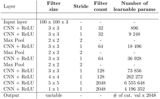
The final architecture with multiple outputs can be seen in the Figure 3.4. For better readability we also provide description of the network in Table 3.1. Including architecture of model we had to settle on numerous specific hyper parameters of each layer, like padding, kernel sizes and kernel counts in convolution layer, pooling layer filter sizes and strides and type of activation function. We opted for rectified linear unit layer as activation function. Also in our model description in figure 3.4 and table 3.1 we do not mention batch normalization layer as we use it as part of convolutional layer and it resides between CNN layer and following activation layer.

From the table 3.1 we can see that the model had in total 11 153 696 trainable parameters without output variables. The output is fully connected

...

Output variable - - # of cat. val x 2048

Table 3.1: CNN model description

layer followed by categorical cross entropy layer. In the fully connected layer we had 2048 parameters times number of categories, so for example for binary attribute like gender we had 4096 parameters. Each convolutional layer had zero padding therefore the these layers also decreased the output resolution compared to the input. We intentionally exploited this property to decrease the number of parameters and speed up processing time.

3. Model description

...

Figure 3.4: The figure shows architecture of the CNN which we used for prediction of attributes from facial images. The figure shows a variant of the CNN predicting 5 attributes.

Chapter

4

Data description

In this chapter we introduce dataset used during testing and development of the model for this thesis.

Our dataset was extracted from CelebA dataset [32] by selecting subset of original categories. Namely gender, glasses, attractiveness, smile and hair color. The first four are binary categories and the the last one have five different classes which are result of merging originally multiple binary labels. The locations of faces in images was extracted by EM-CNN algorithm [42].

Furthermore we examined distributions in our classes and focused on the most ambiguous category which is attractiveness category. Consequently we discovered non negligible bias toward attractive women subcategory in the labeling.

Finally we describe questionnaire created on examples from our CelebA dataset. This questionnaire was used to compare ability to predict labels between our algorithm and humans.

Data split Number of examples Category name Number of categories

Train 162 770 Attractiveness 2

Test 19 962 Glasses 2

Valid. 19 867 Gender 2

Total 202 599 Hair 5

Table 4.1: CelebA dataset overview.

4.1

CelebA dataset

The CelebA dataset was composed of 202 599 pictures. The pictures contained various photographies with face. Each sample was provided with the location of face. The location was defined by bounding box containing four pixel positions in picture. The labeling and bounding boxes were extracted from large scale database[32] with originally just binary labels. For our use case we picked a subset of attributes and the hair category was produced as combination of various original binary labels. The full annotation for our specified version of CelebA dataset contained 5 attribute labels with following categories:

4. Data description

...

Figure 4.1: Examples of CelebA images [32]

.

.

.

.

.

The labels for each sample were provided in separate configuration file. Single line in attributes configuration file contained name of picture followed by encoded values for each attribute in order specified by another configuration file with attribute values. In the attributes values file were at each line category code followed by semantic meaning of label separated by double colon.

Each picture contained picture of face from different angles and in different partition of picture. As locating a face in picture was not our main goal, we were also provided with location parameters of face for each sample so we could crop each sample just to face picture. The location of face in picture was specified in separate configuration file where single line started with name of picture followed by space separated four integer values specifying rectangular frame position of face in picture. Examples of images of before cropping and after can be seen in the section about data augmentation further in text.

After cropping and resizing the original dataset, samples were split into three subsets containing data for training, validating and testing. 80% of

...

the whole dataset was used for training. The remaining 20% of data was equally split between testing and validating subsets. In single epoch data from training sample were used for training and then we evaluated the performance of newly trained parameters on validation data. This evaluation is crucial to be able to spot overfitting of our model. The testing partition was used only once in the final evaluation of network on model from epoch where model achieved the lowest average aggregate validation loss.

4.1.1 Subsets and categories

The training dataset contained 162 770 examples, the validation subset contained 19 962 and the test subset contained 19 867. The distribution of categories in each attribute can be seen on the following graphs and table summarizing all categories. Each category has quite expectable distribution and each data split has approximately same categories distributions.

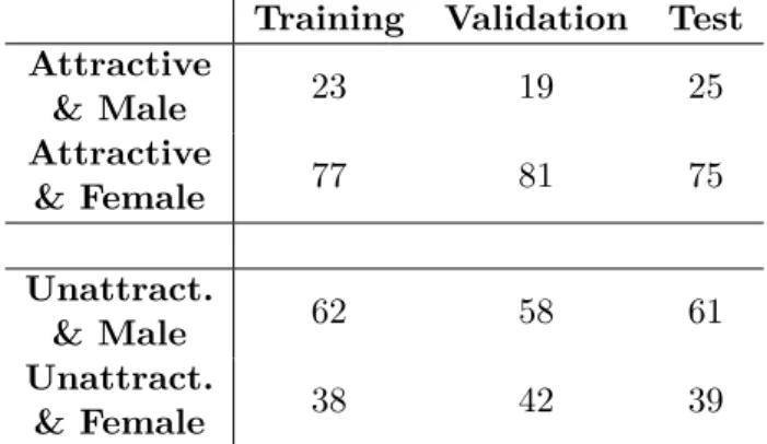
The first category is attractiveness. This class can be one of the most complicated category in dataset as it is very ambiguous category. Specifi-cally there isn’t any well established definition of attractiveness. Moreover attractiveness is highly subjective which is also highly influenced by cultural, personal preferences, geographical location, gender and many more factors concerning the evaluator. Furthermore, it is very unlikely that in creation of this dataset a single evaluator has been used. This introduces another challenge in this class, as it is expected that the values will not have consistent values and it will be even harder to determine intrinsic features responsible for category evaluation. Regarding internal distribution we can observe from the graph a) that we have equal split in attractiveness. However after review of attractiveness class we discovered, that we have non negligible bias toward attractive women. Disparity in the distributions can be detected from the following Table 4.2. As mentioned before it can be due to personal prefer-ences of evaluators of this photographs or that we were able to gather more examples of attractive women celebrities.

Then we have attribute with glasses, where the minority of our population has glasses. In this class, it is important to observe percentage of false negative and false positive errors due to their minor representation. In other words we should oversee the learning process so the classifier would not overfit on examples without glasses and so it would be able to identify occurrence of glasses in examples.

The next attribute category is gender. In this category there are more women than men, which corresponds to natural population and equal split in smile attribute. The last binary category is smile where we have similarly equal split in it values.

From the graph e) we observe unequal distribution of attribute values in hair category. The major value in this attribute is unspecified class with nearly 40%. After reviewing examples from the unspecified class we conclude, that majority of this examples are mixed hair colors which are very equivocal. Specifically there is high number of mixed blond and brown, or some part of color hair was getting gray, yet the gray color was not dominant enough

4. Data description

...

(a) : Distribution in attractiveness class (b) : Distribution in glasses class

(c) : Distribution in gender class (d) : Distribution in smiling class

(e) : Distribution in hair color class

to be marked as gray hair color. Also there were multiple examples with woman who had just partially colored hair as the original color of their hair had already grown out. At last the minority of unspecified color were an extravagant colors like green, purple, etc.

4.2

Questionnaire

For purposes of our thesis we also created small survey with CelebA dataset. This survey contained 100 images from training set. The task for participants was to label each picture with all five categories. We used it to asses the original labeling as the CelebA dataset contained highly subjective category

...

Training Validation Test Attractive & Male 23 19 25 Attractive & Female 77 81 75 Unattract. & Male 62 58 61 Unattract. & Female 38 42 39

Table 4.2: Attractiveness vs. gender in percentage (Rounded)

Split Samples in split

Attractive Glasses Gender Smile Hair color

Yes No Yes No M. F. Yes No Black Blond Brown Gray Other

Train 162 770 51 49 6 94 42 58 48 52 23 14 19 5 39 Valid 19 962 50 50 6 94 39 61 50 50 27 13 17 3 40 Test 19 867 52 48 7 93 43 57 48 52 20 14 23 5 38

Table 4.3: Percentage category distribution per datasets (rounded)

of attractiveness which can be highly specific to cultural preferences. We have to note, that we cannot vouch for statistical correctness of these results as we did not had possibility to randomly approach participants and also we had to made it of considerable size to get at least some answers.

We managed to get 18 respondents to fill out our questionnaire. We firstly compute aggregate human error for each attribute separately. Lets define the true label for the i-th example as li and j-th human evaluation for the i-th

example asevi_j. We useanat as number of present annotations for attribute

at∈ {Attractivenes, Glasses, ...} . Consequently the aggregate human error for single attribute is defined as 1

anat Pp

i

Pn

j[[liat 6= evji[] where n = 100 is number of examples and p = 18 is number of participants. Similarly we

define crowd vote error where the evaluated label for i-th example mvi was

chosen as majority vote from the human evaluation. The crowd vote error was computed as 1

n

Pn

i[[li 6= mvi[]. Results for the survey are presented in the following Table 4.4. We will use these results as one of the baseline error rates for our models and we will abbreviate the metrics as AHC error or just "Human error" for aggregate human correspondent error and CV error for

crowd vote error.

Number of

annotations (AHC) error[%]Aggregate (CV) error [%]Crowd vote

Attractiveness 1795 29.8 28.1

Glasses 1786 1.1 1.0

Gender 1790 1.1 0.9

Smile 1784 15.2 12.9

Hair 1783 50.7 48.3

4. Data description

...

Surprisingly, from this small experiment we can see that our evaluators had struggled the most with hair attribute and secondly with attractiveness attribute. We assume that this is due to ambivalently defined "other" value in the hair attribute. Without proper definition of this value could pose significant challenge for evaluators to distinct between other value and the rest. Moreover after revision of chosen examples it could be also due to similarity of black and brown hair color. On the other hand the higher error rate in attractiveness category was quite expected as the definition of attractiveness can be very distinctive for each human. Given that every evaluator expressed this attribute in his own subjective definition of attractiveness we consider this error reasonable.

Chapter

5

Implementation

In this chapter we describe software and hardware used during implementation. Later we introduce a process of final implementation, training and evaluation of the CNN model. Lastly we introduce additional functionality of our project, such as application of the learned model on video.

5.1

Software

For the implementation we used Python programming language. We have chosen this language as it provides multiple frameworks and libraries to working with neural networks with strong online community support. In python there are many specialized libraries like Caffe, Keras, Tensorflow, Theano, Pythorch and many more. We opted for Keras as it is one of the most frequently used libraries within scientific community[30]. Moreover, as it is a higher level API library, it enables us to use different back-end frameworks and we are not locked in single ecosystem. We used tensorflow as the backend support for Keras. Another advantage of Keras is its simplicity and yet it enables deeper manipulations on back-end level in case of need for further specific functionalities. Also, Keras enables CPU and GPU supported computing. This feature of Keras framework allowed us to easily switch between server sided GPU computing and local CPU debugging without need of complicated configurations.

5.2

Hardware

Main hardware used for learning the network was computing server with CPU E5 2400 and Nvidia GTX Titan Black 6GB graphic card. This GPU has bandwith of 336GB/s which is an important parameter as it caps data inflow for computation. Bigger flow can significantly speed up whole computation. Furthermore, in machine learning, it is crucial to parallelize computation with matrices. GPUs are mainly designed for this kind of computation. The secondary machine for local development and debugging was ultrabook with Intel i5 5200.

5. Implementation

...

For example CPU backed computation on local machine takes 512 mili-seconds for single image forward and backward pass. Comparatively it takes 957 nano-seconds on previously mentioned GPU server.

5.3

Developed framework

In this section we are introducing developed framework for running ex-periments with CNN model. The framework is mainly used for train-ing, testing and evaluation of CNN model which is later utilized in real time multiple face attributes estimation. Basically we will provide the reader with overview of our project which is available at this addresshttps: //gitlab.fel.cvut.cz/marcimat/CNN.git . The project was developed

with goal to support multiple data sources with multiple configuration there-fore majority of its functionality can be influenced with configuration files and its designated readers.

5.3.1 Configuration

The configuration of each database is a bit different, therefore we developed configuration for each database separately with unified output which connects in data generating process. Using object injecting we just use specified loader for data generator and than generator utilizes it to correctly feed data into the model.

Regarding configuration of model architecture everything took place in cnn.py script. Here we specified architecture of our model mentioned in previous chapter. The model was defined through functional KERAS API and was designed to be able to have configurable number of outputs and input resolution of images. In addition this script provided means for serializing and loading of model and its configuration setting, histories produced by training and evaluation of model.

5.3.2 Model development

The development of final model for estimation of multiple attributes went through multiple phases. Disregarding initial steps as choice of framework and choice of programming language the first phase was to create single output CNN architecture.

The reason why we implemented at first just single output architecture was not only to get familiar with framework but also to have some bench mark results. This is crucial as we will have initial values with single output architecture specialized per attribute. Thus it will be easier to compare expressiveness of ensemble of CNN to single network with multiple outputs. We used the same architecture for multiple outputs architecture as in single output scenario with just adjusting the last layer, where in stead of single prediction we will produce multiple.

...

After we settled on initial architecture we had to optimize learning rate. This part is particularly delicate as it is more of craft than straight forward algorithm. The basic behavior of model in the first epochs even batches can hint a lot about properties of chosen learning rate value.

The value of learning rate is too high if the error is increasing with each iteration. Moreover in case the loss hits plateau just after few epochs it indicates also a bit high learning rate. Another problem with very high learning rates is that it can start to over fit quite quickly just after few epochs (approximately 10 - 20). On the other hand if we chose too small values the learning process is slow and the network could reach better results with higher values of learning rate. This behavior of learning rate values is illustrated on the following picture5.1.

Figure 5.1: Behavior of learning rate values[29]

Common practice is to randomly select multiple values from specific interval and then narrow our searching interval based on results. In other words the best learning rates can be found using simulated annealing rather than basic grid search. The whole process of finding right learning rate is quite time consuming process because to correctly asses all aspects of the specific values we had to run at least 25 epochs. Ideally we should run the test with as much epochs as possible. However, regarding that single epoch on our data with lower load on the computation grid server took approximately 14 minutes one test of single learning rate value was nearly six hours. In case of higher load on the server the single epoch computation time could increase up to 20 or even 30 minutes resulting in more than 10 hours per tested value. Consequently our search for optimal learning was strictly limited by the available time and server availability. The optimizer used in our model was previously mentioned Adam optimizer which is currently considered as one of the most versatile and the most balanced optimizer for any neural network application.

5. Implementation

...

Finally we could start training and evaluating our model. Due to limited time we opted to develop as much functionality as possible so we can evaluate our proposed learning model. At last we used our remaining time to tweak our architecture and tried different parameters on previous results.

5.3.3 Mini-batch generation

For feeding data we developed DataGenerator class which responsibility is to correctly load data from disk, pre-process data and sequentially feed model with data for training and evaluation. Due to memory constraints of our hardware we could not feed whole dataset at once into the model, therefore the generator was feeding data in bulks of twelve thousands images.

Firstly the data were fed to KERAS framework as separate arrays for input images and labels extracted from configuration files. Moreover as the CNN model requires uniform picture resolution we had to preprocess each sample. This preprocessing could be done in two manners, on-line or off-line.

The on-line preprocessing means, that each picture would be cropped and resized to specified uniform resolution just in time. The other option, off-line, we prepared our dataset in advance by cropping and resizing before running the network. As training a CNN is highly resource demanding task for computer we opted for the later option of preprocessing during early stages of development and tuning some hyper parameters. Thus the network could be directly fed data from disk without need of any further alteration before inputing into the model. In later stages where we were trying different data augmentation techniques and different input configurations of architecture we switched to on-line data feeding, as it provides better flexibility.

Gradually by adding new functionalities to our framework the baseline generator was used as super object for its descendants like on-line data generator, data generator with ability to hide some label and and augmenting original data and also two other dataset generators.

5.3.4 Data augmentation

Apart from plain data loading we also utilized data augmentation to broaden our training samples. This is done mainly to avoid over fitting on the training set and to increase the ability of the model to generalize. The virtualization process consists of multiple affine transformation of input image. Such changes can be for example mirroring of image or rotation, changing color spectrum and many more. Consequently we can train more general classifier as we provide it with unique images in each training iteration.

In our scenario we are limited to just few possible transformations and we must be careful with parameters. For example we cannot tilt the image to much, definitely not beyond 45 degrees, because identifying facial expression like smile can be made significantly more difficult even for humans, not speaking about algorithms.

Therefore we opted for image mirroring, slight rotation and expansion/retraction of cropping coordinates in such a range that it would not hinder original

...

(a) : Original images (b) : Cropped images by provided face location

(c) : Expanded images (d) : Augmented images Figure 5.2: Images examples

information. The parameters of these augmentations can be seen in table below5.1.

First we randomly expanded/reduce width and height of picture by param-eter from interval <-5,+5>. After that we expanded cropping coordinates by 25% and applied mirroring. The mirroring was randomly assigned to 50% of pictures. Following, we rotated the picture by 0-5 degrees to left of right. At last we scaled the images to final resolution for network. Each parameter value was pseudo randomly generated from mentioned intervals.

For scaling images we used bilinear transformation provided by pillow package. It is important to realize, that mainly the expanding of crop frame can significantly impact performance of the model, therefore we had to apply the 25% expansion of bounding box also to examples used in evaluation and testing phases. It can be seen from examples 5.2 that original bounding boxes are focused on the facial location in images, disregarding hair of person in

5. Implementation

...

the picture. In the set of pictures 5.2b we observe much lesser proportion of hair in comparison to examples 5.2c.

Parameters Rotation +5°, -5° Mirroring 50 % Expanding +5% , -5%

Table 5.1: Virtualization parameters

5.3.5 Final hyper-parameter setting

Training of CNN in its essence is likelihood maximization algorithm where the current configuration is evaluated and updated after each forward pass. The update phase is done by gradient descent which is calculated by back propagation. In the case of partial labeling we have to marginalize over known values before back prop.

However to maximize this update step we have to configure numerous non trainable parameters. This non-trainable parameters are commonly named ad hyper parameters. We used following hyper parameters with values in the brackets:

.

.

.

.

5.4

Live demo

As one of the expected results of this thesis is to use learned model for live demo application. For this we used CV library detection with haar frontal face cascade filter for face detection[31]. This small demo application processed each frame at time. From the frame were identified faces with the haar filter and processed by by our model to estimate attributes from the input image. The identification of faces from the full frame with our detector is highly resource demanding task. Therefore to speed up this process we used facial detection on the full frame only to identify the locations of the faces. Once identified we remembered the locations of those faces. Then we used our detector only to the cropped part of the frame to validate if the face is still present in that location. If the face was not recognized in the original location we rerun the detector on the full frame. This technique significantly decreased processing time for each frame, resulting in better overall performance.

Example of the resulting application of our trained model applied on prediction of face into video is show in the Figure 5.3. However it is important

...

to note, that our model can under perform in predicting attributes from the video as such task is significantly different from the original learning scenario due to constantly changing conditions like luminance, angle of face, resolution etc. Another problem can be in fact that the video frames are creating completely different dataset compared to the training data.

Chapter

6

Experiments

This section covers all experiments that were done using the CelebA dataset. The experiments were conducted in the same order as presented here, as we gradually moved from the single task CNN to multi task model and to learning from partial annotations. The main goals of this chapter is i) to compare single-task and the multi-task CNN prediction models and ii) to compare performance of multi-task CNN models trained either from fully annotated examples or from partially annotated examples. The goal was not to get the state-of-the-art results, but rather to evaluate relative performance of different models and learning scenarios. The main reason for not attempting to beat the state-of-the-art was mainly the limited time we had at our disposal. Nevertheless, as will be seen later the achieved performance is close to the state-of-the-art methods.

6.1

Evaluation protocol

For the sake of comparability, all compared models used the same CNN architecture, up to the output layer defining the predictors, and the learning algorithm used the same hyper-parameters. In particular, for training the CNN model we always used ADAM optimizer running 100 epochs with learning rate 0.000007 and the number of images in the mini-batches was 124.

After finishing the training phase, we had the 100 prediction models each saved at the end of the respective epoch. We selected the best model based on the validation error. In case of training the multi-task CNN model the validation error was computed as the arithmetic average of validation errors of all predicted attributes. We opted for this method rather than taking the last trained model (i.e. at epoch 100), as the neural networks tend to overfit at the end of training stage. In other words, the models from the last epochs often prove to be less general and less accurate on unseen data.

The best model (the one with the minimal validation error) was evaluated on the test examples. As all the attributes are categorical (with small number of values) we used the classification error as the evaluation metric. The classification error was computed as a fraction of test examples on which the value of the predicted and ground-truth attributes disagree.

6. Experiments

...

drawn from statistically independent random variables. In turn we can use the Hoeffding’s inequality [46] to compute the confidence interval for our error estimates. Let ˆR be the test classification error computed froml examples.

By Hoeffding’s inequality, we can claim that the true classification error (i.e. the expected value of the 0/1-loss) is in the interval ( ˆR−ε,Rˆ+ε) with

probability δ= 0.95, where ε= r 1 2l log(2)−log(1−δ) .

In particular, forl= 19,962 test examples the width of the confidence interval

is ε= 0.0096. This means that with probability 95% the true error deviates

from the reported test error by 1% at most.

In our experiments, we compare the multi-task CNN prediction model against several baseline approaches. The main baseline is the single-task CNN model which uses the same architecture as the multi-task CNN but it predicts only a single attribute (there is a single linear classifier on top of the last layer). The additional baseline is a trivial predictor based on random guess of the attribute. The performance of the random predictor sets a pessimistic upper bound on the Bayes error. To get a tight upper bound on the Bayes error, we report the human performance on the same prediction tasks. See Section 4.2 on how the human predictions were collected. Note that humans have been trained during the evolution to recognize the attributes from human faces. Hence, the human performance is often a good approximation of the Bayes error. Last but not least, we also report prediction errors achieved by some state-of-the-art methods on the CelebA dataset.

6.2

Single task model

In this section, we evaluate performance of single task models. For each attribute we trained an independent CNN prediction model which will serve as one of the baselines in the following experiments. In particular, we use the CNN architecture described in Section 3.3, having a single predictor implemented in the output layer. We trained five models, one for each of five attributes, and evaluated the models. Further in text we will refer to this experiment as the single task models (STM).

Firstly, in Table 6.1, we present result summarizing the development stage of our STM model. The table shows training, validation and test error achieved for individual attribute. In addition, we report the number of epochs to get the best model, i.e. the models with the lowest validation error. We can see a small difference between the training and the validation (and test) errors. This relatively small difference hints us that we could increase performance of our model by increasing its complexity, e.g. by increasing depth of the network. Another notable point from the results in Table 6.1 is that the best validation error for attributes with higher error was achieved rather in later training stages as compared to attributes that can be recognized with lower error. More specifically, the best model for the attributes "glasses",

...

"gender" and "smile" was obtained after around thirty training. In contrast, for attributes "attractiveness" and "hair", the best model was achieved after more than fifty epochs. This development can be attributed to intricacy in predicting these attributes or to the inconsistencies in the ground-truth labeling provided with the dataset.

Train Error [%] Test Error [%] Validate Error [%] Best Epoch Attractiveness 17.1 21.4 20.0 55 Glasses 0.6 1.4 1.2 31 Gender 2.5 3.8 4.5 37 Smile 6.5 8.8 9.1 41 Hair 26.4 33.4 33.4 57

Table 6.1: The summary of classification errors obtained in the development stage of the STM model. The table reports the training, validation and the test errors for each predicted attribute. The last column contains the number of training epochs needed to get the model with the smallest validation error.

STM

Error [%]

Error [%]

Random

Human-avg

Error [%]

Human-cv

Error [%]

Attractiveness

21.4

48.0

29.8

28.1

Glasses

1.4

7.0

1.1

1.0

Gender

3.8

42.6

1.1

0.9

Smile

8.8

48.3

15.2

12.9

Hair

33.4

62.4

50.7

48.3

Table 6.2: Comparison of the STM model against the random guess and the human performance. The Human-avg stands for the average human error while Human-cv refers to the prediction based on majority vote of a crowd of humans.

In Table 6.2, we present comparison of the STM model against the random predictor and the human performance. We can clearly observe that our models are significantly better than random guess and furthermore it achieves better results than humans. The STM model did significantly better in prediction of "attractiveness" but also remarkably better in prediction of "hair" color. The disparity in case of the "attractiveness" could be attributed to the fact that the attractiveness is a highly subjective attribute. Hence the humans creating the ground-truth annotation in CelebA database can perceive the attractiveness differently than the humans taking part in our survey. However, the large human error in case of the "hair" color prediction is a bit surprising.

As the CelebA dataset is widely used for benchmarking of face classifica-tion algorithms, we can compare predicclassifica-tion error of our model against the state-of-the-art methods. In particular, we compared against PANDA [41], Facetracer [40], LNets+ANet [39] and DMTL[36]. As our "hair" attribute was

6. Experiments

...

created by joining multiple values from the original database, the comparison of this attribute could be misleading. Therefore we opted to omit it com-pletely and show comparison on four binary attributes only. The results are summarized in Table 6.3. It is seen that the three best performing approaches are DMTL [35], LNet+Anet [39] and the proposed STM which are all based on CNNs. Our method is slightly worst than the best performing method, DMTL [35], but it is better than the LNet+Anet [39]. However, it is impor-tant to note that the DMTL [35] is using more complex architecture which composed of several common layers followed by attribute-specific branch [36]. Our STM model also outperforms the PANDA [41] algorithm and Facetracer which slightly lagged behind the rest.

PANDA[41] Facetracer[40] LNets+ANet[39] DMTL[35] STM

Attractiveness 23 22 19 15 21

Glasses 2 2 1 2 1

Gender 3 9 2 1 4

Smile 8 11 8 6 9

Table 6.3: Comparison of the proposed STM model against state-of-the-art methods PANDA [41], Facetracer [40], LNets+ANet [39] and DMTL [35]. The comparison is carried out on selected binary attributes of the CelebA database.

To conclude, we showed that our STM models have performance similar to the current state-of-the-art methods based on CNNs. In addition, the STM models significantly outperform the human ability to predict the selected attributes. The lower human performance is significant on the attributes whose annotation is very subjective. Based on the results we also identified some possibilities how to improve our model. Namely, the results suggest that making the architecture more complex could further improve the results. Unfortunately, due to lack of time we have not had time to implement these improvements.

6.3

Multiple task model

In this section, we evaluate the multi-task CNN model which uses the archi-tecture described in Section 3.3. Further in the text we will abbreviate this model as MTM standing for multi-tasks model. The architecture of the MTM model is nearly the same as the one used by STM model. The only difference is in the last layer which is, in the case of MTM, composed of multiple linear predictor, one for each attribute. The main goal of the experiment described in this section is to compare performance of the MTM and the STM model. To paraphrase, we wanted to test if the expressiveness of features extracted by the used CNN architecture is sufficient to perform several prediction tasks simulta