Robust deep networks with randomized tensor regression layers
Arinbj¨orn Kolbeinsson
∗Samsung AI, Cambridge
Imperial College London
Jean Kossaifi
∗Samsung AI, Cambridge
Imperial College London
Yannis Panagakis
Samsung AI, Cambridge
Imperial College London
Adrian Bulat
Samsung AI, Cambridge
Anima Anandkumar
California Institute of Technology
Ioanna Tzoulaki
Imperial College London
Paul Matthews
Imperial College London
Abstract
In this paper, we propose a novel randomized tensor de-composition for tensor regression. It allows to stochasti-cally approximate the weights of tensor regression layers by randomly sampling in the low-rank subspace. We the-oretically and empirically establish the link between our proposed stochastic rank-regularization and the dropout on low-rank tensor regression. This acts as an additional stochastic regularization on the regression weight, which, combined with the deterministic regularization imposed by the low-rank constraint, improves both the performance and robustness of neural networks augmented with it. In par-ticular, it makes the model more robust to adversarial at-tacks and random noise, without requiring any adversarial training. We perform thorough study of our method on syn-thetic data, object classification on the CIFAR100 and Ima-geNet datasets, and large scale brain-age prediction on UK Biobank brain MRI dataset. We demonstrate superior per-formance in all cases, as well as significant improvement in robustness to adversarial attacks and random noise.
1. Introduction
Deep neural networks have been evolved to powerful predictive models with remarkable performance on com-puter vision tasks [26, 30,16]. Such models are usually over-parameterized, involving an enormous number (possi-bly millions) of parameters. This is much larger than the typical number of available training samples, making deep networks prone to overfitting [5]. Coupled with overfitting, deep networks lack robustness to small adversarial or noise perturbations [14]. In computer vision tasks, such as image classification or regression, perturbed examples are often
∗Equal contribution
perceived identically to the original ones by humans while lead arbitrarily different predictions by networks. These shortcomings pose a possible obstacle for mass deployment of systems relying on deep learning in sensitive fields such as medical image analysis for disease prediction and expose an inherent weakness in their reliability.
To improve the robustness of deep neural networks to (adversarial or random) perturbations and prevent them from overfitting, several methods that essentially affect the parameters of deep networks via regularization have been investigated. One line of research includes methods that apply regularization functions (e.g., `2- or `1- norm) on
networks parameters [32,27,36,49]. Besides the afore-mentioned general-purpose regularization functions, neural networks specific methods such as early stopping of back-propagation [5], batch normalization [17], dropout [38] and its variants –e.g., DropConnect [44]– are algorithmic ap-proaches to reducing overfitting in over-parametrized net-works and have been widely adopted in practice. An alter-native approach for reducing the number of effective param-eters in deep nets relies on low-rank regularization. That is, by leveraging the redundancy in network parameters, methods such as [41,7,47,23] employ low-rank approx-imations of deep networks weight matrices (or tensors) and hence massively reduce the number of learnable parame-ters. Links between regularization and robustness of deep neural networks to adversarial perturbations have been re-cently established in [2,18].
In this paper, we introduce a novel low-rank inducing regularization method for improving robustness of deep net-works to adversarial and random perturbations. We replace flattening and fully-connected layers entirely with a ran-domized tensor regression layer (R-TRL). This preserves the structure by expressing an output tensor as the result of a tensor contraction between the input tensor and some low-rank regression weight tensors. We propose to obtain
1
the low-rank regression weights by solving a novel random-ized tensor regression model, which leads to the stochastic reduction of the rank, either by a fixed percentage during training or according to a series of Bernoulli random vari-ables. This is akin to dropout, which, by randomly drop-ping units during training, prevents over-fitting. However, rather than dropping random elements from theactivation tensor, this is done on rank of the regression weight tensor. We conduct thorough experiments in image classification and phenotypic trait prediction from MRI analysis. Specif-ically, we apply our method to the UK Biobank brain MRI dataset for estimating brain-age, which has been associated with a range of diseases and mortality [9], and could be an early predictor for Alzheimer’s disease [13]. A more accu-rate and more robust brain age estimation can consequently lead to more accurate disease diagnoses.
In summary, we make the following contributions:
• We propose a novel randomized TRL based on a stochas-tic tensor decomposition
• We explore two schemes: (i) selecting random element to keep in the low-rank subspace, following a Bernoulli distribution and (ii) keeping a random subset of thefibers of the tensor, with replacement.
• We theoretically and empirically establish the link be-tween the proposed randomized TRL and dropout on the deterministic low-rank tensor regression.
• We demonstrate state-of-the-art results for image clas-sification on CIFAR100 and ImageNet, and show supe-rior performance to both the regular network with fully-connected layer and with tensor regression layer without our proposed decomposition.
• Our method makes neural networks significantly more robust to adversarial noise,withoutadversarial training. • We also demonstrate a large performance improvement
(more than 20%) on the regression task using MRI data, with 3D-ResNet and our proposed R-TRL, compared to a regular 3D-ResNet. Our R-TRL is also significantly more robust to random noise in the input.
2. Closely related work
Network regularization and dropout. Several methods that improve generalization by mitigating overfitting have been developed in the context of deep learning. The in-terested reader is referred to the work of [28] and the ref-erences therein for a comprehensive survey of regulariza-tion techniques for deep networks. The most closely re-lated regularization method to our approach is Dropout [38], which is probably the most widely adopted technique for training neural networks while preventing overfitting. Con-cretely, during dropout training each unit (i.e., neuron) is equipped with a binary Bernoulli random variable and only the networks weights whose corresponding Bernoulli vari-ables are sampled with value 1 are updated at each
back-propagation step. At each iteration, those Bernoulli vari-ables are re-sampled again and the weights are updated ac-cordingly. The proposed regularization method can be in-terpreted as dropout on low-rank tensor regression, a fact which we proved in Section4.2.
Randomized tensor decompositions. Tensor decom-positions exhibit high computational cost and low conver-gence rate when applied to massive multi-dimensional data. To accelerate computation, and enable them to scale, ran-domized approaches have been employed. A ranran-domized least squares algorithm for CP decomposition is proposed by [1], which is significantly faster than traditional CP de-composition. In [12], CP is applied on a small tensor generated by multi-linear random projection of the high-dimensional tensor. The CP decomposition of the large-scale tensor is obtained by back projection of the CP de-composition of the small tensor. [46] introduce a fast yet provable randomized CP decomposition that performs ran-domized tensor contraction using FFT. Methods in [37,43] are highly computationally efficient algorithms for comput-ing large-scale CP decompositions by applycomput-ing random pro-jections into a set of small tensors, derived by subdividing a tensor into a set of blocks. Fast randomized algorithms that employ sketching for approximating Tucker decompo-sition have been also investigated [42,50]. More recently, a randomized tensor ring decomposition that employs tensor random projections has been developed in [48]. The most similar method to ours is that of [1], where elements of the tensor are sampled randomly, and each factor of the decom-position updated in an iterative manner. By contrast, our method allows for end-to-end training, and applies random-ization on the fibersof the tensor, effectively randomizing the rank of the weight tensor.
Tensor Regression Layers. Reducing the storage and computational costs of deep networks has become critical for meeting the requirements of environments with limited memory or computational resources. To this end, a surge of network compression and approximation algorithms have recently been proposed in the context of deep learning. By leveraging the redundancy in network parameters, methods such as [41,7,47,23] employ low-rank approximations of deep networks weight matrices (or tensors) for parameter reduction. Network compression methods in the frequency domain [6] have also been investigated. An alternative ap-proach for reducing the number of effective parameters in deep nets relies on sketching, whereby, given a matrix or tensor of input data or parameters, one first compresses it to a much smaller matrix (or tensor) by multiplying it by a (usually) random matrix with certain properties [20,10].
A particularly appealing approach to network compres-sion, especially for visual data (and other types of mul-tidimensional and multi-aspect data), is tensor regression networks [23]. Deep neural networks typically leverage
the spatial structure of input data via series of convolu-tions, point-wise non-linearities, pooling, etc. However, this structure is usually wasted by the addition, at the end of the networks’ architectures, of a flattening layer followed by one or several fully-connected layers. A recent line of study focuses on alleviating this using tensor methods. [22] proposed tensor contraction as a layer, to reduce the size of activation tensors, and demonstrated large space savings by replacing fully-connected layers with this layer. How-ever, a flattening layer and fully-connected layers were still ultimately needed for producing the outputs. Recently, tsor regression networks [23] propose to replace these en-tirely with a tensor regression layer (TRL). This preserves the structure by expressing an output tensor as the result of a tensor contraction between the input tensor and some low-rank regression weight tensors. In addition, these allow for large space savings without sacrificing accuracy. [4] ex-plore the same model with various low-rank structures on the regression weight tensor.
3. Multilinear algebra background
In this section, we introduce the notations and notions necessary to introduce our stochastic rank regularization.
Notation:We denotevvectors (1storder tensors) andM matrices (2ndorder tensors). Idis the identity matrix. We denoteX tensors of orderN ≥ 3, and denote its element (i, j, k)asXi0,i1,···,iN−1 or X(i0, i1,· · ·, iN−1). A colon is used to denote all elements of a mode e.g. the mode-0 fibers ofX are denoted asX:,i1,···,iN−1. The transpose of
Mis denotedM>. Finally, for anyi, j ∈N, i < j,[i . . j]
denotes the set of integers{i, i+1,· · · , j−1, j}, andidivj the integer division ofibyj.
Tensor unfolding: Given a tensor, X ∈
RI0×I1×···×IN−1, its mode-n unfolding is a matrix
X[n] ∈ RIn,IM, withM = Q
N−1
k=0, k6=n
Ik and is defined by the mapping from element(i0, i1,· · ·, iN)to(in, j), with
j=PN−1 k=0, k6=n ik×QN−1 m=k+1, m6=n Im.
Tensor vectorization: Given a tensor, X ∈
RI0×I1×···×IN−1, we can flatten it into a vector vec(X)of size (I0× · · · ×IN−1)defined by the mapping from
ele-ment(i0, i1,· · ·, iN−1)ofX to elementjof vec(X), with
j=PN−1 k=0 ik×Q
N−1
m=k+1Im.
Mode-n product: For a tensorX ∈ RI0×I1×···×IN−1 and a matrixM∈RJ×In, the n-mode product of a tensor is
a tensor of size(I0× · · · ×In−1×J×In+1× · ×IN−1)
and can be expressed using unfolding of X and the classical dot product as: (X ×nM)[n] = MX[n] ∈
RI0×···×In−1×R×In+1×·×IN−1
Generalized inner product: For two
ten-sors X ∈ RK0×···×Kx×I0×···×IN−1 and
Y ∈ RI0×···×IN−1×L0×···×Ly, we denote by
hX,YiN ∈ RK0×···×Kx×IN−1×L0×···×Ly the
contraction of X by W along their N−1 last (respectively first) modes. hX,YiN = PI0 i0=0 PI1 i1=0· · · PIN−1 in=0X···,i0,i1,···,inYi0,i1,···,in,···
Kruskal tensor: Given a tensorX ∈RI0×I1×···×IN−1, the Canonical-Polyadic decomposition (CP), also called PARAFAC, decomposes it into a sum of R rank-1 ten-sors. The number of terms in the sum,R, is known as the rank of the decomposition. Formally, we find the vectors
u(0)k ,u(1)k ,· · ·,u(2)k , fork= [0. . R−1], as well as an op-tional vector of weightsλ∈RRto absorbs the magnitude
of the factors such that: X = R−1 X k=0 λku(0)k ◦u(1)k ◦ · · · ◦u(kN−1) | {z } rank-1 components , (1)
For any k ∈ [0 . . N−1], these vectors u(rk), r ∈ [0 . . R−1] can be collected in matrices, called fac-tors or the decomposition, and defined as U(k) =
h
u(0k),u1(k),· · · ,u(Rk−)1
i .
The decomposition can be denoted more com-pactly as X = JU(0),· · ·,U(N−1)
K, or X =
Jλ;U
(0),· · · ,U(N−1)
Kif a weights vector is used.
Tucker tensor: Given a tensorX ∈ RI0×I1×···×IN−1, we can decompose it into a low rank core G ∈
RR0×R1×···×RN−1 by projecting along each of its modes with projection factors U(0),· · · ,U(N−1)
, withU(k) ∈
RRk,Ik, k∈(0,· · · , N−1). The tensor in its decomposed
form can then be written:
X =G ×0U(0)×1U(2)× · · · ×N−1U(N−1) =JG;U(0),· · ·,U(N−1)K (2) Note that the Kruskal form of a tensor can be seen as a Tucker tensor with a super-diagonal core.
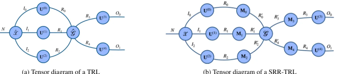
Tensor diagrams:In order to represent easily tensor op-erations, we adopt the tensor diagrams, where tensors are represented by vertices (circles) and edges represent their modes. The degree of a vertex then represents its order. Connecting two edges symbolizes a tensor contraction be-tween the two represented modes. Figure1presents a ten-sor diagram of the tenten-sor regression layer and its stochastic rank-regularized counter-part.
4. Randomized tensor regression layer
In this section, we introduce the randomized tensor re-gression layer. Specifically, we propose a new stochastic rank-regularization, applied to low-rank tensors in decom-posed forms. This formulation is general and can be applied to any type of decomposition. We introduce it here, without loss of generality, to the case of Tucker and CP decomposi-tions.
̂𝒢 U(0) U(1) U(2) U(3) U(4) ̂𝒳 I0 I1 I2 N O0 O1 R0 R1 R2 R3 R4
(a) Tensor diagram of a TRL (b) Tensor diagram of a SRR-TRL
Figure 1: Tensor diagrams of the TRL (left) and our proposed SRR-TRL (right), with low-rank constraints imposed on the regression weights tensor using a Tucker decomposition. Note that the CP case is readily given by this formulation by additionally having the core tensorGbe super-diagonal, and settingM=M(0)=· · ·=M(N)= diag(λ).
Tensor regression layer Let us denote by X ∈
RI0×I1×···×IN−1 the input activation tensor for a sample
andy ∈ RIN the label vector. A tensor regression layer
estimates the regression weight tensorW ∈RI0×I1×···×IN,
expressed under some low-rank decomposition.
For instance, if a Tucker decomposition with rank (R0,· · ·, RN)is used, we have: y=hX,WiN+b withW=G ×0U(0)×1U(1)· · · ×NU(N) (3) with G ∈ RR0×···×RN, U(k) ∈ RIk×Rk for each k in [0. . N]andU(N)∈ RO×RN.
A new randomized tensor decomposition We pro-pose a novel randomized decomposition on W: for any k ∈ [0 . . N], let M(k) ∈
RR0×R0 be a sketch matrix
(e.g. a random projection or column selection matrix) and,
˜
U(k) = U(k)(M(k))> be a sketch of factor matrixU(k), andG˜= G ×0M(0)× · · · ×N M(N)a sketch of the core tensorG.
We can now express our Randomized-Tensor Regres-sion Layer (R-TRL). Given an activation tensor X ∈
RI0×···×IN−1 and a target label vectory ∈
RIN, a R-TRL
layer is written from equation3as follows:
y=hX,Wi˜ N−1 (4)
withW˜ being a stochastic approximation of Tucker de-composition, namely:
˜
W= ˜G ×0U˜(0)× · · · ×N U˜(N) (5) Even though several sketching methods have been pro-posed, we focus here on SRR with two different types of binary sketching matrices, namely binary matrix sketching with replacement and binary diagonal matrix sketching with Bernoulli entries, which we detail below.
4.1. R-TRL with replacement:
In this setting, we introduce the SRR with binary sketch-ing matrix (with replacement). We first chooseθ∈[0,1].
Mathematically, we introduce the uniform sampling ma-trices M(0) ∈
RR0×R0,· · ·,M(N) ∈ RRN×RN. Mj is a uniform sampling matrix, selecting Kj elements, where Kj =Rjdivθ. In other words, for anyi∈[0. . N],M(i)
verifies: M(i)(j,:) = ( 0 ifj > K Idm(r,:), m∈[0. . Ri] otherwise (6)
Note that in practice this product is never explicitly com-puted, we simply select the correct elements fromGand its corresponding factors.
4.2. R-TRL with Bernoulli sampling
In this setting, we introduce the SRR with diagonal bi-nary sketching matrix with Bernoulli entries.
Bernoulli Tucker randomized tensor regression For any n ∈ [0 . . N], let λ(n) ∈
RRn be a random vec-tor, the entries of which are i.i.d. Bernoulli(θ), then a di-agonal Bernoulli sketching matrix is defined as M(n) =
diag(λ(n)).
When the low-rank structure on the weight tensorW˜ of the TRL is imposed using a Tucker decomposition, the ran-domized Tucker approximation is expressed as:
˜ W=G ×0M(0)× · · · ×N+1M(N) ×0 U(0)(M(0))>× · · · ×N+1 U(N)(M(N))> =JG˜;U˜(0),· · ·,U˜(N)K (7) The main advantage of considering the above-mentioned sampling matrices is that the products
˜
U(k)=U(k)(M(k))>orG˜=G ×0M(0)× · · · ×
N M(N) are never explicitly computed, we simply select the elements fromGand the corresponding factors.
Interestingly, in analogy to dropout, where each hidden unit is dropped independently with probability1−θ, in the
proposed randomized tensor decomposition, the columns of the factor matrices and the corresponding fibers of the core tensor are dropped independently and consequently therank of the tensor decomposition is stochastically dropped.
Bernoulli CP randomized tensor regression An inter-esting special case of5is when the weight tensorW˜ of the TRL is expressed using a CP decomposition. In that case, we setM = M(0) = · · · =M(N) = diag(λ), with, for
anyk∈[0. . R],λk ∼Bernoulli(θ).
Then a randomized CP approximation is expressed as: ˜ W= R−1 X k=0 ˜ U(0)k ◦ · · · ◦U˜(N) k (8)
The above randomized CP decomposition on the weights is equivalent to the following formulation:
˜ W= R−1 X k=0 λkU(0)k ◦ · · · ◦U(0)N =Jλ; U(0),· · ·,U(N)K (9)
This is easy to see by looking at the individual ele-ments of the sketched factors. Let k ∈ [0 . . N] and ik ∈ [0 . . Ik], r ∈ [0 . . R−1]. Then U˜ (k) ik,r = PR−1 j=0 U (k)
ik,jMj,r. Since M = diag(λ), i.e. ∀i, j ∈ [0 . . R−1],Mij = 0 if i 6= j, and λi otherwise, we get U˜(ik) k,r = λrU (k) ik,r. It follows that ˜ Wi0,i1,···,iN = PR−1 r=0 λkU (0) k ◦ · · · ◦λkU (N) k .Sinceλr∈ {0,1},we have ˜ Wi0,i1,···,iN = PR−1 r=0 λk U(0)k ◦ · · · ◦U(kN).
Based on the previous stochastic regularization, for an activation tensorX and a corresponding label vectory, the optimization problem for our tensor regression layer with stochastic regularization is given by:
min U(0),···,U(N)k y−1 θhJλ;U (0), · · · ,U(N)K,X iN−1k2F (10) In addition, the above stochastic optimization problem can be rewritten as a deterministic regularized problem:
Eλ min U(0),···,U(N) ky−1 θhJλ;U (0),· · ·,U(N) K,X iN−1k 2 F = min U(0),···,U(N) ky− hJU (0),· · ·,U(N) K,X iN−1k 2 F + 1−θ θ R−1 X k=0 N Y i=0 kU(:i,k) ! k2 2 (11)
This is easy to see by considering the equivalent rewrit-ing of the above optimization problem, usrewrit-ing the mode-N unfolding of the weight tensor. Equation10then becomes:
min U(0),···,U(N)ky− 1 θU (N)diag(λ)(U(−N))>vec(X)k2 F
withU(−N) = U(0) · · · U(N).The result can then be obtained following [31, Lemma A.1].
5. Experimental evaluation
In this section, we introduce the experimental setting, databases used, and implementation details. We experi-mented on several datasets, across various tasks, namely im-age classification and MRI-based regression. All methods were implemented∗using PyTorch [33] and TensorLy [24].
5.1. Numerical experiments on synthetic data
Here, we empirically demonstrate the equivalence be-tween our stochastic rank regularization and the determin-istic regularization based formulation of the dropout.
To do so, we first created a random regression weight tensorWto be a third order tensor of size(25×25×25), formed as a low-rank Kruskal tensor with15components, the factors of which were sampled from an i.i.d. Gaussian distribution. We then generated a tensor of10000random samples,X of size(10000×25×25×25), the elements of which were sampled from a Normal distribution. Finally, we constructed the corresponding response arrayyof size 10000 as: ∀i ∈ [1 . . 1500],yi = hXi,Wi. Using the same regression weight tensor and same procedure, we also generated1000testing samples and labels.
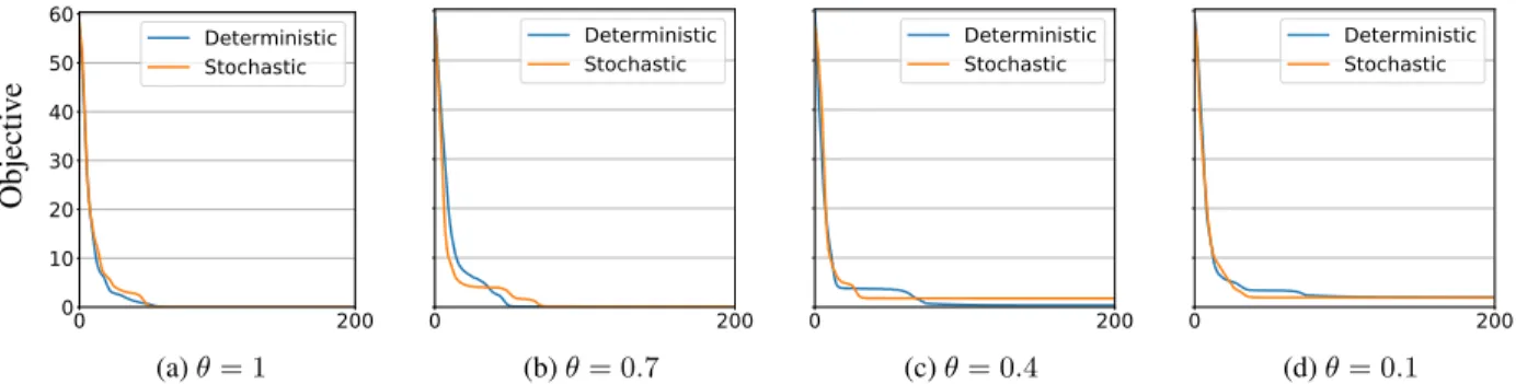
We use this data to train a rank-15CP R-TRL, with both our Bernoulli stochastic formulation (equation 10) and its deterministic counter-part (equation 11). We train for500 epochs, with a batch-size of200, and an initial learning rate of10e−4, which we decrease by a factor of10every200 epochs. Figure2shows the loss function as a function of the epoch number. As expected, both formulations are identi-cal.
5.2. Results on image classification
In the image classification setting, we perform a thor-ough study of our method on the CIFAR100 dataset. In particular, we empirically compare our approach to both standard baseline and traditional tensor regression, and as-sess the robustness of each method in the face of adversarial noise. We also report results for large-scale image classifi-cation on the ImageNet dataset.
CIFAR-100 [25]consists of 60,00032×32RGB images in 100 classes, divided into50,000images for training and 10,000for testing. We pre-processed the data by centering and scaling each image and then augmented the training im-ages with random cropping and random horizontal flipping. We compare the randomized tensor regression layer to full-rank tensor regression, average pooling and a fully-connected layer in an 18-layer residual network (ResNet) [16]. For all networks, we used a batch size of 128 and
Objecti v e 0 200 0 10 20 30 40 50 60 Deterministic Stochastic (a)θ= 1 0 200 Deterministic Stochastic (b)θ= 0.7 0 200 Deterministic Stochastic (c)θ= 0.4 0 200 Deterministic Stochastic (d)θ= 0.1
Figure 2: Experiment on synthetic data:loss of the R-TRL as a function of the number of epochs for the stochastic version (orange) and the deterministic one based on the regularized objective function (blue). As expected, both formulations are empirically the same.
trained for 400 epochs, and minimized the cross-entropy loss using stochastic gradient descent (SGD). The initial learning rate was set to0.01and lowered by a factor of10 at epochs150,250and350. We used a weight decay (L2
penalty) of10−4and a momentum of0.9.
ImageNet [11]is a large-scale dataset for image classifi-cation composed of1.2million training images and50,000 images for validation. We evaluate the classification er-ror in terms of top-1 and top-5 classification accuracy on a224×224single center crop from the raw input images. For training, we use a ResNet101 and follow the same pro-cedure and setting as [16,23].
ResultsTable1presents results obtained on the CIFAR-100 dataset, on which our method matches or outperforms other methods, including the same architectures without R-TRL. Our regularization method makes the network more robust by reducing over-fitting, thus allowing for superior performance on the testing set.
ResNet classification Accuracy
FC 75.88 % FC + dropout 75.84 % Tucker 76.02 % CP 75.77 % Randomized Tucker 76.05 % Randomized CP 76.19%
Table 1: Classification accuracy for CIFAR-100with a ResNet and various regression layers for classification.
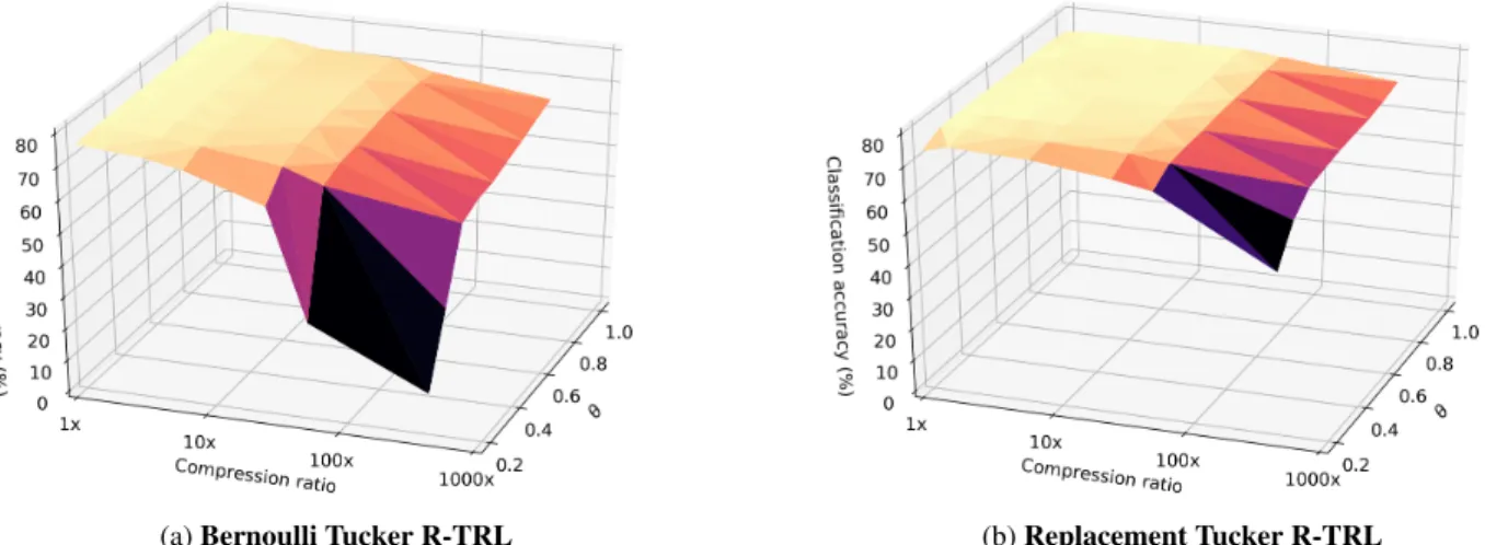
A natural question is whether the model is sensitive to the choice of rank andθ(or drop rate when sampling with repetition). To assess this, we show the performance as a function of both rank andθin figure3. As can be observed, there is a large surface for which performance remains the same while decreasing both parameters (note the logarith-mic scale for the rank). This means that, in practice, choos-ing good values for these is not a problem.
We also test method on the more challenging ImageNet dataset. The results, Table 2 show that our method out-performs the baselines, with higher classification accuracy even for large values ofθ.
Robustness to adversarial attacks: We test for robust-ness to adversarial examples produced using the Fast Gra-dient Sign Method [29] in Foolbox [35]. In this method, the sign of the optimization gradient multiplied by the pertur-bation magnitude is added to the image in a single iteration. The perturbations we used are of magnitudesλ×10−3, λ∈
{1,2,4,8,16,32,64,128}.
In addition to improving performance by reducing over-fitting, our proposed stochastic regularization makes the model more robust to perturbations in the input, for both random noise and adversarial attacks.
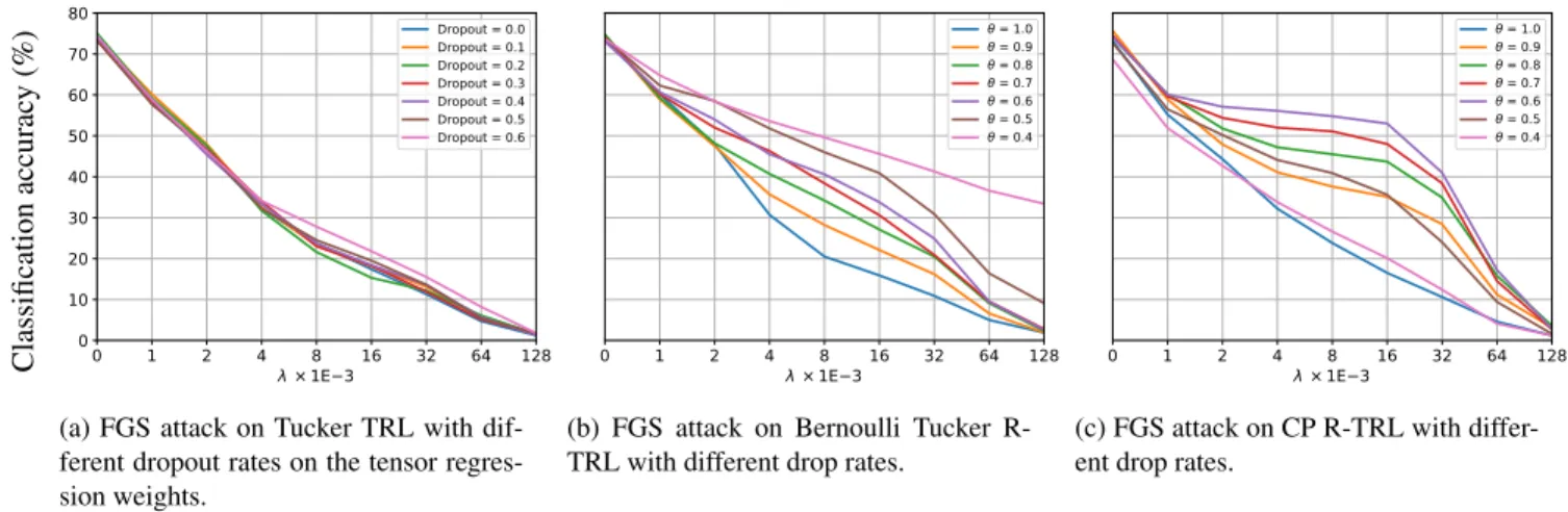
We tested the robustness of our models to adversarial at-tacks, when trained in the same configuration. In figure4, we report the classification accuracy on the test set, as a function of the added adversarial noise. Specifically, we sample1,000images from the test set [3]. The models were trainedwithoutany adversarial training, on the training set, and adversarial noise was added to the test samples using the Fast Gradient Sign method. Our model is much more ro-bust to adversarial attacks. Finally, we perform a thorough comparison of the various regularization strategies, the re-sults of which can be seen in figure5.
We perform a similar experiment on ImageNet (Fig-ure6), using Tucker R-TRL with half the full-rank and ar-rive at similar conclusion.
5.3. Phenotypic trait prediction from MRI data
In the regression setting, we investigate the performance of our R-TRL in a challenging, real-life application on a very large-scale dataset. This case is particularly interest-ing since MRI volumes are large 3D tensors, all modes of which carry important information. The spatial informa-tion is tradiinforma-tionally discarded during the flattening process, which we avoid by using a tensor regression layer.
(a)Bernoulli Tucker R-TRL (b)Replacement Tucker R-TRL
Figure 3:CIFAR-100 test accuracyas a function of the compression ratio (logarithmic scale) and the Bernoulli probability θ(left) or the drop rate (right). There is a large region for which dropping both the rank andθdoes not hurt performance.
Classification accurac y (%) 0 1 2 4 8 16 32 64 128 × 1E 3 0 10 20 30 40 50 60 70 80 FC FC + Dropout = 0.6 CP R-TRL, = 0.6 Tucker R-TRL, = 0.6
Figure 4:Robustness to adversarial attacks on CIFAR100 us-ing Fast Gradient Sign attacks of various models. Our ran-domized TRL architecture is much more robust to adversar-ial attacks, even though adversaradversar-ial training was not used.
Accuracy Model θ Top-1(%) Top-5(%) ResNet 7 77.1 93.4 Ours 0.9 77.7 93.7 Ours 0.8 77.7 93.7 Ours 0.7 77.4 93.6 Ours 0.6 78.0 93.8
Table 2: Classification accuracy on ImageNet with Bernoulli Tucker R-TRL.
The UK Biobank brain MRI dataset is the world’s largest MRI imaging database of its kind [39]. The aim of the UK Biobank Imaging Study is to capture MRI scans of vital organs for100,000primarily healthy individuals by
2022. Associations between these images and lifestyle fac-tors and health outcomes, both of which are already avail-able in the UK Biobank, will enavail-able researchers to improve diagnoses and treatments for numerous diseases. The data we use here consists of T1-weighted182×218×182MR images of the brain for 7,500individuals captured on a 3 T Siemens Skyra system. 5,700are used for training,800 are used for validation and1,000samples are used to test. The target label is the age for each individual at the time of MRI capture. We use skull-stripped images that have been aligned to the MNI152 template [19] for head-size normal-ization. We then center and scale each image to zero mean and unit variance for intensity normalization.
Architecture Regression MAE
3D-ResNet FC 3.23 years
3D-ResNet Tucker 2.99 years
Ours Randomized Tucker 2.77 years Ours Randomized CP 2.58 years
Table 3: Classification accuracy for UK Biobank MRI.
The ResNet models with R-TRL performs significantly out-performs the version with a fully-connected (FC) layer.
Results: For MRI-based experiments we implement an 18-layer ResNet with three-dimensional convolutions. We minimize the mean squared error using Adam [21], starting with an initial learning rate of 10−4, reduced by a factor
of 10 at epochs 25, 50, and 75. We train for 100 epochs with a mini-batch size of 8 and a weight decay (L2penalty)
of 5×10⁻⁴. For Tucker-based R-TRL we used a tensor
with rank128×6×7×6. For CP-based R-TRL we used a Kruskal tensor with 82components. As previously
ob-Classification accurac y (%) 0 1 2 4 8 16 32 64 128 × 1E 3 0 10 20 30 40 50 60 70 80 Dropout = 0.0 Dropout = 0.1 Dropout = 0.2 Dropout = 0.3 Dropout = 0.4 Dropout = 0.5 Dropout = 0.6
(a) FGS attack on Tucker TRL with dif-ferent dropout rates on the tensor regres-sion weights. 0 1 2 4 8 16 32 64 128 × 1E 3 0 10 20 30 40 50 60 70 80 = 1.0 = 0.9 = 0.8 = 0.7 = 0.6 = 0.5 = 0.4
(b) FGS attack on Bernoulli Tucker R-TRL with different drop rates.
0 1 2 4 8 16 32 64 128 × 1E 3 0 10 20 30 40 50 60 70 80 = 1.0 = 0.9 = 0.8 = 0.7 = 0.6 = 0.5 = 0.4
(c) FGS attack on CP R-TRL with differ-ent drop rates.
Figure 5: Robustness to adversarial attacks, measured by adding adversarial noise to the test images, using the Fast Gradient Sign, on CIFAR-100 and Bernoulli drop. We compare a Tucker tensor regression layer with dropout applied to the regression weight tensor5ato our randomized TRL, both in the Tucker (Subfig.5b) and CP (Subfig.5c) case.
Classification accurac y (%) 0 1 2 4 8 16 32 64 128 × 1E 3 0 10 20 30 40 50 60 70 80 = 0.6 = 0.7 = 0.8 = 0.9 FC
Figure 6:Robustness to adversarial attacks on ImageNet. Our R-TRL architecture is much more robust to adversarial at-tacks, even though adversarial training was not used. served, our randomized tensor regression network outper-forms the ResNet baseline by a large margin, Table3. To put this into context, the current state-of-art for convolu-tional neural networks on age prediction from brain MRI on most datasets is an MAE of around 3.6 years [8].
Robustness to noise: We tested the robustness of our model to white Gaussian noise added to the MRI data. Noise in MRI data typically follows a Rician distribu-tion but can be approximated by a Gaussian for signal-to-noise ratios (SNR) greater than2[15]. As both the signal (MRI voxel intensities) and noise are zero-mean, we define
SNR = σ
2 signal σ2
noise
, whereσis the variance. We incrementally increase the added noise in the test set and compare the error rate of the models.
The ResNet with R-TRL is significantly more robust to added white Gaussian noise compared to the same
architec-100.0 25.0 11.1 6.2 4.0 2.8 2.0 1.6 1.2 1.0
Signal-to-noise ratio
0
2
4
6
8
10
12
14
Mean absolute error (years)
3D-ResNet
3D-ResNet with Tucker TRL Ours - Tucker R-TRL
Figure 7: Age prediction error on the MRI test setas a function of increased added Gaussian noise. Shaded regions indicate95%confidence intervals for5independent runs.
tures without it (figure 7). At signal-to-noise ratios below 10, the accuracy of a standard fully-connected ResNet is worse than a naive model that predicts the mean of train-ing set (MAE = 7.9 years). Brain morphology is an im-portant attribute that has been associated with various bio-logical traits including cognitive function and overall health [34,40]. By keeping the structure of the brain represented in MRI in every layer of the architecture, the model has more information to learn a more accurate representation of the entire input. Randomly dropping the rank forces the repre-sentation to be robust to confounds. This a particularly im-portant property for MRI analysis since intensities and noise artifacts can vary significantly between MRI scanners [45]. Randomized tensor regression layers enable both more ac-curate and more robust trait predictions from MRI that can consequently lead to more accurate disease diagnoses.
6. Conclusion
We introduced a novel randomized tensor decomposi-tion, suitable for end-to-end training of tensor regression layer. By adding stochasticity on the rank during training, it renders the network more robust and lead to better perfor-mance. This results in networks that are more resilient to noise, both adversarial and random, without any adversarial training. Our results demonstrate superior performance on a variety of real-life, large scale challenging tasks, including MRI data and images, as well as much better robustness to noise. Finally, we also prove the link between this random-ized TRL and dropout on the deterministic version.
Acknowledgements
This research has been conducted using the UK Biobank Resource under Application Number 18545.
References
[1] C. Battaglino, G. Ballard, and T. G. Kolda. A practical
ran-domized cp tensor decomposition. SIAM Journal on Matrix
Analysis and Applications, 39(2):876–901, 2018.2
[2] A. Bietti, G. Mialon, D. Chen, and J. Mairal. A kernel
per-spective for regularizing deep neural networks. 2019.1
[3] W. Brendel, J. Rauber, and M. Bethge. Decision-based ad-versarial attacks: Reliable attacks against black-box machine
learning models.arXiv preprint arXiv:1712.04248, 2017.6
[4] X. Cao, G. Rabusseau, and J. Pineau. Tensor regression
net-works with various low-rank tensor approximations. CoRR,
abs/1712.09520, 2017.3
[5] R. Caruana, S. Lawrence, and C. L. Giles. Overfitting in neural nets: Backpropagation, conjugate gradient, and early
stopping. InAdvances in neural information processing
sys-tems, pages 402–408, 2001.1
[6] W. Chen, J. Wilson, S. Tyree, K. Q. Weinberger, and Y. Chen. Compressing convolutional neural networks in the frequency
domain. InProceedings of the 22nd ACM SIGKDD
Interna-tional Conference on Knowledge Discovery and Data
Min-ing, pages 1475–1484. ACM, 2016.2
[7] Y. Cheng, F. X. Yu, R. S. Feris, S. Kumar, A. Choudhary, and S.-F. Chang. An exploration of parameter redundancy
in deep networks with circulant projections. InProceedings
of the IEEE International Conference on Computer Vision,
pages 2857–2865, 2015.1,2
[8] J. H. Cole, R. P. Poudel, D. Tsagkrasoulis, M. W. Caan, C. Steves, T. D. Spector, and G. Montana. Predicting brain age with deep learning from raw imaging data results in a
re-liable and heritable biomarker. NeuroImage, 163:115–124,
2017.8
[9] J. H. Cole, S. J. Ritchie, M. E. Bastin, M. V. Hern´andez, S. M. Maniega, N. Royle, J. Corley, A. Pattie, S. E. Harris,
Q. Zhang, et al. Brain age predicts mortality. Molecular
psychiatry, 2017.2
[10] A. Daniely, N. Lazic, Y. Singer, and K. Talwar.
Sketch-ing and neural networks. arXiv preprint arXiv:1604.05753,
2016.2
[11] J. Deng, W. Dong, R. Socher, L.-J. Li, K. Li, and L. Fei-Fei. Imagenet: A large-scale hierarchical image database. In
CVPR, 2009.6
[12] N. B. Erichson, K. Manohar, S. L. Brunton, and J. N.
Kutz. Randomized cp tensor decomposition. arXiv preprint
arXiv:1703.09074, 2017.2
[13] K. Franke, E. Luders, A. May, M. Wilke, and C. Gaser. Brain maturation: predicting individual brainage in children and
adolescents using structural mri. Neuroimage, 63(3):1305–
1312, 2012.2
[14] I. J. Goodfellow, J. Shlens, and C. Szegedy.
Explain-ing and harnessExplain-ing adversarial examples. arXiv preprint
arXiv:1412.6572, 2014.1
[15] H. Gudbjartsson and S. Patz. The rician distribution of noisy
mri data. Magnetic resonance in medicine, 34(6):910–914,
1995.8
[16] K. He, X. Zhang, S. Ren, and J. Sun. Deep residual
learn-ing for image recognition. InProceedings of the IEEE
con-ference on computer vision and pattern recognition, pages
770–778, 2016.1,5,6
[17] S. Ioffe and C. Szegedy. Batch normalization: Accelerating deep network training by reducing internal covariate shift.
arXiv preprint arXiv:1502.03167, 2015.1
[18] D. Jakubovitz and R. Giryes. Improving dnn robustness to
adversarial attacks using jacobian regularization. In
Pro-ceedings of the European Conference on Computer Vision (ECCV), pages 514–529, 2018.1
[19] M. Jenkinson, P. Bannister, M. Brady, and S. Smith. Im-proved optimization for the robust and accurate linear
regis-tration and motion correction of brain images. Neuroimage,
17(2):825–841, 2002.7
[20] S. P. Kasiviswanathan, N. Narodytska, and H. Jin. Deep
neural network approximation using tensor sketching.arXiv
preprint arXiv:1710.07850, 2017.2
[21] D. P. Kingma and J. Ba. Adam: A method for stochastic
optimization.arXiv preprint arXiv:1412.6980, 2014.7
[22] J. Kossaifi, A. Khanna, Z. Lipton, T. Furlanello, and
A. Anandkumar. Tensor contraction layers for
parsimo-nious deep nets. InComputer Vision and Pattern
Recogni-tion Workshops (CVPRW), 2017 IEEE Conference on, pages
1940–1946. IEEE, 2017.3
[23] J. Kossaifi, Z. C. Lipton, A. Khanna, T. Furlanello, and
A. Anandkumar. Tensor regression networks. CoRR,
abs/1707.08308, 2018.1,2,3,6
[24] J. Kossaifi, Y. Panagakis, and M. Pantic. Tensorly: Tensor
learning in python. arXiv preprint arXiv:1610.09555, 2016.
5
[25] A. Krizhevsky and G. Hinton. Learning multiple layers of features from tiny images. Technical report, Citeseer, 2009.
5
[26] A. Krizhevsky, I. Sutskever, and G. E. Hinton. Imagenet classification with deep convolutional neural networks. In
NIPS, 2012.1
[27] A. Krogh and J. A. Hertz. A simple weight decay can
im-prove generalization. InAdvances in neural information
[28] J. Kukaˇcka, V. Golkov, and D. Cremers.
Regulariza-tion for deep learning: A taxonomy. arXiv preprint
arXiv:1710.10686, 2017.2
[29] A. Kurakin, I. Goodfellow, and S. Bengio. Adversarial
exam-ples in the physical world.arXiv preprint arXiv:1607.02533,
2016.6
[30] Y. LeCun, Y. Bengio, and G. Hinton. Deep learning.nature,
521(7553):436, 2015.1
[31] P. Mianjy, R. Arora, and R. Vidal. On the implicit bias
of dropout. In J. Dy and A. Krause, editors,International
Conference on Machine Learning (ICML), volume 80 of
Proceedings of Machine Learning Research, pages 3540– 3548, Stockholmsmssan, Stockholm Sweden, 10–15 Jul
2018. PMLR.5
[32] S. J. Nowlan and G. E. Hinton. Simplifying neural networks
by soft weight-sharing. Neural computation, 4(4):473–493,
1992.1
[33] A. Paszke, S. Gross, S. Chintala, G. Chanan, E. Yang, Z. De-Vito, Z. Lin, A. Desmaison, L. Antiga, and A. Lerer.
Auto-matic differentiation in pytorch. 2017.5
[34] A. Pfefferbaum, D. H. Mathalon, E. V. Sullivan, J. M. Rawles, R. B. Zipursky, and K. O. Lim. A quantitative mag-netic resonance imaging study of changes in brain
morphol-ogy from infancy to late adulthood. Archives of neurology,
51(9):874–887, 1994.8
[35] J. Rauber, W. Brendel, and M. Bethge. Foolbox: a python toolbox to benchmark the robustness of machine learning
models (2017).URL http://arxiv. org/abs/1707.04131, 2017.
6
[36] S. Scardapane, D. Comminiello, A. Hussain, and A. Uncini.
Group sparse regularization for deep neural networks.
Neu-rocomputing, 241:81–89, 2017.1
[37] N. D. Sidiropoulos, E. E. Papalexakis, and C. Faloutsos. Pallel randomly compressed cubes: A scalable distributed
ar-chitecture for big tensor decomposition. IEEE Signal
Pro-cessing Magazine, 31(5):57–70, 2014.2
[38] N. Srivastava, G. Hinton, A. Krizhevsky, I. Sutskever, and R. Salakhutdinov. Dropout: a simple way to prevent neural
networks from overfitting.The Journal of Machine Learning
Research, 15(1):1929–1958, 2014.1,2
[39] C. Sudlow, J. Gallacher, N. Allen, V. Beral, P. Burton, J. Danesh, P. Downey, P. Elliott, J. Green, M. Landray, et al. Uk biobank: an open access resource for identifying the causes of a wide range of complex diseases of middle and
old age.PLoS medicine, 12(3):e1001779, 2015.7
[40] G. E. Swan, C. DeCarli, B. Miller, T. Reed, P. Wolf, L. Jack, and D. Carmelli. Association of midlife blood pressure to
late-life cognitive decline and brain morphology.Neurology,
51(4):986–993, 1998.8
[41] C. Tai, T. Xiao, Y. Zhang, X. Wang, et al. Convolutional
neural networks with low-rank regularization.arXiv preprint
arXiv:1511.06067, 2015.1,2
[42] C. E. Tsourakakis. Mach: Fast randomized tensor
decom-positions. InProceedings of the 2010 SIAM International
Conference on Data Mining, pages 689–700. SIAM, 2010.2
[43] N. Vervliet, O. Debals, L. Sorber, and L. De Lathauwer. Breaking the curse of dimensionality using decompositions
of incomplete tensors: Tensor-based scientific computing
in big data analysis. IEEE Signal Processing Magazine,
31(5):71–79, 2014.2
[44] L. Wan, M. Zeiler, S. Zhang, Y. Le Cun, and R. Fergus.
Reg-ularization of neural networks using dropconnect. In
Interna-tional Conference on Machine Learning, pages 1058–1066,
2013.1
[45] L. Wang, H.-M. Lai, G. J. Barker, D. H. Miller, and P. S. Tofts. Correction for variations in mri scanner sensitivity in
brain studies with histogram matching. Magnetic resonance
in medicine, 39(2):322–327, 1998.8
[46] Y. Wang, H.-Y. Tung, A. J. Smola, and A. Anandkumar. Fast and guaranteed tensor decomposition via sketching. In C. Cortes, N. D. Lawrence, D. D. Lee, M. Sugiyama, and
R. Garnett, editors,Advances in Neural Information
Process-ing Systems (NIPS), pages 991–999. 2015.2
[47] X. Yu, T. Liu, X. Wang, and D. Tao. On compressing deep
models by low rank and sparse decomposition. In 2017
IEEE Conference on Computer Vision and Pattern Recog-nition (CVPR), pages 67–76. IEEE, 2017.1,2
[48] L. Yuan, C. Li, J. Cao, and Q. Zhao. Randomized tensor ring decomposition and its application to large-scale data
recon-struction.arXiv preprint arXiv:1901.01652, 2019.2
[49] Y. Zhang, J. D. Lee, and M. I. Jordan. l1-regularized neural networks are improperly learnable in polynomial time. In
International Conference on Machine Learning, pages 993–
1001, 2016.1
[50] G. Zhou, A. Cichocki, and S. Xie. Decomposition of
big tensors with low multilinear rank. arXiv preprint