The Author(s)BMC Systems Biology2016,10(Suppl 3):68 DOI 10.1186/s12918-016-0312-1
R E S E A R C H
Open Access
Structured sparse CCA for brain imaging
genetics via graph OSCAR
Lei Du
1, Heng Huang
2, Jingwen Yan
1, Sungeun Kim
1, Shannon Risacher
1, Mark Inlow
3,
Jason Moore
4, Andrew Saykin
1, Li Shen
1*and for the Alzheimer’s Disease Neuroimaging Initiative
FromThe International Conference on Intelligent Biology and Medicine (ICIBM) 2015Indianapolis, IN, USA. 13–15 November 2015
Abstract
Background: Recently, structured sparse canonical correlation analysis (SCCA) has received increased attention in brain imaging genetics studies. It can identify bi-multivariate imaging genetic associations as well as select relevant features with desired structure information. These SCCA methods either use the fused lasso regularizer to induce the smoothness between ordered features, or use the signed pairwise difference which is dependent on the estimated sign of sample correlation. Besides, several other structured SCCA models use the group lasso or graph fused lasso to encourage group structure, but they require the structure/group information provided in advance which sometimes is not available.
Results: We propose a new structured SCCA model, which employs the graph OSCAR (GOSCAR) regularizer to encourage those highly correlated features to have similar or equal canonical weights. Our GOSCAR based SCCA has two advantages: 1) It does not require to pre-define the sign of the sample correlation, and thus could reduce the estimation bias. 2) It could pull those highly correlated features together no matter whether they are positively or negatively correlated. We evaluate our method using both synthetic data and real data. Using the 191 ROI measurements of amyloid imaging data, and 58 genetic markers within theAPOEgene, our method identifies a strong association betweenAPOESNP rs429358 and the amyloid burden measure in the frontal region. In addition, the estimated canonical weights present a clear pattern which is preferable for further investigation.
Conclusions: Our proposed method shows better or comparable performance on the synthetic data in terms of the estimated correlations and canonical loadings. It has successfully identified an important association between an Alzheimer’s disease risk SNP rs429358 and the amyloid burden measure in the frontal region.
Keywords: Brain imaging genetics, Canonical correlation analysis, Structured sparse model, Machine learning
Background
In recent years, the bi-multivariate analyses techniques [1], especially the sparse canonical correlation anal-ysis (SCCA) [2–8], have been widely used in brain imaging genetics studies. These methods are powerful in *Correspondence: [email protected]
Alzheimer’s Disease Neuroimaging Initiative, Data used in preparation of this article were obtained from the Alzheimer’s Disease Neuroimaging Initiative (ADNI) database (adni.loni.usc.edu). As such, the investigators within the ADNI contributed to the design and implementation of ADNI and/or provided data but did not participate in analysis or writing of this report. A complete listing of ADNI investigators can be found at: http://adni.loni.usc.edu/wp-content/ uploads/how_to_apply/ADNI_Acknowledgement_List.pdf
1School of Medicine, Indiana University, Indianapolis, USA Full list of author information is available at the end of the article
identifying bi-multivariate associations between genetic biomarkers, e.g., single nucleotide polymorphisms (SNPs), and the imaging factors such as the quantitative traits (QTs).
Witten et al. [3, 9] first employed the penalized matrix decomposition (PMD) technique to handle the SCCA problem which had a closed form solution. This SCCA
imposed the1-norm into the traditional CCA model to
induce sparsity. Since the1-norm only randomly chose
one of those correlated features, it performed poorly in finding structure information which usually existed in biology data. Witten et al. [3, 9] also implemented the fused lasso based SCCA which penalized two adjacent
© 2016 The Author(s).Open AccessThis article is distributed under the terms of the Creative Commons Attribution 4.0 International License (http://creativecommons.org/licenses/by/4.0/), which permits unrestricted use, distribution, and reproduction in any medium, provided you give appropriate credit to the original author(s) and the source, provide a link to the Creative Commons license, and indicate if changes were made. The Creative Commons Public Domain Dedication waiver (http://creativecommons.org/publicdomain/zero/1.0/) applies to the data made available in this article, unless otherwise stated.
features orderly. This SCCA could capture some struc-ture information but it demanded the feastruc-tures be ordered. As a result, a lot of structured SCCA approaches arose. Lin et al. [7] imposed the group lasso regularizer to the SCCA model which could make use of the non-overlapping group information. Chen et al. [10] proposed a structure-constrained SCCA (ssCCA) which used a
graph-guided fused 2-norm penalty for one canonical
loading according to features’ biology relationships. Du et al. [8] proposed a structure-aware SCCA (S2CCA) to identify group-level bi-multivariate associations, which combined both the covariance matrix information and the prior group information by the group lasso regular-izer. These structured SCCA methods, on one hand, can generate a good result when the prior knowledge is well fitted to the hidden structure within the data. On the other hand, they become unapproachable when the prior knowledge is incomplete or not available. Moreover, it is hard to precisely capture the prior knowledge in real world biomedical studies.
To facilitate structural learning via grouping the weights of highly correlated features, the graph theory were widely utilized in sparse regression analysis [11–13]. Recently, we notice that the graph theory has also been employed to address the grouping issue in SCCA. Let each graph vertex and each feature has a one-to-one correspondence relationship, and ρij be the sample correlation between features i and j. Chen et al. [4, 5] proposed a
network-structured SCCA (NS-SCCA) which used the1-norm of
|ρij|(ui − sign(ρij)uj) to pull those positively correlated features together, and fused those negatively correlated features to the opposite direction. The knowledge-guided SCCA (KG-SCCA) [14] was an extension of both NS-SCCA [4, 5] and S2CCA [8]. It used2-norm ofρ2ij(ui −
sign(rij)uj) for one canonical loading, similar to what
Chen proposed, and employed the2,1-norm penalty for
another canonical loading. Both NS-SCCA and KG-SCCA could be used as a group-pursuit method if the prior knowledge was not available. However, one limitation of both models is that they depend on the sign of pairwise sample correlation to recover the structure pattern. This probably incur undesirable bias since the sign of the corre-lations could be wrongly estimated due to possible graph misspecification caused by noise [13].
To address the issues above, we propose a novel struc-tured SCCA which neither requires to specify prior knowledge, nor to specify the sign of sample correlations. It will also work well if the prior knowledge is
pro-vided. The GOSC-SCCA, named fromGraphOctagonal
Selection andClustering algorithm forSparseCanonical
CorrelationAnalysis, is inspired by the outstanding fea-ture grouping ability of octagonal selection and clustering algorithm for regression (OSCAR) [11] regularizer and graph OSCAR (GOSCAR) [13] regularizer in regression
task. Our contributions can be summarized as follows 1) GOSC-SCCA could pull those highly correlated features together when no prior knowledge is provided. While those positively correlated features will be encouraged to have similar weights, those negatively correlated ones will also be encouraged to have similar weights but with different signs. 2) Our GOSC-SCCA could reduce the esti-mation bias given no requirement for specifying the sign of sample correlation. 3) We provide a theoretical quanti-tative description for the grouping effect of GOSC-SCCA. We use both synthetic data and real imaging genetic data to evaluate GOSC-SCCA. The experimental results show that our method is better than or comparable to those state-of-the-art methods, i.e., L1-SCCA, FL-SCCA [3] and KG-SCCA [14], in identifying stronger imaging genetic correlations and more accurate and cleaner canonical loadings pattern. Note that the PMA software package were used to implement the L1-SCCA (SCCA with lasso penalty) and FL-SCCA (SCCA with fused lasso penalty) methods. Please refer to http://cran.r-project.org/web/ packages/PMA/ for more details.
Methods
We denote a vector as a boldface lowercase letter, and denote a matrix as a boldface uppercase letter. mi indi-cates the i-th row of matrix M = (mij). Matrices X =
{x1;. . .;xn} ⊆ Rp andY = {y1;. . .;yn} ⊆ Rq denote two separate datasets collected from the same population. Imposing lasso into a traditional CCA model [15], the L1-SCCA model is formulated as follows [3, 9]:
min u,v −u
TXTYv,
s.t.||u||22=1,||v||22=1,||u||1≤c1,||v||1≤c2,
(1) where ||u||1 ≤ c1and||v||1 ≤ c2 are sparsity penalties
controlling the complexity of the SCCA model. The fused lasso [2–4, 9] can also be used instead of lasso. In order to make the problem be convex, the equal sign is usually replaced by less-than-equal sign, i.e.||u||22 ≤1,||v||22≤ 1 [3].
The graph OSCAR regularization
The OSCAR regularizer is firstly introduced by Bondell et al. [11], which has been proved to have the ability of grouping features automatically by encouraging those highly correlated features to have similar weights. For-mally, the OSCAR penalty is defined as follows,
||u||OSCAR= i<j max{|ui|,|uj|}, ||v||OSCAR= i<j max{|vi|,|vj|}. (2)
The Author(s)BMC Systems Biology2016,10(Suppl 3):68 Page 337 of 380
To make OSCAR be more flexible, Yang et al. [13] introduce the GOSCAR,
||u||GOSCAR= (i,j)∈Eu max{|ui|,|uj|}, ||v||GOSCAR= (i,j)∈Ev max{|vi|,|vj|}. (3)
whereEuandEvare the edge sets of theu-related andv -related graphs, respectively. Obviously, the GOSCAR will reduce to OSCAR when both graphs are complete [13].
Applying max{|ui|,|uj|} = 12(|ui−uj| + |ui+uj|), the GOSCAR regularizer takes the following form,
||u||GOSCAR= 1 2 (i,j)∈Eu (|ui−uj|)+ 1 2 (i,j)∈Eu (|ui+uj|), ||v||GOSCAR= 1 2 (i,j)∈Ev (|vi−vj|)+ 1 2 (i,j)∈Ev (|vi+vj|). (4)
The GOSC-SCCA model
Since the grouping effect is also an important considera-tion in SCCA learning, we propose to expand L1-SCCA to GOSC-SCCA by imposing GOSCAR instead of L1 only as follows. min u,v −u TXTYv s.t.||Xu||22≤1,||Yv||22≤1,||u||1≤c1,||v||1≤c2, ||u||GOSCAR≤c3,||v||GOSCAR≤c4. (5)
where (c1,c2,c3,c4)are parameters and they could
con-trol the solution path of the canonical loadings. Since the S2CCA [8] has proved that the covariance matrix infor-mation could help improve the prediction ability, we also use ||Xu||22 ≤ 1 and ||Yv||22 ≤ 1 other than ||u||22 ≤ 1,||v||22≤1.
As a structured sparse model, GOSC-SCCA will encourage ui =. uj if the i-th feature and the j-th fea-ture are highly correlated. We will give a quantitative description for this later.
The proposed algorithm
We can write the objective function into unconstrained formulation via the Lagrange multiplier method, i.e.
L(u,v)= −uTXTYv+λ1||u||GOSCAR+λ2||v||GOSCAR +β1 2 ||u||1+ β2 2 ||v||1+ + γ1 2||Xu|| 2 2+ γ2 2||Yv|| 2 2 (6) where(λ1,λ2,β1,β2)are tuning parameters, and they have
a one-to-one correspondence to parameters(c1,c2,c3,c4)
in GOSC-SCCA model [4].
Taking the derivative regardinguandvrespectively, and letting them be zero, we obtain,
−XTYv+λ1L1u+λ1Lˆ1u+β11+γ1XTXu=0, (7)
−YTXu+λ2L2v+λ2Lˆ2v+β22+γ2YTYv=0. (8)
where1is a diagonal matrix with thek1-th element as 1
2||uk1||1(k1 ∈[ 1,p]), and 2 with the k2-th element as
1
2||vk2||1(k2 ∈[ 1,q]);L1is the Laplacian matrix which can be obtained fromL1= D1−W1;Lˆ1is a matrix which is
fromLˆ1= ˆD1+ ˆW1.L2andLˆ2have the same entries as L1andLˆ1separately based onv.
In the initialization, both W1 and Wˆ1 have the same
entry with each element as 12 except the diagonal
ele-ments. But W1 and Wˆ1 become different after each
iteration, i.e., wij= 1 2|ui−uj| , wˆij= 1 2|ui+uj| . (9)
If||ui−uj||1=0, the corresponding element in matrix
W1 will not exist. So we regularize it as 1
2
||ui−uj||21+ζ
(ζ is a very small positive number) when ||ui −uj||1 =
0. We also approximate ||ui||1 = 0 with
||ui||21+ζ
for 1. Then the objective function regarding u is
L∗(u)=p i=1(−uixTi Yv+λ1|| ||ui||21+ζ||GOSCAR+ β1 2
||ui||21+ζ+γ21||xiui||22). It is easy to prove thatL∗(u)
will reduce to problem (6) regardinguwhenζ → 0. The
cases of||vi||1 = 0 and||vi−vj||1 = 0 can be addressed
using a similar regularization method.
D1is a diagonal matrix and itsi-th diagonal element is
obtained by summing thei-th row ofW1, i.e.di=
jwij. The diagonal matrixDˆ1is also obtained fromdˆi=jwˆij. Likewise, we can calculate W2, Wˆ2, D2 andDˆ2 by the
same method in terms ofv.
Then according to Eqs. (7-8), we can obtain the solution to our problem with respect touandvseparately.
u=(λ1(L1+ ˆL1)+β11+γ1XTX)−1XTYv, (10) v=(λ2(L2+ ˆL2)+β22+γ2YTY)−1YTXu. (11)
We observe thatL1,Lˆ1and1depend onuwhich is an
unknown variable, andvis also unknown which is used
to calculateL2,Lˆ2and2. Thus we propose an effective
iterative algorithm to solve this problem. We first fixvto solveu; and then fixuto solvev.
Algorithm 1 exhibits the pseudo code of the proposed GOSC-SCCA algorithm. For the key calculation steps, i.e., Step 5 and Step 10, we solve a system of linear equations with quadratic complexity other than comput-ing the matrix inverse with cubic complexity. Thus the
Algorithm 1The GOSC-SCCA Algorithm Require:
X= {x1, ...,xn}T,Y= {y1, ...,yn}T Ensure:
Canonical vectorsuandv.
1: Initializeu ∈ Rp×1,v ∈ Rq×1;L1,Lˆ1,L2andLˆ2only
from the training set; 2: whilenot convergeddo
3: whilenot converged regardingu do
4: Calculate the diagonal matrix 1, where the
k1-th element is||uk1
1||1;
5: u=(λ1(L1+ ˆL1)+β11+γ1XTX)−1XTYv;
6: UpdateW1,D1andL1,Wˆ1,Dˆ1andLˆ1;
7: end while
8: whilenot converged regardingv do
9: Calculate the diagonal matrix 2, where the
k2-th element is||vk1
2||1;
10: v=(λ2(L2+ ˆL2)+β22+γ2YTY)−1YTXu;
11: UpdateW2,D2andL2,Wˆ2,Dˆ2andLˆ2;
12: end while 13: end while
14: Scaleuso that||Xu||22=1; 15: Scalevso that||Yv||22=1.
whole algorithm can work with desired efficiency. In addi-tion, the algorithm is guaranteed to converge and we will prove this in the next subsection.
Convergence analysis
We first introduce the following lemma.
Lemma 1For any two nonzero real numbersu and u, we˜ have ||˜u||1− ||˜ u||21 2||u||1 ≤ || u||1− || u||21 2||u||1 . (12)
ProofGiven the lemma in [16], we have||˜u||2− ||˜
u||2 2 2||u||2 ≤ ||u||2− || u||2 2
2||u||2 for any two nonzero vectors. We also have ||˜u||1= ||˜u||2and||u||1= ||u||2for any two nonzero real
numbers, which completes the proof. Based on Lemma 1, we have ||˜u−u||1− ||˜ u−u||21 2||˜u−u||1 ≤ ||˜ u−u||1− ||˜ u−u||21 2||˜u−u||1 , (13) ||˜u+u||1−||˜ u+u||21 2||˜u+u||1 ≤ ||˜ u+u||1− ||˜ u+u||21 2||˜u+u||1 , (14) when|˜u−u|,|˜u−u|,|˜u+u|and|˜u+u|are nonzero.
We now have the following theorem regarding GOSC-SCCA algorithm.
Theorem 1The objective function value of GOSC-SCCA will monotonically decrease in each iteration till the algorithm converges.
Proof The proof consists of two parts.
(1) Part 1: From Step 3 to Step 7 in Algorithm 1, uis the only unknown variable to be solved. The objective function (6) can be equivalently transferred to
L(u,v)= −uTXTYv+λ1||u||GOSCAR+β1 2 ||u||1+ γ1 2||Xu|| 2 2
According to Step 5 we have
− ˜uTXTYv+λ1u˜TL˜1u˜+λ1u˜TL˜ˆ1u˜
+β1u˜T1u˜+γ1u˜TXTXu˜
≤ −uTXTYv+λ1uTL1u+λ1uTLˆ1u
+β1uT1u+γ1uTXTXu
whereu˜is the updatedu.
It is known thatuTLu = wij||ui − uj||21 ifLis the
laplacian matrix [17]. Similarly,uTLuˆ =wij||ui+uj||21.
Then according to Eq. (9), we obtain − ˜uTXTYv+2λ1 wij ||˜ ui− ˜uj||21 2||ui−uj||1 +2λ1 ˆ wij ||˜ ui+ ˜uj||21 2||ui+uj||1 +β1 ||˜ui||21 2||ui||1+γ1˜ uTXTXu˜ ≤ −uTXTYv+2λ1 wij || ui−uj||21 2||ui−uj||1+ 2λ1 ˆ wij || ui+uj||21 2||ui+uj||1 +β1 ||ui||21 2||ui||1+γ1u T XTXu (15)
We first multiply 2λ1 on both sides of Eq. (13) for
each feature pair separately, and do the same to both sides of Eq. (14). After that, we multiplyβ1on both sides
of Eq. (12). Finally, by summing all these inequations together to both sides of Eq. (15) accordingly, we arrive at
− ˜uTXTYv+2λ1 wij|˜ui− ˜uj| +2λ1 ˆ wij|˜ui+ ˜uj| +β1||˜u||1+γ1||Xu˜||22 ≤ −uTXTYv+2λ1 wij|ui−uj| +2λ1 ˆ wij|ui+uj| +β1||u||1+γ1||Xu||22. Letλ∗1=2λ1,γ1∗=2γ1,β1∗=2β1, we have −˜uTXTYv+λ ∗ 1 2||˜u||GOSCAR+ β∗ 1 2 ||˜u||1+ γ∗ 1 2 ||Xu˜|| 2 2 ≤ −uTXTYv+ λ ∗ 1 2 ||u||GOSCAR+ β∗ 1 2 ||u||1+ γ∗ 1 2 ||Xu|| 2 2. (16)
The Author(s)BMC Systems Biology2016,10(Suppl 3):68 Page 339 of 380
Therefore, GOSC-SCCA will decrease the objective function in each iteration, i.e.,L(u˜,v)≤L(u,v).
(2) Part 2: From Step 8 to Step 12, the only unknown variable isv. Similarly, we can arrive at
−˜uTXTYv˜+λ ∗ 2 2 ||˜v||GOSCAR+ β∗ 2 2 ||˜v||1+ γ∗ 2 2 ||Yv˜|| 2 2 ≤ −˜uTXTYv+λ ∗ 2 2||v||GOSCAR+ β∗ 2 2 ||v||1+ γ∗ 2 2 ||Yv|| 2 2. (17) Thus GOSC-SCCA also decreases the objective func-tion in each iterafunc-tion during the second phase, i.e.,
L(u˜,v˜)≤L(u˜,v).
Based on the analysis above, we easily have
L(u˜,v˜) ≤ L(u,v)according to the transitive property of inequalities. Therefore, the objective value monotonically decreases in each iteration. Note that the CCA objective
uTXTYv
√
uTXTXu√vTYTYv ranges from [-1,1], and bothu
TXTXu andvTYTYvare constrained to be 1. Thus the−uTXTYv is lower bounded by -1, and so Eq. (6) is lower bounded by –1. In addition, Eqs. (16–17) imply that the KKT con-dition is satisfied. Therefore, the GOSC-SCCA algorithm will converge to a local optimum.
Based on the convergence analysis, to facilitate the GOSC-SCCA algorithm, we set the stopping criterion of Algorithm 1 as max{|δ| | δ ∈ (ut+1 −ut)} ≤ τ and
max{|δ| |δ ∈ (vt+1−vt)} ≤ τ, whereτ is a predefined
estimation error. Here we setτ = 10−5empirically from the experiments.
The grouping effect of GOSC-SCCA
For the structured sparse learning in high-dimensional sit-uation, theautomatic feature groupingproperty is of great importance [18]. In regression analysis, Zou and Hastie [18] have suggested that a regressor behaviors grouping effect when it can set those regression coefficients of the same group to similar weights. This is also the case for structured SCCA methods. So, it is important and meaningful to investigate the theoretical boundary of the grouping effect.
We have the following theorem in terms of GOSC-SCCA.
Theorem 2LetXandYbe two data sets, and(λ,β,γ )
be the pre-tuned parameters. Letu˜ be the solution to our SCCA problem of Eqs. (10–11). Suppose the i-th feature and j-th feature only link to each other on the graph,u˜iand
˜
ujare their optimal solutions, thus sgn(u˜i)=sgn(u˜j)holds.
The solutions tou˜iandu˜jsatisfy
|˜ui− ˜uj| ≤ 2λ1wij γ1 + 1 γ1 2(1−ρij) (18)
whereρijis the sample correlation between features i and j, and wi,jis the corresponding element inu-related matrix W1.
ProofLet u˜ be the solution to our problem Eq. (6), we have the following equations after taking the partial derivative with respect tou˜iandu˜j, respectively.
(λ1Li1+λ1Lˆi1+β11ii+γ1xTixi)u˜i=xTi Yv, (λ1Lj1+λ1Lˆj1+β11jj+γ1xTj xj)u˜j=xTj Yv.
We know that featuresiandujare only linked to each other, thusDii = Djj = Aij = wij for those intermedi-ate matrices. Besides, we also know that sgn(u˜i) = u˜i
|˜ui|,
sgn(u˜i) = sgn(u˜j),xTi xi = ρii = 1 andxTj xj = ρjj = 1. Then according to the definition ofL1,Lˆ1and1, we can
arrive at λ1wijsgn(u˜i− ˜uj)+λ1wˆijsgn(u˜i+ ˜uj)+β1sgn(u˜i)+γ1u˜i =xTi Yv, λ1wijsgn(u˜j− ˜ui)+λ1wˆijsgn(u˜i+ ˜uj)+β1sgn(u˜j)+γ1u˜j =xTj Yv. (19) Subtracting these two equations, we obtain
γ1(u˜i− ˜uj)=2λ1wijsgn(u˜j− ˜ui)+(xi−xj)TYv (20) Then we take2-norm on both sides of Eq. (20), apply
the triangle inequality, and use the equality||(xi−xj)||22=
2(1−ρij), γ1|˜ui− ˜uj| ≤2λ1wij+ 2(1−ρij) ||Yv||22 (21) We have known that our problem implies||Yv||22 ≤ 1, thus we arrive at |˜ui− ˜uj| ≤ 2λ1wij γ1 + 1 γ1 2(1−ρij) (22)
Now the upper bound for the canonical loadingsvcan
also be obtained, i.e. |˜vi− ˜vj| ≤ 2λ2wij γ2 + 1 γ2 2(1−ρij) (23)
whereρij is the sample correlation between thei-th and
j-th feature inv, andwij is the corresponding element in v-related matrixW2.
Theorem 2 provides a theoretical upper bound for the difference between the estimated coefficients of thei-th feature andj-th feature. It seems that this is not a tight enough bound. However our bound is slack since it does not bound much more the pairwise difference of featuresi
[19]. Suppose two features with very small correlation, i.e. ρij 0, their coefficients do not need to be the same or similar. So we do not care about their coefficients’ pair-wise difference, and will not set their pairpair-wise difference a tight bound. This quantitative description for the group-ing effect makes the GOSCAR penalty an ideal choice for structured SCCA.
Results
We compare GOSC-SCCA with several state-of-the-art SCCA and structured SCCA methods, including L1-SCCA [3], FL-L1-SCCA [3], KG-L1-SCCA [14]. We do not compare GOSC-SCCA with S2CCA [8], ssCCA [7] and CCA-SG (CCA Sparse Group) [10] since they require prior knowledge available in advance. We do not choose NS-SCCA [5] as benchmark either, due to the following two reasons. (1) NS-SCCA generates many intermediate variables during its iterative procedure. As the authors stated, NS-SCCA’s per-iteration complexity is linear in (p+ |E|), and thus the complexity becomesO(p2) when it is in the group pursuit mode. (2) Its penalty term is similar to that of KG-SCCA which has been selected for comparison.
There are six parameters to be decided before using the GOSC-SCCA, thus it will take too much time by blindly tuning. We tune the parameters following two principles. On one hand, Chen and Liu [5] found out that the result is not very sensitive to γ1 and γ2. So we choose them
from a small scope [0.1, 1, 10]. On the other hand, if the parameters are too small, the SCCA will reduce to CCA due to the subtle influence of the penalties. And, too large parameters will over-penalize the results. There-fore, we tune the rest of the parameters within the range of {10−3, 10−2, 10−1, 100, 101, 102, 103}. In this study, we conduct all the experiments using thenested5-fold cross-validation strategy, and the parameters are only tuned from the training set. In order to save time, we only tune these parameters on the first run of the cross-validation. That is, the parameters are tuned when the first four folds are used as the training set. Then we directly use the tuned parameters for all the remaining experiments. All these methods use the same partition for cross-validation in the experiment.
Evaluation on synthetic data
We generate four synthetic datasets to investigate the performance of GOSC-SCCA and those benchmarks. Fol-lowing [4, 5], these datasets are generated by four steps: 1) We predefine the structures and use them to createu and v respectively. 2) We create a latent vector z from
N(0,In×n). 3) We create Xwith eachxi ∼ N(ziu,x) where (x)jk = exp−|uj−uk| and Y with each yi ∼ N(ziv,y) where(
y)jk = exp−|vj−vk|. 4) For the first group of nonzero features in u, we change half of their
signs, and also change the signs of the corresponding data. Since the synthetic datasets are order-independent, this setup is equivalent to randomly change a portion of fea-tures’ signs inu. Now that we change the sign of both coef-ficients and the data simultaneously, we still haveXu = XuwhereXanduindicate the data and coefficients after the sign swap. We do the same on theYside to make our simulation more challenging [13]. In addition, we set all four datasets withn=80,p=100 andq=120. They also have different correlation coefficients and different group structures. Therefore, the simulation is designed to cover a set of diverse cases for a fair comparison.
The estimated correlation coefficients of each method on four datasets are contained in Table 1. The best val-ues and those are not significantly worsen than the best values are shown in bold. On the training results, we observe that GOSC-SCCA either estimates the largest correlation coefficients (Dataset 1 and Dataset 4), or is not significantly worse than the best method (Dataset 2 and Dataset 3). GOSC-SCCA also has the best average correlation coefficients. On the testing results, GOSC-SCCA also outperforms those benchmarks in terms of the average correlation coefficients, though KG-SCCA does not perform significantly worse than our method. For the overall average obtained across four datasets, GOSC-SCCA obtains the better correlation coefficients than the competing methods on both training set and testing set.
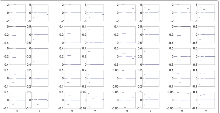
Figure 1 shows the estimated canonical loadings of all four SCCA methods in a typical run. As we can see, L1-SCCA cannot accurately recover the true signals. For those coefficients with sign swapped, it fails to recognize them. The FL-SCCA slightly improves L1-SCCA’s perfor-mance but cannot identify those coefficients with sign changed either. Our GOSC-SCCA successfully groups those nonzero features together, and accurately recognizes the coefficients whose signs are changed. No matter what structures are within the dataset, GOSC-SCCA is able to estimate true signals which are very close to the ground truth. Although KG-SCCA also recognizes the coeffi-cients with sign swapped, it is unable to recover every group of nonzero coefficients. For example, KG-SCCA misses two groups of nonzero features in terms ofvfor the second dataset. The results on synthetic datasets reveal that GOSC-SCCA can not only estimate stronger corre-lation coefficients than the competing methods, but also identifies more accurate and cleaner canonical loadings.
Evaluation on real neuroimaging genetics data
Data used in the preparation of this article were obtained from the Alzheimer’s Disease Neuroimaging Initiative (ADNI) database (adni.loni.usc.edu). The ADNI was launched in 2003 as a public-private partnership, led by Principal Investigator Michael W. Weiner, MD. The primary goal of ADNI has been to test whether serial
The A uthor(s) BMC Systems B iology 2016, 10 (Suppl 3):68 Page 341 of 380
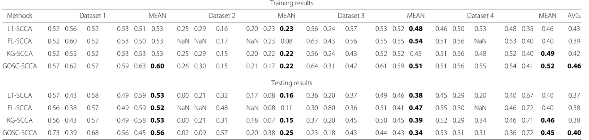
Table 15-fold cross-validation results on synthetic data
Training results
Methods Dataset 1 MEAN Dataset 2 MEAN Dataset 3 MEAN Dataset 4 MEAN AVG.
L1-SCCA 0.52 0.56 0.52 0.53 0.51 0.53 0.25 0.29 0.16 0.20 0.23 0.23 0.56 0.24 0.57 0.53 0.52 0.48 0.46 0.50 0.53 0.48 0.35 0.46 0.43
FL-SCCA 0.52 0.60 0.52 0.53 0.50 0.53 NaN NaN 0.17 NaN 0.23 0.08 0.63 0.43 0.56 0.55 0.55 0.54 0.51 0.56 NaN 0.53 0.40 0.40 0.39
KG-SCCA 0.52 0.55 0.52 0.53 0.53 0.53 0.25 0.29 0.15 0.20 0.22 0.22 0.56 0.24 0.43 0.52 0.52 0.45 0.51 0.56 0.48 0.52 0.40 0.49 0.42 GOSC-SCCA 0.57 0.62 0.57 0.59 0.63 0.60 0.26 0.30 0.15 0.21 0.17 0.22 0.64 0.31 0.42 0.61 0.59 0.51 0.51 0.56 0.55 0.54 0.41 0.52 0.46
Testing results
L1-SCCA 0.57 0.43 0.58 0.49 0.59 0.53 0.00 0.21 0.32 0.17 0.08 0.16 0.36 0.20 0.37 0.49 0.46 0.38 0.45 0.29 0.20 0.40 0.67 0.40 0.37
FL-SCCA 0.56 0.38 0.57 0.49 0.59 0.52 NaN NaN 0.48 NaN 0.08 0.11 0.30 0.80 0.36 0.51 0.41 0.47 0.55 0.30 NaN 0.46 0.72 0.40 0.38
KG-SCCA 0.56 0.43 0.57 0.49 0.58 0.53 0.00 0.21 0.31 0.18 0.07 0.15 0.37 0.20 0.45 0.50 0.45 0.39 0.52 0.29 0.34 0.46 0.71 0.46 0.38 GOSC-SCCA 0.73 0.39 0.68 0.56 0.45 0.56 0.02 0.09 0.57 0.20 0.38 0.25 0.23 0.18 0.43 0.44 0.43 0.34 0.53 0.31 0.31 0.36 0.72 0.45 0.40 The estimated correlation coefficients and their MEAN are shown. ’NaN’ means a method fails to estimate a pair of canonical loadings. ’0.00’ means a very small correlation coefficients. ’AVG.’ denotes the MEAN across all four datasets. The best values and those that are NOT significantly worse than the best ones (t-test withp-value smaller than 0.05) are shown in bold
Fig. 1Canonical loadings estimated on four synthetic datasets. The first column is for Dataset 1, and the second column is for Dataset 2, and so forth. For each dataset, the weights ofuare shown on the left panel, and those ofvare on the right. The first row is the ground truth, and each remaining row corresponds to a specific method: (1) Ground Truth. (2) L1-SCCA. (3) FL-SCCA. (4) KG-SCCA. (5) GOSC-SCCA
magnetic resonance imaging (MRI), positron emission tomography (PET), other biological markers, and clini-cal and neuropsychologiclini-cal assessment can be combined to measure the progression of mild cognitive impairment (MCI) and early Alzheimer’s disease (AD). For up-to-date information, see www.adni-info.org.
Table 2 contains the characteristics of the ADNI dataset used in this work. Participants including 568 non-Hispanic Caucasian subjects, including 196 healthy control (HC), 343 MCI and 28 AD participants. How-ever, many participants’s data are incomplete due to various factors such as data loss. After cleaning those participants with incomplete information, we get 282 par-ticipants in our experiments. The genotype data were downloaded from LONI (adni.loni.usc.edu), and the pre-processed [11C] Florbetapir PET scans (i.e., amyloid imaging data) were also obtained from LONI. Before con-ducting the experiment, the amyloid imaging data had been preprocessed and the specific pipeline could be found in [14]. These imaging measures were adjusted by Table 2Real data characteristics
HC MCI AD Num 196 343 28 Gender(M/F) 102/94 203/140 18/10 Handedness(R/L) 178/18 309/34 23/5 Age (mean±std.) 74.77±5.39 71.92±7.47 75.23±10.66 Education (mean±std.) 15.61±2.74 15.99±2.75 15.61±2.74
removing the effects of the baseline age, gender, educa-tion, and handedness via the regression weights derived from HC participants. We finally obtained 191 region-of-interest (ROI) level amyloid measurements which were extracted from the MarsBaR AAL atlas. We included four genetic markers, i.e., rs429358, rs439401, rs445925 and
rs584007, from the known AD risk geneAPOE. We intend
to investigate if our GOSC-SCCA could identify this widely known associations between amyloid deposition
andAPOESNPs.
Shown in Table 3 are the 5-fold cross-validation results of various SCCA methods. We observe that GOSC-SCCA and KG-SCCA obtain similar correlation coefficients on every run, including the training performance and testing performance. Besides, they both are significantly better than L1-SCCA and FL-SCCA, which is consistent with the analysis in [14]. This result shows that GOSC-SCCA can improve the ability of identifying interesting imag-ing genetic associations compared with L1-SCCA and FL-SCCA.
Figure 2 contains the estimated canonical loadings obtained from 5-fold cross-validation. To facilitate the interpretation, we employ the heat map for this real
data. Each row denotes a method, and u(genetic
mark-ers) is shown on the left panel and v (imaging
mark-ers) is on the right. As we can see, on the genetic side, all four SCCA exhibit similar canonical loading pattern. Since every SCCA here incorporates the lasso (1-norm),
The Author(s)BMC Systems Biology2016,10(Suppl 3):68 Page 343 of 380
Table 35-fold cross-validation results on real data
Methods Training results MEAN Testing results MEAN
L1-SCCA 0.50 0.50 0.53 0.53 0.54 0.52 0.56 0.61 0.45 0.47 0.38 0.49
FL-SCCA 0.44 0.43 0.46 0.45 0.46 0.45 0.49 0.56 0.39 0.43 0.37 0.45
KG-SCCA 0.53 0.52 0.55 0.54 0.56 0.54 0.56 0.61 0.47 0.52 0.45 0.52
GOSC-SCCA 0.53 0.52 0.55 0.55 0.56 0.54 0.56 0.62 0.47 0.51 0.45 0.52
The estimated correlation coefficients and their MEAN are shown. The best correlation coefficients and those that are NOT significantly worse than the best ones (t-test with p-value smaller than 0.05) are shown in bold
is a widely known AD risk marker, with those irrele-vant ones discarded to assure sparsity. On the imaging side, L1-SCCA identifies many signals which is hard to interpret. FL-SCCA fuses those adjacent features together due to its pairwise smoothness, which can be easily observed from the figure. But it is difficult to interpret either. GOSC-SCCA and KG-SCCA perform similarly again in this run. They both identify the imaging sig-nals in accordance with the findings in [20]. It is easily to observe that they estimated a very clean signal pat-tern, and thus is easy to conduct further investigation. Recall the results in Table 3, the association between the marker rs429358 and the amyloid accumulation in the brain is relatively strong, and thus the signal can be well captured by both KG-SCCA and GOSC-SCCA. In addi-tion, the correlations among the imaging variables and those among genetic variables are high enough so that the signs of these correlations can hardly be impeded by the noises. That is, the signs of sample correlations tend to be correctly estimated. Therefore, KG-SCCA does not suffer sign directionality issue, and so performs similarly
to GOSC-SCCA. However, if some sample correlations are not very strong and their signs are mis-estimated, KG-SCCA may not work very well (see the results of the second synthetic dataset). In summary, this reveals that our method has better generalization ability, and could identify biologically meaningful imaging genetic associations.
Discussion
In this paper, we have proposed a structured SCCA method GOSC-SCCA, which intended to reduce the esti-mation bias caused by the incorrect sign of sample cor-relation. GOSC-SCCA employed the GOSCAR (Graph OSCAR) regularizer which is an extension of the popu-lar penalty OSCAR. The GOSC-SCCA could pull those highly correlated features together no matter that they were positively correlated or negatively correlated. We also provide a theoretical quantitative description of the grouping effect of our SCCA method. An effective algo-rithm was also proposed to solve the GOSC-SCCA prob-lem and the algorithm was guaranteed to converge. 1 2 3 4 5 L1-SCCA 1 2 3 4 5 FL-SCCA 1 2 3 4 5 KG-SCCA -0.25 -0.2 -0.15 -0.1 -0.05 0 0.05 0.1 0.15 0.2 0.25 1 2 3 4 5 rs429358 GOSC-SCCA -0.25 -0.2 -0.15 -0.1 -0.05 0 0.05 0.1 0.15 0.2 0.25 Frontal
Fig. 2Canonical loadings estimated on the real dataset. Each row corresponds to a SCCA method: (1) L1-SCCA. (2) FL-SCCA. (3) KG-SCCA. (4) GOSC-SCCA. For each row, the estimated weights ofuare shown on the left figure, and those ofvon the right
We evaluated GOSC-SCCA and three other popular SCCA methods on both synthetic datasets and a real imaging genetics dataset. The synthetic datasets con-sisted of different ground truth, i.e. different correlation coefficients and canonical loadings. GOSC-SCCA was capable of consistently identifying strong correlation coefficients on both training set and testing set, and either outperformed or performed similarly to the com-peting methods. Besides, GOSC-SCCA successfully and accurately recognized the signals which were the closest to the ground truth when compared with the competing methods.
The results on the real data showed that both GOSC-SCCA and KG-GOSC-SCCA could find an important association
between the APOE SNPs and the amyloid burden
mea-sure in the frontal region of the brain. KG-SCCA performs similarly to GOSC-SCCA on this real data largely because of the strong correlations between the variables within the genetic data, as well as those within the imaging data. In this case, the signs of the correlation coefficients between these variables tend to be correctly calculated, and so KG-SCCA does not have the sign directionality issue. On the other hand, if the correlations among some variables are not very strong, the performance of KG-SCCA can be affected by the mis-estimation of some correlation signs. In this case, GOSC-SCCA, which is designed to overcome the sign directionality issue, is expected to perform better than KG-SCCA. This fact has already been validated by the results of the second synthetic dataset.
The satisfactory performance of GOSC-SCCA, coupled with its theoretical convergence and grouping effect, demonstrates the promise of our method as an effective structured SCCA method in identifying meaningful bi-multivariate imaging genetic associations. The following are a few possible future directions. (1) Note that the
iden-tified pattern between theAPOE genotype and amyloid
deposition is a well-known and relatively strong imaging genetic association. Thus one direction is to apply GOSC-SCCA to more complex imaging genetic data for revealing novel but less obvious associations. (2) The data tested in this study is brain wide but targeted only atAPOESNPs. Another direction is to apply GOSC-SCCA to imaging genetic data with higher dimensionality, where more effective and efficient strategies for parameter tuning and cross-validation warrant further investigation. (3) The third direction is to employ GOSC-SCCA as a knowledge-driven approach, where pathways, networks or other relevant biological knowledge can be incorporated in the model to aid association discovery. In this case, comparative study can also been done between GOSC-SCCA and other state-of-the-arts knowledge-guided SCCA methods in bi-multivariate imaging genetics analyses.
Conclusions
We have presented a new structured sparse canonical analysis (SCCA) model for analyzing brain imaging genet-ics data and identifying interesting imaging genetic asso-ciations. This SCCA model employs a regularization item based on the graph octagonal selection and clustering algorithm for regression (GOSCAR). The goal is twofold: (1) encourage highly correlated features to have similar canonical weights, and (2) reduce the estimation bias via removing the requirement of pre-defining the sign of the sample correlation. As a result, it could pull highly corre-lated features together no matter whether they are posi-tively or negaposi-tively correlated. Empirical results on both synthetic and real data have demonstrated the promise of the proposed method.
Acknowledgements
At Indiana University, this work was supported by NIH R01 LM011360, U01 AG024904, RC2 AG036535, R01 AG19771, P30 AG10133, UL1 TR001108, R01 AG 042437, R01 AG046171, and R03 AG050856; NSF IIS-1117335; DOD W81XWH-14-2-0151, W81XWH-13-1-0259, and W81XWH-12-2-0012; NCAA 14132004; and CTSI SPARC Program. At University of Texas at Arlington, this work was supported by NSF CCF-0830780, CCF-0917274, DMS-0915228, and IIS-1117965. At University of Pennsylvania, the work was supported by NIH R01 LM011360, R01 LM009012, and R01 LM010098.
Data collection and sharing for this project was funded by the Alzheimer’s Disease Neu-roimaging Initiative (ADNI) (National Institutes of Health Grant U01 AG024904) and DOD ADNI (Department of Defense award number W81XWH-12-2-0012). ADNI is funded by the National Institute on Aging, the National Institute of Biomedical Imaging and Bioengi-neering, and through generous contributions from the following: AbbVie, Alzheimer’s Asso-ciation; Alzheimer’s Drug Discovery Foundation; Araclon Biotech; BioClinica, Inc.; Bio-gen; Bristol-Myers Squibb Company; CereSpir, Inc.; Eisai Inc.; Elan Pharmaceuticals, Inc.; Eli Lilly and Company; EuroImmun; F. Hoffmann-La Roche Ltd and its affiliated company Genentech, Inc.; Fujirebio; GE Healthcare; IXICO Ltd.; Janssen Alzheimer Immunotherapy Research & Development, LLC.; Johnson & Johnson Pharmaceutical Research & Develop-ment LLC.; Lumosity; Lundbeck; Merck & Co., Inc.; Meso Scale Diagnostics, LLC.; Neu-roRx Research; Neurotrack Technologies; Novartis Pharmaceuticals Corporation; Pfizer Inc.; Piramal Imaging; Servier; Takeda Pharmaceutical Company; and Transition Therapeu-tics. The Canadian Institutes of Health Research is providing funds to support ADNI clinical sites in Canada. Private sector contributions are facilitated by the Foundation for the Na-tional Institutes of Health (www.fnih. org). The grantee organization is the Northern Califor-nia Institute for Research and Education, and the study is coordinated by the Alzheimer’s Disease Cooperative Study at the University of California, San Diego. ADNI data are dis-seminated by the Laboratory for Neuro Imaging at the University of Southern California.
Declarations
Publication charges for this article have been funded by the corresponding author.
This article has been published as part ofBMC Systems BiologyVolume 10 Supplement 3, 2016: Selected articles from the International Conference on Intelligent Biology and Medicine (ICIBM) 2015: systems biology. The full contents of the supplement are available online at
http://bmcsystbiol.biomedcentral.com/articles/supplements/volume-10-supplement-3.
Availability of data and materials
Data used in the preparation of this article were obtained from the Alzheimer’s Disease Neuroimaging Initiative (ADNI) database (adni.loni.usc.edu).
Authors contributions
LD, JM, AS, and LS: overall design. LD, HH, and MI: modeling and algorithm design. LD and JY: experiments. SK, SR, and AS: data preparation and result evaluation. LD, JY and LS: manuscript writing. All authors read and approved the final manuscript.
The Author(s)BMC Systems Biology2016,10(Suppl 3):68 Page 345 of 380
Competing interests
The authors declare that they have no competing interests.
Consent for publication
Not applicable.
Ethics approval and consent to participate
Not applicable.
Author details
1School of Medicine, Indiana University, Indianapolis, USA.2Computer Science
& Engineering, University of Texas at Arlington, Arlington, USA.3Rose-Hulman
Institute of Technology, Terre Haute, USA.4School of Medicine, University of Pennsylvania, Philadelphia, USA.
Published: 26 August 2016
References
1. Vounou M, Nichols TE, Montana G. Discovering genetic associations with high-dimensional neuroimaging phenotypes: A sparse reduced-rank regression approach. NeuroImage. 2010;53(3):1147–59.
2. Parkhomenko E, Tritchler D, Beyene J. Sparse canonical correlation analysis with application to genomic data integration. Stat Appl Genet Mol Biol. 2009;8(1):1–34.
3. Witten DM, Tibshirani R, Hastie T. A penalized matrix decomposition, with applications to sparse principal components and canonical correlation analysis. Biostatistics. 2009;10(3):515–34.
4. Chen X, Liu H, Carbonell JG. Structured sparse canonical correlation analysis. In: International Conference on Artificial Intelligence and Statistics, JMLR Proceedings 22, JMLR.org; 2012.
5. Chen X, Liu H. An efficient optimization algorithm for structured sparse cca, with applications to eqtl mapping. Stat Biosci. 2012;4(1):3–26. 6. Chi EC, Allen G, Zhou H, Kohannim O, Lange K, Thompson PM, et al.
Imaging genetics via sparse canonical correlation analysis. In: Biomedical Imaging (ISBI), 2013 IEEE 10th Int Sym On; 2013. p. 740–3.
doi:10.1109/ISBI.2013.6556581.
7. Lin D, Calhoun VD, Wang YP. Correspondence between fMRI and SNP data by group sparse canonical correlation analysis. Medical image analysis. 2014;18(6):891–902.
8. Du L, Yan J, Kim S, Risacher SL, Huang H, Inlow M, Moore JH, Saykin AJ, Shen L. A novel structure-aware sparse learning algorithm for brain imaging genetics. In: International Conference on Medical Image Computing and Computer Assisted Intervention. Berlin, Germany: Springer; 2014. p. 329–36.
9. Witten DM, Tibshirani RJ. Extensions of sparse canonical correlation analysis with applications to genomic data. Stat Appl Genet Mol Biol. 2009;8(1):1–27.
10. Chen J, Bushman FD, et al. Structure-constrained sparse canonical correlation analysis with an application to microbiome data analysis. Biostatistics. 2013;14(2):244–58.
11. Bondell HD, Reich BJ. Simultaneous regression shrinkage, variable selection, and supervised clustering of predictors with oscar. Biometrics. 2008;64(1):115–23.
12. Li C, Li H. Network-constrained regularization and variable selection for analysis of genomic data. Bioinformatics. 2008;24(9):1175–82. 13. Yang S, Yuan L, Lai YC, Shen X, Wonka P, Ye J. Feature grouping and
selection over an undirected graph. In: Proceedings of the 18th ACM SIGKDD International Conference on Knowledge Discovery and Data Mining. New York, USA: ACM; 2012. p. 922–30.
14. Yan J, Du L, Kim S, Risacher SL, Huang H, Moore JH, Saykin AJ, Shen L. Transcriptome-guided amyloid imaging genetic analysis via a novel structured sparse learning algorithm. Bioinformatics. 2014;30(17):564–71. 15. Hardoon D, Szedmak S, Shawe-Taylor J. Canonical correlation analysis:
An overview with application to learning methods. Neural Comput. 2004;16(12):2639–64.
16. Nie F, Huang H, Cai X, Ding CH. Efficient and robust feature selection via joint 2, 1-norms minimization. In: Advances in Neural Information Processing Systems. Massachusetts, USA: The MIT Press; 2010. p. 1813–21. 17. Grosenick L, Klingenberg B, Katovich K, Knutson B, Taylor JE.
Interpretable whole-brain prediction analysis with graphnet. NeuroImage. 2013;72:304–21.
18. Zou H, Hastie T. Regularization and variable selection via the elastic net. J Royal Stat Soc Ser B (Stat Method). 2005;67(2):301–20.
19. Lorbert A, Eis D, Kostina V, Blei DM, Ramadge PJ. Exploiting covariate similarity in sparse regression via the pairwise elastic net. In: International Conference on Artificial Intelligence and Statistics, JMLR Proceedings 9, JMLR.org; 2010. p. 477–84.
20. Ramanan VK, Risacher SL, Nho K, Kim S, Swaminathan S, Shen L, Foroud TM, Hakonarson H, Huentelman MJ, Aisen PS, et al. Apoe and bche as modulators of cerebral amyloid deposition: a florbetapir pet genome-wide association study. Mole psychiatry. 2014;19(3):351–7.
• We accept pre-submission inquiries
• Our selector tool helps you to find the most relevant journal • We provide round the clock customer support
• Convenient online submission • Thorough peer review
• Inclusion in PubMed and all major indexing services • Maximum visibility for your research
Submit your manuscript at www.biomedcentral.com/submit