Optimizing Logistic Regression Coefficients for Discrimination and Calibration Using Estimation of Distribution Algorithms.

Optimizing logistic regression coefficients

for discrimination and calibration using

estimation of distribution algorithms

V. Kobles • C. Bielza • P. Larranaga • S. Gonzalez -L. Ohno-Machado

Abstract Logistic regression is a simple and efficient supervised learning algorithm for estimating the probability of an outcome or class variable. In spite of its simplicity, logistic regression has shown very good performance in a range of fields. It is widely accepted in a range of fields because its results arc easy to interpret. Fitting the logistic regression model usually involves using the principle of maximum likelihood. The Newton-Raphson algorithm is the most common numerical approach for obtaining the coefficients maximizing the likelihood of the data.

This work presents a novel approach for fitting the logistic regression model based on estimation of distribution algorithms (EDAs), a tool for evolutionary computation. EDAs are suitable not only for maximizing the likelihood, but also for maximizing the area under the receiver operating characteristic curve (AUC).

Thus, wc tackle the logistic regression problem from a double perspective: likelihood-based lo calibrate the model and AUC-bascd to discriminate between the different classes, Under tliese two objectives of calibration and discrimination, the Pareto front can he obtained in our EDA framework. These fronts are compared with Ihosc yielded by a multiobjcclivc EDA recently introduced in the literature.

Keywords Logistic regression • Evolutionary algorithms • Estimation of distribution algorithms • Calibration and discrimination

1 Introduction

Logistic regression modeling is employed in many fields (Hosmer and Lemeshow

2000). The outcome variable is binary, while the explanatory variables are of any type, lending great, flexibility l.o this approach. Expcrimenial results have shown that logistic regression can perform at least as well as a more complex classifier in a vari-ety of data sets (liaumgartner et al. 2004; Kiang 2003), and this approach compared favorably with many supervised machine learning techniques: k-nearest neighbors, discriminant analysis, neural networks, support vector machines, and decision trees.

As in other simpler regression models, logistic regression applies the maximum likelihood principle for parameter estimation. Tire model that linearly relates the log of the odds of the response and the explanatory variables gives rise to complex nonlin-ear likelihood equations in the unknown parameters (Ryan 1997). Therefore, special numerical methods for their solution are required.

The so-called Newton-Raphson method is commonly used to solve the likelihood equations numerically. Although the method requires inverting a matrix and exhibits some dependence on the initial starting conditions for convergence to be guaranteed, it shows good performance overall (Minka 2003), One of the aims of the current paper is to tackle this maximization problem for parameter estimation by using a recent op-timization heuristic called estimation of distribution algorithms (LiDAs) (Larrafiaga and Lozano 2002). In this sense, we contribute towards tire (currently poor) applica-tion of optimizaapplica-tion heuristics in statistic estimaapplica-tion and modelling problems (Winker and Oilli 2004).

LDAs are evolutionary algorithms that are among the best-known stochastic population-based search methods. These algorithms construct an explicit probabil-ity model from a set of selected solutions which is then conveniently used to gener-ate new promising solutions in the next iteration of the evolutionary process. Other evolutionary algorithms, like genetic algorithms, have been used in logistic regres-sion but for performing feature subset selection (Vinterbo and Ohno-Machado 1999a;

Nakamichi et al. 2004), not for estimating the parameters or investigating the model performance from several points of view. To our knowledge, this is the first explo-ration on how EDAs can be used in this context.

The search for the parameters, both in a numerical or in an evolutionary way, tries to attain an appropriate model in the sense of maximizing the chances of obtaining Ihc data given Ihc filled model. The proximity of the true and the observed probabil-ity for a given set of observations, usually measured using calibration indices, is an important criterion of a model performance, However, it does not suffice. The logistic regression model outputs Ihc probability of a certain event occurring. This probabil-ity can be used to predict the class. For classification, high discriminatory abilprobabil-ity to differentiate between the classes is at least as important as calibration. In fact, the recommendation of assessing the model performance by considering both calibra-tion and discriminacalibra-tion has been clearly asserted, e.g., in seminal texts on logistic regression (see Hosmer and Lemeshow 2000, p. 163).

Since good calibration does not necessarily mean good discrimination and vice versa, both types of measures should be analyzed in logistic regression models. Therefore, we specifically study the behavior of two model performance measures:

the maximum (log) likelihood (for calibration) and the area under the receiver oper-ating characteristic curve (AUC) (for discrimination).

Among the most outstanding strengths, our new EDA framework can be flexible enough to cope with the parameter estimation when the optimization is based on cal-ibration or on discrimination, or even on other model performance measures like the Brier score or any multi-objective measure. Moreover, the bi-objcclivc space of cali-bration against discrimination can be explored to depict the relationship between both objectives, allowing us to estimate the Pareto front with the non-dominated points.

The paper is organized as follows. Section 2 reviews the logistic regression model and the derivation of the likelihood equations. Section 3 includes the model perfor-mance measures we will use to assess calibration and discrimination. Section 4 deals with different estimation methods of performance when the model faces future (un-seen) data. Section 5 describes a method for searching the logistic regression para-meters based on EDAs, emphasizing the advantages of this new approach. Section 6

shows the experiments with severai data sets and the potentiality of our method. Sec-tion 7 highlights the benefits of our new approach, finally, we discuss in Sect. 8 the conclusions and lines of future research.

2 Logistic regression

Logistic regression (Hosmer and Lemeshow 2000) is a standard method to describe the relationship between a response (or dependent) variable which is binary and sev-eral explanatory (or predictor) variables called covariates. When it is used for clas-sification purposes, the response variable is the class variable C predicted through covariates X\ Xj.. In this context, logistic regression becomes a powerful super-vised classification paradigm lhat provides explicit probabilities of classification that can be used to provide class label information. This approach falls into the category of discriminative classifiers, in the sense that they model the probability of the class given tiie covariates, in contrast to generative eiassifiers that model the joint probabil-ity of the ciass and the covariates (Ng and Jordan 2001). As opposed to other methods like discriminant analysis, strong assumptions like normal dislribulion of the covari-ates given the class arc not required. Also, covaricovari-ates can be given in a quantitative (continuous or discrete) or qualitative scale.

The logistic regression classifier is induced from a (training) data set I V contain-ing N independent samples Z?# = {(cy, Xji,,.,,jcy*), j — 1 , . . . , N}, drawn from the joint probability distribution on (C, X\,..., X*). In this paper, we focus on the two category ciassification problem, aithough the ideas could be readily extended to the multi-category case. Thus, C can only take 0 and 1 values, where label cj = 1 means lhat Ihc ylh input pattern x;- = (JC^J, .. .,Xjk) is in the first class (i.e., observation j has the feature that C represents), while Cj — 0 means xy does not have the feature, and therefore belongs to the other class. The classification model will be used for assigning labels cy to new instances that are not part of the training set, and therefore are only characterized with the values of the predictor variables.

Let % denote P(C = l|x) = P(C = 1\X\ = xx Xk = **). Then the fc#ft modei is defined as:

l o g - ^ - = A> + jSiXi+ . . - + & ) » , (1) or equivalentiy,

(2)

where ^ = (fto, ft ft) denotes the vector of regression coefficients including a constant or intercept

ft-Therefore, the model specifics nx as the dependent variable to be a function of the predictor variables. Since C is dich.Otom.OUS, its expected value is E(C\x) — TTX, and we search for a relationship between the expected response and the covariates.

Regression coefficients arc usually estimated from the data by means of the max-imum likelihood estimation method. Given the training data set, the likelihood func-tion is £(/?) = riy=] ^xj (1 — Xxj)1~Ci, where xXj is stated in (2). Maximum like-lihood estimators (MLR) ft are obtained by maximizing C with respect to /?, or equivalentiy, by maximizing log/", with respect to ft

We have that

N

log£03) = J2(cjloe^x,- + 0 -Cj)log(l -7tXj))

N N

= J2

J

'°g

r^ir

+

£

l0

-

(

l

- **

}

and using (1) and (2),

N N

log£(0) = J2

J (#> + ft*Ji + ' ' ' + &*/*) - E

§(l + e ^ + ^ '

-

^ > ) .

Thus, the following system of k +1 equations and k + 1 parameters—called the likelihood equations—has to be solved:

aiog£(/?) £ £

«"+-+***3

= X)*/*/* - ][^x/t r

<¥* £-,*>* ^ ** I + e0O+"<+fts9»)

= 0.

Unfortunately, there is no analytical solution of these nonlinear equations for ft, but we may resort to using numerical optimization metliods. Among tliese, a general

choice is the Newton-Raphson numerical procedure (TTiisted 1988) in which each iteration provides an updating formula given by

r

= r

+(x

wxr

x

<€-£},

where # = (#>, fiu • • • * Pk\ c denotes the vector of response values CJ (j =

1,...,N), X denotes an N x (k + 1) matrix with each row given by (l,xy), K denotes the vector of estimated values at that iteration, i.e., its j'lh-coniponeni. is JTXJ. = [1 + e~$> +Prx&+-+Pk ^ l- 1, j = 1 , . . .. N, and W denotes a

diago-nal matrix with elements ^ - ( l — ^x,-}. This formula is used until a convergence criterion is achieved. Common convergence criteria consist of the detection of neg-ligible changes in the log likelihood function, in the parameter estimates, or in the predictions. No single criterion appears superior to the others. In regard to starting estimates, the ones obtained using discriminant analysis turn out to be good and may speed up the convergence (Ryan 1997).

Minka (2003) compares eight different numerical algorithms for computing l.hc MLEs in terms of computational complexity (total floating-point operations) and per-formance (log likelihood value achieved), The Newton-Raphson algorithm shows excellent performance and a rapid convergence rate.

Therefore, it may seem hard to design a better algorithm to approximate the fa MLEs (or logistic regression. Since our estimation problem is an optimization prob-lem, a promising alternative would be to try some optimization heuristics, which sur-prisingly have not been very commonly used in statistical estimation and modelling problems (Winker and Gilli 2004). We introduce here the estimation of distribution algorithms (EDAs) that, to the best of our knowledge, have never been used in this context. As far as evolutionary algorithms are concerned, we only know of a genetic algorithm employed to select variables in logistic regression (Vinterbo and Ohno-Machado 1999a; Nakamichi el. al. 2004), not in the estimation problem.

The log£ function guides the search of fa's, trying to produce a model that fits, i.e., the observed sample values of the response variable agree with the values pre-dicted by the model (or fitted values). This goodness-of-fit informs us about the ef-fectiveness of the model in describing the response variable. A good fit provides a calibrated model.

However, when classification is a goal of the modeling and estimated probabilities are used to predict the class membership, the discrimination between the different classes may not be accurate even if the model fits the data well. Situations in which file logistic regression fits the data properly but yields poor classification have been rcporlcd elsewhere (sec Hosmcr and Ecmcshow 2000, p. 156 and p. 163).

Therefore, both calibration and discrimination measures should be analyzed in logistic regression models, Among other interesting findings, we show that EDAs are flexible enough to cope with the estimation of jS's when the optimization is based on any of those measures.

3 A l t ' as a model performance measure in logistic regression

As noted above, good calibration does not necessarily entail good discrimination and vice versa. A seminal text on logistic regression claims that "model performance

should be assessed by considering both calibration and discrimination" (see Ilosmer and T.emeshow 2000, p. 163) and this is also our viewpoint.

One solution taken in the literature is to start off with a model that has good dis-crimination and then adjust its calibration, what is called model recalibmtion Harrell et al. (1984). In logistic regression, Harrell et al. (1996) propose shrinkage to re-calibrate. However, this increases calibration only when the testing set is relatively large (Steyerberg et al. 2004), which is not always the case in practice. Vinterbo and Ohno-Machado (1999b) propose to alter the estimated probabilities by applying a discrimination-preserving transformation, which is empirically determined from a linear regression on the points in the calibration plot to move them closer to the iden-tity line (the ideal calibration). A second transformation is still needed to keep the resulting predictions within 0 and 1. This method suffers from a number of limita-tions: It is not useful when the model gives the same estimates for every input, when the calibration plot points are spread in an alternating pattern around die identity line, or when many estimates are close to either 0 or 1.

The approach taken in this paper is different, since we search for a model that directly provides good overall performance by optimizing with respect to different performance measures with an evolutionary algorithm.

When classifying instances, since probabilistic model outputs are continuous, we have to transform those outputs into binary outcomes providing the predicted class. For a given cutpoinl. or threshold t e |0, 11, we can decide that the predicted class of an instance j is Cj — 1 if its estimated probability TT; > / and it is £j = 0 oth-erwise. Each t results in a sensitivity and specificity pair, The plot of the values of

1-specificity (false positive rate) against sensitivity (true positive rate) over all pos-sible cutpoints is the receiver operating characteristic (ROC) curve (see e.g. Pepe

2003).

ROC curves describe the predictive behavior of a classifier independently of class distributions or error costs. Its use as a metric for comparing algorithms rather than using the classification error rate has been widely justified (see, e.g., Provost et al.

1998).

The ROC curve is commonly summarized by the area under the curve (AUC) (Hilden 1991; Bradley 1997). AUC ranges from 0 to 1, where perfect discrimination between both classes corresponds to an area of 1 (a horizontal line through the point (1,1)) and random classification corresponds to an area of 0.5 (the identity line).

There are many ways to compute the AUC (Eaweett 2003). We can use the trape-zoidal rule after connecting the ROC curve points by straight lines (Ilorton et al.

2004), which is a poor computational strategy, known to underestimate the AUC if Ihe number of points is limited (Hanlcy and McNeil 1982), AUC has an important statistical property: it is equivalent to the probability that the classifier will rank a randomly chosen positive instance higher than a randomly chosen negative in-stance. Thus, an intuitive way to proceed is by computing the concordance index or c-index, as follows. Let us create all the possible pairs of observations such that its first element has cj = 1 and the second element has CJ — 0. Then, the c-index is the proportion of the time that die observation with cj — 1 has the higher of the two probabilities, with tics resolved by tossing an unbiased coin (Harrell ct al. 1996;

the Mann—Whitney U statistic, which is another form of the Wilcoxon rank-sum test (Hajek el. al. 1999). Under limited information—like having only a single point of the ROC curve—approximations to the AUC can be computed (van den Hout 2003).

Other approximations, both parametric and non-parametric, have been proposed in Ihe large lil.erat.urc on the subject, see a review in Lasko el. al. (2005).

4 Model performance assessment

In the previous sections, we have introduced two performance measures of a model: log £ and AUC. To assess this performance that allows us to compare a model to other candidate models, its discrimination/calibration ability has to be checked on test data that is different from training data. By so doing, we estimate the generalization performance of our model.

Let us start our discussion by taking the error rate as the performance metric. After designing our logistic regression classifier, its (classification) error rate when using the model for classifying unseen (new) instances has to be estimated, or at least its expected error rale. A low error rate usually corresponds to high accuracy. When comparing error estimators, that should be as close as possible to the true error, one has to consider their bias and variance, since the composition of both defines the mean squared error. Unbiascdncss (or al. least a low degree of bias) and small variance are desirable. A large variance is of particular concern even with unbiasedness, since the estimate corresponding to a given sample can be often far from the actual error rate. Among these estimators, the resubstitulion estimator, where the error is directly computed on the sample data itself, is simply a very fast but usually optimistic (i.e., low-biased) cslimalor of the true error. Holdout error estimation, with a training set for the modeling and a test set for testing the classifier, requires large sample sizes.

However, cross-validation error estimation is the most widely used method and provides a nearly unbiased estimate of the future error rate although perhaps at the expense of some variance, hi k-fold cross-validation (Stone 1974), the data set is ran-domly partitioned into k folds of approximately equal size. Each time t e { 1 , 2 , . . . , k\ a fold is left out of the modeling process and used as a testing set. The cross-validation estimate of the error is computed by averaging the resulting error estimations from all folds. A 10-fold cross-validation will be the chosen method in this paper.

Any—more general—performance measures as log L and AUC may be estimated from the data in a way similar to the one used in estimating the error rate.

5 Estimating the logistic regression coefficients with estimation of distribution algorithms

As staled in Sect. 2, the likelihood equations to be solved in order to obtain the val-ues of parameters /So,..., jS^ cannot be resolved analytically (Hosmer and Lemeshow

2000). Several numerical algorithms for computing the MLE of the regression coef-ficients have been proposed in the literature (Minka 2003). However, the solutions provided by these procedures are likely to be improved in some circumstances.

In this section we present an introduction to estimation of distribution algorithms (EDAs), a recent population-based stochastic optimization heuristic (Larranaga and Lozano 2002). We also describe a method for searching the optimal values of the logistic regression coefficients based on EDAs in continuous domains.

5.1 Rsl.imat.ion of distribution algorithms

It is possible to use optimization heuristics as an alternative way for the estimation of regression parameters. These optimization heuristics can be divided into local and po-pulation-based search methods. Evolutionary algorithms are among the best-known stochastic population-based search methods. They start from a random population Of individuals—each of them representing a possible solution to the optimization problem—and iterate until some pre-defined stopping criterion is satisfied. At every iteration, usually called generation, a subset of individuals is selected. By applying some variation operators to the selected set, a new population is created. An exam-ple of evolutionary algorithms arc genetic algorithms (GAs) (Goldberg 1989). The distinguishing feature of GAs is the application of tlie recombination and mutation operators. As mentioned before, GAs have been used in combination with logistic re-gression only in the selection of the covariates to be included in the model (Vinterbo and Ohno-Machado 1999a; Nakamichi et al. 2004).

Another class of population-based search methods comprises those algorithms that use probabilistic modeling of the solutions instead of genetic operators. Estimation of distribution algorithms (Larrafiaga and Lozano 2002; Lozano et al. 2006) are evolu-tionary algorithms that construct an explicit probability model from a set of selected solutions. This model can capture, by means of probabilistic dependencies, relevant interactions among the variables of the problem. Tlie model can be conveniently used to generate new promising solutions.

Figure 1 shows a pseudo-code for a general EDA approach to optimization. At the beginning M individuals, each of them representing a point of the search space, are generated al random. These M individuals constitute the initial population and arc evaluated by means of a fitness function. In a first step of the algorithm, a number N (N < M) of individuals arc selected according to a selection method. Next, the

(i) D0 *- Generate M individuals randomly (ii) I = 1

(iii) do {

(iv) £>f£j <— Select N < M individuals from D/_i according to a selection method

(v) pi(z) — p{z\Dfti) ^— Estimate the joint probability distribution from the selected individuals

(vi) D[ 4- Sample M individuals (the new population) from pi(z) (vii) J until a stopping criterion is met.

induction of a multidimensional probabilistic model that reflects the interdependen-cies between the variables in these N individuals is carried out. The estimation of the joint density constitutes the bottleneck of EDAs, as different degrees of dependencies between the variables used to represent the individuals can be considered. In a third step, M new individuals-thc new population—are obtained from a simulation of the multidimensional probabilistic model learnt in the second step. These three steps are repeated until a stopping condition is met.

The main advantages of EDAs as compared to GAs arc: (i) they avoid designing ad hoc crossover and mutation operators, as well as the tuning of the values of several associated parameters; (ii) they are able to express in an explicit manner, by means of a joint probability distribution, the relationships between the different variables used to represent a point of the search space, and (iii) they can incorporate from the beginning some knowledge we can have about the problem by imposing conditional independence relationships between those variables. These advantages, as well as the difficulties of using real coded CAs, necessary in our problem, have led us to choose EDAs as better suited for this paper.

EDAs have been successfully applied in machine learning, for instance in learning Baycsian networks from data (Blanco el. al. 2003; Romero ct al. 2004), in feature subset selection (Inza et al. 2000), and in different optimization problems, within k-nearest neighbors, clustering and neural networks paradigms (Larranaga and Lozano

2002).

5.2 IJMDA^ approach for logistic regression

Let Z-:, with i = 0 , 1 , . . . ,k, represent a continuous random variable. A possible value Of Zj is denoted zi. Each continuous variable is associated with its corresponding parameter of the logistic regression model. In our case, z.i represents a value for pa-rameter fii. Similarly, we use Z = (Zo, Z\,..., Z#) to represent a k + 1 dimensional random variable and z — (zo, z\,..., z%.) to denote one of its possible values. In this sense, z — (zo, Zi, — Zk) refers to a value for the parameters jS = (/?o, Pi A ) -The joint density function over Z is denoted by p(z).

Tn order to reduce as much as possible the computational cost derived from the learning of the joint density function, p(z), we have chosen the EDA approach called UMDA^ (Larranaga et al. 2000). UMDAf9 assumes that at each generation ail

vari-ables arc independent and normally distributed. Tacking ihcse two assumptions into account, the joint density at each generation, pi(z), can be factorized as follows:

The 2(k + 1) parameters of the model, pu and an with J = 0 , 1 , . , . , k, have to be estimated at each generation by means of the sample mean and standard deviation calculated from the selected individuals.

We can use EDAs not only to obtain the values of the parameters $Q, fix,...(/fe

thai maximize the likelihood but also to optimize other model performance measures like the AUC, We propose the use of EDAs, specifically the UMDA'f approach, to build two new algorithms that use different fitness functions:

- UMDAjf-logL which goal is to obtain the /U's in a logistic regression model, with the highest log L value;

- UMDAf-AUC which goal is to obtain the /J's in a logistic regression model, with the highest AUC value.

Note that, unlike Ihc traditional procedures to find parameters /i,-'s as MLE, the EDA approach is able to use any optimization objective, regardless of its complexity or the lack of an explicit formula for its expression, like for tlie AUC objective.

The parameters used to run the proposed algorithms based on EDAs and the method used for assessing the convergence may vary depending on the specific prob-lem, The chosen values for our data sets are fully detailed in Sect, 6,2. As usual, the best individual in the last generation is chosen as solution.

Other EDA approaches that take into account more complex interactions among parameters $ ' s could be used, at the expense of the computational cost, but with the explicit modeling of their probabilistic conditional dependencies {see Larrafiaga and Lozano 2002, Chap. 2).

6 Experiments

6.1 Data sets

The experimental study was carried out with six different data sets, described as fol-lows:

- The B r e a s t cancer data set intends to distinguish benign tumors from malignant tumors (benign/malignant),

- The D i a b e t e s data set shows whether the patients have signs of diabetes (healthy/diabetes) according to World Health Organization criteria.

- The ICU data set contains patients who were pari, of a much larger study on sur-vival of patients following admission to an adult intensive care unit (ICU). The major goal of this study is to develop a logistic regression model (or another valid method) to predict the probability of in-hospital survival (died/lived).

- The P r o s t a t e cancer data set involves a study of patients with prostate cancer. The goat of the analysis is to determine if variables measured at a baseline exam can be used to predict whether the tumor has penetrated (penetrated/not penetrated) the prostatic capsule.

- The purpose of Ihc UIS data set is to compare treatment programs of different planned durations designed to reduce drug abuse and to prevent high-risk HIV behavior. The class variable is defined as having returned to drug use prior to the scheduled completion of the treatment program (remained drug free/ otherwise). - The goal of the A d u l t - r data set is to predict whether income exceeds $50

K/yr (> 50 K, < 50 K) based on census data. The original A d u l t data set in-cludes 48,842 instances. By randomly selecting 8,000 instances maintaining the same proportion of positive and negative cases, the corresponding reduced version A d u l t - r is the data set used here.

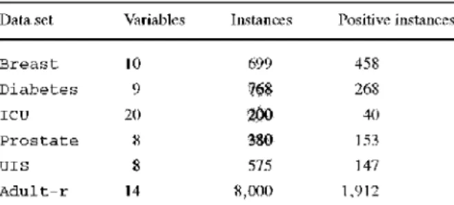
Table I I )ata sets

characteristics Data set

B r e a s t D i a b e t e s I C D P r o s t a t e D I S A d u l t - r Variables 10 9 20 8

s

The first, two and the last data sets come from the UCT machine learning repository (Newman et al. 1998). The remaining data sets were obtained from (Hosmer and Lemeshow 2000). Tahle 1 contains the number of variables, the number of instances and the number of positive instances (c; = 1) of each data set.

6.2 Implementation

To obtain the MLEs of /3's with the Newton-Raphson algorithm, we have used the R environment for statistical computing and graphics (R Development Core Team 2004;

Ihaka and Gentleman 1996), which is freely available, MLEs are computed using the g l m ( ) function that Lakes into account the change between successive steps in parameter estimates to assess the convergence of the algorithm. We have called this algorithm R-glm. Besides, we have used the s o m e r s 2 () R function included in the Hmisc package for estimating the AUC. This function computes tire e-index explained earlier.

For the new proposed algorithms based on EDAs, we have developed our own implementation in C++. EDAs were run with two different fitness goals: maximiz-ing log likelihood (UMDA^-logL) and maximizmaximiz-ing the area under the ROC curve (UMDAJ/-AUC).

The parameters used to run UMDAfG were (see Tig. 1): (i) population size of 200

individuals (M — 200), (ii) the best 100 individuals were selected for the learning step (JV = 100), and (iii) the change in the fitness value average between successive generations was chosen to assess the convergence of the algorithms. These parame-ters were tuned after some extra experiments.

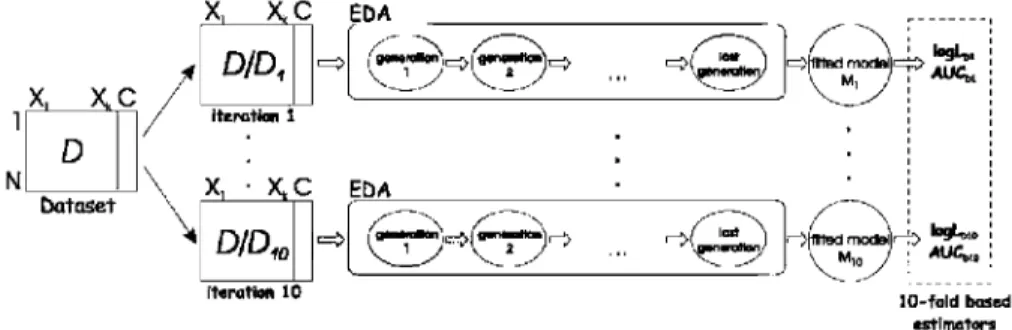
As commented in Sect. 4, a 10-fold cross-validation was used to estimate model performance measures, both in R-glm and UMDA';' algorithms (this process is shown in Fig. 2 for the EDA-based algorithms). Due to tlie stochastic nature of this validation method, each experiment was run five different times, therefore having a 5 x 10-fold cross-validation (Bouckaeit and Frank 2004).

6.3 Comparison of algorithms

Tabic 2 summarizes the experimental results reflecting the average and standard de-viation of the performance measures over all executions carried out widi R (R-glm) and the two EDA algorithms. Note that for each algorithm we show not only the optimized measure but also the other measure in order to get an insight into the rela-tionships between them.

1 N

x, xc

_{(~)^>(«T3^ ___ ^Q£)}

_'Th^y^n

Fig. 2 Assessing the performance of UMDAr algorithms using 10-fold cross-validation

Tabic 2 Summary of the experimental results reflecting the average and standard deviation of all perfor-mance measures over the five executions, besides the average computation time for each fold. A means that EDA exhibits a statistically significant better behavior when compared to R-glm (p-value < 0.05). V is for the opposite significance. Filled symbols are used for the performance measure that is being optimized by ihe associated algorithm

Daia sel Algorithm Model performance measures

\os£ AUC Compulation lime (s) B r e a s t D i a b e t e s ICU P r o s t a t e U I S A d u l t - r R-glm UMDA<?-logL UMDAj?-AUC R-glm U M D A ^ - l o g L U M D A p - A U C R-glm UMDAf-JogL H M D A ^ - A U C R-glm UMDA<?-logL IMD&f-AXJC R-glm U M D A ^ - l o g L U M D A p - A U C R-glm U M D A ^ - l o g l . U M D A ^ - A U C - 7 0 . 9 7 ± 2.34 - 7 0 . 3 6 ± 0.84 - 8 4 . 7 0 ± 6.20 V - 3 2 0 . 8 5 ± 1.60 - 3 1 9 . 4 8 ± 1.76 - 1 5 2 6 . 5 2 ± 241.56 V - 1 4 2 . 7 2 ± 2 5 . 7 0 - 1 3 8 . 6 7 ± 16.79 - 4 9 7 . 7 3 ± 4 0 . 1 9 V - 2 0 2 . 0 9 ± 2 . 1 8 - 1 9 9 . 2 5 ± 1.94 - 2 0 6 . 0 2 ± 2.60 V - 3 2 0 . 7 7 ± 0.64 - 3 1 8 . 9 8 ± 0 . 9 5 A - 4 8 5 . 1 5 ± 29.92 V - 2 8 3 2 . 4 8 ± 8.78 - 2 8 4 3 . 5 7 ± 5.37 - 1 2 8 2 1 . 5 3 ± 418.47 V 0.9936 ± 0.0003 0.9937 ± 0.0001 0.9930 ± 0 . 0 0 1 5 0.8298 ± 0.0008 0.8318 ± 0 . 0 0 1 1 0.8267 ± 0.0082 0.7754 ± 0.0183 0.7617 ± 0 . 0 0 6 8 0.7773 ± 0.0082 0.8017 ± 0 . 0 0 4 1 0.8066 ± 0 . 0 0 5 1 0.8096 ± 0.0076 i. 0.6220 ± 0.0030 0.6307 ± 0.0037 A 0.6417 ± 0.0106 A 0.8449 ± 0.0015 0.8442 ± 0.001 8 0.8447 ± 0.0012 0.24 2.80 3.13 0.32 4.24 5.48 0.49 4.66 9.89 0.20 1.82 2.84 0.18 3.99 6.94 1.59 218.37 371.59

The Mann-Whitney test was used to compute the statistical significance of the dif-ference between the algorithms. A A symbol (a V symbol) in a value means that the corresponding UDA algorithm reveals a statistically significant better (worse) behav-ior than R-gltn with a /rvalue < 0.05. Filled symbols arc used for the performance measure that is being optimized by the associated algorithm. The absence of the

sym-bol means that there was not enough evidence to reject the null hypothesis of equal behavior of the algorithms.

Several conclusions can be extracted from Table 2 with respect to the algorithms: - The UMDAG-logE algorithm achieves at least the same results as the R-glm

al-gorithm. Most of the Lime the differences arc negligible. In fact, there is only a statistically significant difference in the log£ value for the UIS data set in favor of the EDA (p — 0.01), see the second row of each data set, under the log £• col-umn. In contrast, R-glm is never statistically superior to the EDA. Note that in this case both algorithms are using the same fitness function, log£, but a completely different search strategy.

While optimizing log£, we can record the corresponding AUC (second row, last column). In this case, AUC as a complementary measure, exhibits the same behavior when the search is carried out using R-glm and EDA algoridims. There is one statistically significant difference in the AUC value for the UIS data set in favor of the EDA (/> = 0.007).

- The behavior of the UMDAG-AUC algorithm is now analyzed. Here we

com-pare the AUC outputted by UMDAG-AUC algorithm, which is its objective

func-tion, and the AUC corresponding with the model that R-glm finds (see the third row of each data set, under the AUC column). For B r e a s t , D i a b e t e s , ICU and A d u l t - r data sets, the differences are negligible. However, for P r o s t a t e (p — 0.05) and UIS (p — 0.007) data sets, EDA is again statistically superior to R-glm.

When we look at the log C values, recorded in our EDA algorithm as a comple-mentary measure not used for the optimization (third row of each data set, under the log C column), R-glm always displays statistically significant differences ver-sus EDA (p — 0.007 always except for die P r o s t a t e data set, with p = 0.03). Therefore, under (he same optimization problem of maximizing log£, our EDA (UMDAG-logL) algorithm behaves as a strong competitor of the R-glm algorithm,

achieving similar and sometimes better results.

On the contrary, when wc compare a certain measure yielded by algorithms that optimize different objectives, the results use to favor the algorithm that optimizes the measure. Thus, if we compare the log/", values outputted by the UMDAG-AUC

al-gorithm and the R-glm alal-gorithm, the latter alal-gorithm is better. However, when we

compare the AUC values outputted by the UMDAG-AUC algorithm and the R-glm

algorithm, both algorithms almost tie, with the EDA algorithm being slightly supe-rior.

Tn terms of computational time, EDA-bascd algorithms arc slower than R-glm, but required times are quite reasonable. For the first five data sets, while R-glm ranges between 0.18 s and 0.49 s, UMDAG-logL ranges between 1.82 s and 4.66 s mid

UMDAG-AUC ranges between 2,84 s and 9.89 s. For the A d u l t - r data set, with

more instances, R-glm needs 1.59 s while UMDAG-logE and UMDAG-AUC need

218.37 s and 371.59 s, respectively (see Table 2).

Note that optimizing an objective does not guarantee a good behavior of other pos-sible objectives. How calibration and discrimination measures arc related in logistic regression models is an aim in this paper and will be analyzed in die next subsections.

6.4 Joint evolution of performance measures

The results also show that optimizations with log£ as fitness function achieve good results in all performance measures while optimizations with AUG as fitness func-tion achieve only good results in AUG values. Just another point of view: optimizing calibration results in optimizing discrimination, but optimizing discrimination does not result in optimizing calibration. As discussal in Sect. 3, log£ is a calibration measure white AUC is a discrimination measure.

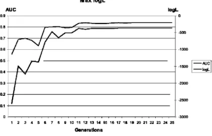
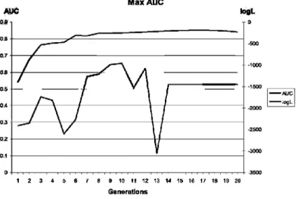
it is possible to verify this situation by analyzing the evolution of the performance measures during the optimizations of the different fitness functions. For the D i a -b e t e s data set, the evolution of each measure, AUC and log£, during the maxi-mization of tog L can be seen in Fig, 3, Similarly, the evolution during the maximiza-tion of AUC in the D i a b e t e s data set can be found in Fig. 4. The behavior on the other five data sets is analogous.

Note that each logistic regression model, that is, specific values for the parameters 00, fii,,.., pk, has associated AUC and log £ values represented in the curves of the figures, Since we have already compared the algorithms, from now on the models will be fitted by using the whole data set, i.e., by rcsubslitution.

As shown in Fig. 4 for the D i a b e t e s data set during AUC maximization, when AUG values become stable (generation 12) at approximately 0.839, log£ vaJues range from —3064 to -1073. However, as observed in Fig. 3, during log£ maxi-mization, when log/", values become stable (generation 18) at approximately -366, AUC also reaches good and stable values. This means that log £ optimization leads to AUC optimization but not vice versa.

Moreover, the final log£ values when maximizing AUC ait different depending on the execution. For example (see Table 2), in the D i a b e t e s data set with sta-ble final AUC values (mean 0.8267 with standard deviation 0.0082) there is a high

Max logL AUC logL -AUC -logL 1 2 3 4 5 B 7 S 9 10 11 II 13 14 15 18 17 1B 18 20 21 22 23 24 25 Generations

Max ADC

-AUC

HjgL

Fig. 4 Evolution of log £ and AUC in the UMDAf-AUC algorithm for the D i a b e t e s data set

Tabk'3 UMDA^-AUC algorithm final results of the five executions for D i a b e t e s Execution 1 2 3 4 5 Final log C -1440.478 -1413.735 -1395.572 -1096.662 -1407.625 Final AUC 0.8400 0.8397 0.8334 0.8398 0.8332

variance in the final log£ values (mean —1526.52 with standard deviation 241.56) because each of the executions reaches quite different search space points.

Table 3 reports the final log£ and AUC values of the logistic regression models that have been achieved in the five executions of the UMDA^-AUC algoritlim for the D i a b e t e s data set.

An explanation for this lies in the different shapes of the optimization functions. The log £ is a concave function of the /3 coefficient, and the free variation of /? in a convex set guarantees that tliere are no local maxima on the log-likelihood surface of a logistic regression model. That implies an easy-to-reach optimization, which also brings incidentally good values in other performance measures like AUC, as we have shown.

Nonetheless, die AUC surface has many local maxima, each one with similar AUC values but different log C values. This implies a harder optimization problem, with the added difficulty of having to be cautious with the (perhaps bad) log C value associated to a good AUC value obtained when maximizing the AUC function.

This is also observed in 1'ig. 5 that depicts the search space points that the liDA algorithms visited in the whole optimization process of the D i a b e t e s data set. For

o

3

..'••v:&&£CJ»

-•

•

•

-V,

J ^

Kig. 5 Performance measures, log£ vs. AUC, of all visited logistic regression models during the two EDA based optimization processes of the D i a b e t e s data set

each visited point the performance estimates of log £ and AUC arc plotted. The be-havior on the other five data sets is quite similar.

6.5 Pareto front in the calibration vs, discrimination space

Our previous experiments with EDAs have shown that optimizing log£ achieves good results in AUC. This provides the basis to develop an ad hoc method to explore promising regions of the bi-objcclivc space of calibration (log£) vs. discrimination (AUC). The method proceeds as follows. The EDA algorithm is run many times, each one with Hie same value of parameter fil() and different um (i = 0, 1,... ,k), both determining the normal density function of the UMDA£G model at the initialization

step, see Sect. 5.2. Parameter /^o is fixed as the component i of the solution achieved by IhcNcwlon-Raphson method. Parameter a,o is progressively increased to enlarge the space to be explored. Since log £ is the objective function for the EDA, this naive procedure leads to points with hopefully good values not only in log £, but in AUC.

In the bi-objective space, non-dominated points are of interest as optimal solutions in Ihc sense of not having any other point that is equal or better with respect to all the objective functions. The resulting set is the non-dominated or efficient set, also called Pareto front (Steuer 1986). Circles (magenta color) of Fig. 6 show the approximate Pareto front obtained by the ad hoc method described above.

Alternative ways to find the non-dominated points would consist of undertaking bi-objective optimizations. A recent research by Zhang cl al. (2008) proposes a reg-ularity model based multiobjective EDA (RM-MEDA) for continuous multiobjective optimization problems. Under mild smoothness conditions, it holds that the Pareto set is apiecewise continuous manifold of dimension r — 1, where r is die number of objectives. The idea is to exploit explicitly this regularity property of die Pareto set in building the probabilistic model the EDA needs. EDA constructs the probability

Breast -80 Log llkollhood 0,9957 0.9956 0.9956 0.9955 0.9955 0.9954 0.9954 0.9953 0.9953 0.9952 Diabetes 0.8410 0.8408 0.8406 0.8404 0.8402 0.8400 0.8398 0.8396 0.8394 0.8392 -1000 -900 -BOO -700 -600 -500 -400 -300 Log llkollhood

Fig. 6 (Color online) Parclo Tronls found by Lhe ad hoc procedure (magenta circles) and by RM-MEDA

(blue triangles) of all dala sels

model whose centroid is a piecewise continuous manifold, via a local PCA algorithm. Experimental results show a global superiority of RM-MEDA against recent compet-itive multiobjective mclahcuristics, including NSGA-TT (Deb cl. al. 2006). Triangles (blue color) of Fig, 6 show the approximate Pareto front obtained by RM-MEDA.

It is remarkable that for B r e a s t , the Pareto front includes an isolated point (lo-cated at the right upper corner). This point is only found by RM-MEDA. The behav-ior of RM-MEDA is also better for the rest of data sets as compared with our ad hoc method, specially as regards their AUG values. For ICU and A d u l t - r , all points found by our procedure are dominated by some point obtained by RM-MEDA. How-ever, for D i a b e t e s , P r o s t a t e and UIS, both methods find a similar number of points that are non-dominated between than. The chosen scale of Fig. 6, in

particu-ICU 0.91 SO 0.916O 0.9140 0.9120 D.9060 0.9O4O 0.9020 0.9000 ) 0.B340 D.B335 0,8530 0.0325 0.B320 _ . |* EA 0.8315 0.8310 0.8305 0.8300 -450 -400 -350 -300 -250 -200 -150 Log likelihood Fig. 6 (Continued)

lar for the log£, avoids clearly visualizing this fact, since we tried to emphasize the differences between the ATJC objective values for the two methods.

7 Discussion on benefits of the ICDA approach

The advantages of using our EDA framework rather than the traditional numerical methods may be enumerated as follows:

- EDA is flexible enough to cope with any optimization function. EDA does not require derivative information nor matrix inversions, EDA does not need a function with an explicit formula, which is the case of the ATJC function. On the contrary, numerical methods are only designed for optimizing the log C function demanding matrix inversions. AK k w *•» 1 * - * t 1 I -200 -150 Log likelihood Prostate

UIS * * i | I -1000 -aoo -eoo Log likelihood Adult-r 0,6750 0.6740 0,6730 0,6720 0,6710 0,6700 0,6690 0 6660 0,6670 0.8470 0 3469 0.8469 0.64GB 0.6466 0.6467 0.6467 0.6466 0.S466 0.6466 C.6465 -3600 -3400 -3300 Log ItkHllhood Fig. 6 (Continued)

LiDA may use any performance measure. We have used log£ and AUG but other performance measures may be used. In fact, we tried with the Ilosmer-Lemeshow statistic calibration measure (Hosmcr and Lemeshow 2000). The results were not shown, since they produced very high correlations (greater than 0.90) with the log likelihood function, We also tried with the Brier score (Brier 1950), with worse results than she current ones.

LiDA is a parallel and an inherently global optimal search technique that simulta-neously evaluates many points in the parameter space and is more likely to con-verge toward the global solution of Ihc optimization problem. Thus, It avoids being trapped at local optima. We are aware of local optima with the AUG function but not with log C, which is concave.

Moreover, numerical procedures like Ncwton-Raphson usually converge, but over-shooting can occur (McLachlan 1992). Also, they exhibit some dependence on the

initial starting conditions for convergence to be guaranteed, although we do not have experimented this perhaps due to the refined implementation of the R pro-gram or due to the chosen data sets. 13eing a population-based Search method, die EDA approach is unlikely to suffer from these drawbacks,

- EDA is not influenced by situations when die number of covariatcs is relatively large compared to die number of observations. Traditional numerical mediods do not work in this scenario, having problems in estimating parameters properly, - EDAs create a framework where we can study calibration and discrimination

mea-sures. We could investigate the behavior of EDAs when maximizing calibration or discrimination as compared to R-glm, with die only disadvantage of having bad log£ values when the AUC is optimized. The joint evolution of both measures has been analyzed, where a constructive interaction between calibration and discrim-ination was found when optimizing calibration, and more independence between both was found when optimizing discrimination.

- Furthermore, in the space of the two objectives of calibration vs. discrimination, the Pareto front was found with a competitive and sophisticated multiobjective EDA, RM-MEDA. In contrast, a simple uni-objecLive EDA procedure guided by the log C yielded a slightly worse approximation to the Pareto front.

These last two benefits of EDAs are not obtained with traditional numerical methods which only search for lire point that maximizes the log-likelihood.

On the other hand, metaheuristics such as GAs, tabu search, ant colony, scatter search, etc., hold all the properties above. However, EDAs stand out against other metaheuristics and traditional numerical methods because of the following character-istics:

- EDAs avoid the tuning of the values of many parameters.

- EDAs capture explicitly the probabilistic dependencies among parameters /i,'s what is a useful information in logistic regression models. Different graphical structures may show chains, trees, polytrees, mid general acyclic structures.

Some disadvantages follow;

- in a way the stochastic nature of EDA algorithms may be considered a disadvan-tage, since different executions may lead to slightly different results,

- All this comes at the price of having a higher computational cost, which in our case was alleviated by the powerful machines available to us (see Acknowledgments).

8 Conclusions and future research

To our knowledge, tiiis was the first description of utilizing EDAs to estimate regres-sion parameters, as well as the first one to compare different optimization functions, using maximum log-likelihood and the Ncwton-Raphson method implemented in R as a benchmark. Although our results did not differ dramatically from tiiose of the benchmark, it is important to emphasize some points, First, MLE estimation requires the inversion of a matrix and will simply not work if the number of variables ex-ceeds the number of observations. This is often the case in contemporary data sets.

Although dimensionality reduction and feature selection are active areas of research and may help remedy this situation, the use of LiDAs can offer an attractive alterna-tive, as the algorithms do not offer this limitation. Furthermore, we have only utilized a very simple form of liDAs, and it is expected that more complex forms will yield belter results. Finally, our initial exploration of alternative optimization functions sug-gests that it may be better to favor functions that take into account calibration more strongly than discrimination, and provides initial empirical support for the use of these functions.

Our results support the need for further exploration of how to better estimate pa-rameters for logistic regression, However, the use of EDAs is by no means limited to this type of models and further exploration in terms of their use in the context of more complex models is also warranted,

References

Baumgartner C, Bohm C, Baumgarrner D, Mariui G, Weinberger K, Olgemoller B, Liebl B, Reseller AA (2004) Supervised machine learning techniques for the classification of metabolic disorders in newborns. Bioinformatics 20(17):2985-2996

Blanco R, Inza I, Larrafiaga P (2003) Learning Baycsian networks in the space of structures by estimation of distribution algorithms. Int .1 Intcll Syst 18:205-220

Bouckaert R, Frank H (2(X)4) Kvaluating the rcplicability of significance tests for comparing learning algorithms. In: Dai H, Srikant R, Zhang C (eds) PAKOD. I .NAI, vol 3056. .Springer, Berlin, pp 3-12 Bradley AP (1997) The use of Ihe area under Lhe ROC curve in the evaluation of machine learning

algo-rithms. Pattern Recogn 30(7): 1145-1159

Brier G (1950) Verification of forecasts expressed in terms of probabilities. Monthly Weather Rev 78:1—3 Deb K. Sinha A. Kukkonen S (2006) Multi-objective test problems, linkages, and evolutionary methodolo-gies. In: GECCO-2006, Genetic and evolutionary computation conference, vol 2. ACM Press, New York, pp 1141-1148

Fawcett T (2003) ROC graphs: Notes and practical considerations for data mining researchers. Technical report, IIPL 2003-4, IIP Labs

Goldberg DC (1989) Genetic algorithms in search, optimization, and machine learning. Addison-Wesley, Reading

Hajek J, Zidak ZB, Sen PK (1999) Theory of rank tests, 2nd edn. Academic Press, San Diego

Hanky JA, McNeil BJ (1982) The meaning and use of the area under a receiver operating characteristic (ROC) curve. Radiology 143:29-36

Harrell FE, Lee KL. Califf R. Pryor D, Rosati R (1984) Regression modelling strategies for improved prognostic prediction. Stat Med 3:143—152

Harrell HE, Lee KL, Mark DB (1996) Multivariablc prognostic models: Issues in developing models, evaluating assumptions and adequacy, and measuring and reducing errors. Stat Med 15:361-387 Hilden .1 (1991) 'lhe area under the ROC curve and its competitors. Med Decis Mak 11 (2):95-101 Hoiton N.f, Brown HR, Qian I. (2(X)4) Vise of R as a toolbox for mathematical statistics exploration. Am

Stat 58(4):343-357

Ilosmer DW, Lemeshow S (2000) Applied logistic regression, 2nd edn. Wiley, New York

Ihaka R, Gentleman R (1996) R: A language for data analysis and graphics. J Comput Graph Stat 5:229-314

Inza I, Larranaga P, Etxeberria R, Siena B (2000) Feature subset selection by Bayesian network-based optimization. J Arlif Inlell Res 123(1-2):157-184

Kiang MY (2003) A comparative assessment of classification methods. Decis Support Sysl 35:441-454 Latraflaga P, Lozano JA (2002) Estimation of distribution algorithms. A new tool for evolutionary

compu-tation. Kluwer Academic, Dordrecht

Larranaga P, Ktxcberria R, Lozano .IA, Pefia JM (2000) Optimization in continuous domains by learning and simulation of Gaussian networks. In: Workshop in optimization by building and using proba-bilistic models within the 2000 genetic and evolutionary computation conference, GECCO 2000, pp 201-204

Lasko TA, Bhagwat JC. Zou KII, Ohno-Machado L (2005) The use of ROC curves in biomedical infor-matics. J Biomed Inform 38:404^115

Lozano JA, Larranaga P. inza 1. BengoetxcaF,(2006) Towards anew evolutionary computation. Advances in estimation of distribution algorithms. Springer, New York

McLachlan G (1992) Discriminant analysis and statistical pattern recognition. Wiley, New York Minka T (2003) A comparison of numerical optimizers for logistic regression. Technical report. 758,

Carnegie Mellon University

Nakamichi R. Imoto S. Miyano S (2004) Case-control study of binary disease trail considering interactions between SNPs and environmental effects using logistic regression. In: Fourth IEEE symposium on hioinformatics and bioengineering, vol 21, pp 73-78

Newman D, Hettich S, Blake C, Merz C (1998) UCI repository of machine learning databases

Ng A, Jordan M (2001)On discriminative versus generative classifiers: A comparison of logistic regression and naive Bayes. In: Proceedings of NIPS, vol 14, pp 841-848

Pepe MS (2003) The statistical evaluation of medical tests for classification and prediction. Oxford Uni-versity Press, Oxford

Provost F. Eawcett T, Kohavi R (1998) The case against accuracy estimation for comparing induction algorithms. In: Proceedings 15th international conference on machine learning. Morgan Kaufmann. San Mateo, pp 445^453

R Development Core Team (2004). R: A language and environment for statistical computing. R Foundation for Statistical Computing, Vienna, Austria. ISBN 3-900051-07-0

Romero T Larranaga P. Sierra B (2004) Learning Bayesian networks in the space of orderings with esti-mation of distribution algorithms. Inl J Pattern Recogn Arlif Intell 4(18):607—625

Ryan IP (1997) Modern regression methods. Wiley. New York

Steuer RE (1986) Multiple criteria optimization: Theory, computation, and application. Wiley, New York Steyerberg C, Borsboom G, van Ilouwelingen II, Eijkemans M, Ilabbema J (2004) Validation and updating

of predictive logistic regression models: a study on sample size and shrinkage. Stat Med 23(10):2567— 2586

Stone M (1974) Cross-validatory choice and assessment of statistical predictions. J R Stat Soc Ser B 36:111-147

Thisled RA (1988) Elements of statistical computing. Chapman and Hall. London

van den Ilout WB (2003) The area under an ROC curve with limited information. Med Decis Mak 23:160— 166

Vinterbo S, Ohno-Machado I. (1999a) A genetic algorithm to select variables in logistic regression: Ex-ample in the domain of myocardial infarctio. .1 Am Med Inform Assoc 6:984—988

Vinterbo S, Ohno-Machado L (1999b). A recalibration method for predictive models with dichotomous outcomes. In: Predictive models in medicine: Some methods for construction and adaptation, PhD thesis. Norwegian University of Science and Technology

Winker P, Gilli M (2004) Applications of optimization heuristics to estimation and modelling problems. Computat Stat Data Anal 47:211-223

/hang Q. /,hou A, Jin Y (2008) RM-MHDA: A regularity model based multiobjective estimation of distri-bution algorithms. IHKH Trans Hvol Comput 12(1 ):41-63