Optimization–based reactive power control in
HVDC–connected wind power plants
Kevin Sch¨onlebera, Carlos Colladosb, Rodrigo Teixeira Pintob,
Sergi Rat´es-Palaua, Oriol Gomis-Bellmuntb
aGE Renewable Energy, Roc Boronat, 78. 08005 Barcelona, Spain bCentre d’Innovaci´o Tecnol`ogica en Convertidors Est`atics i Accionaments
(CITCEA-UPC), Departament d’Enginyeria El`ectrica, Universitat Politcnica de Catalunya. ETS d’Enginyeria Industrial de Barcelona, Av. Diagonal, 647, Pl. 2. 08028
Barcelona, Spain
Abstract
One application of high–voltage dc (HVdc) systems is the connection of re-motely located offshore wind power plants (WPPs). In these systems, the off-shore WPP grid and the synchronous main grid operate in decoupled mode, and the onshore HVdc converter fulfills the grid code requirements of the main grid. Thus, the offshore grid can be operated independently during normal conditions by the offshore HVdc converter and the connected wind turbines. In general, it is well known that optimized reactive power allo-cation might lower the component loading and power losses. This paper aims to propose and assess a reactive power allocation optimization within HVdc–connected WPPs. For these systems, the offshore converter operates the adjoining grid by imposing frequency and voltage. The reference volt-age magnitude is used as additional control variable for the optimization algorithm. The loss function incorporates both the collection grid and the
converter losses. The use of the proposed strategy results in an effective reduction of losses compared to conventional reactive power dispatch strate-gies alongside with improvements of the voltage profile. A case study for a 500 MW–sized WPP demonstrates an additional annual energy production of 6819 MWh or an economical benefit of 886 keyr−1 when using the proposed
strategy.
Keywords: Reactive power, Optimal power flow (OPF), High voltage direct current (HVdc), Wind power
1. Introduction
The use of wind energy at offshore locations is growing, especially in Euro-pean waters. By the end of 2015 the cumulative grid connected offshore wind power installations raised to more than 11 GW, on top of an additional ca-pacity of 63.5 GW in the planning phase [1]. Currently, wind turbines (WTs) are variable–speed machines using partly or fully–scaled voltage–source con-verter (VSC) to interface with the electrical grid [2]. These concon-verters allow to control the active and reactive power exchange at their ac terminals inde-pendently within specific capability limits [3].
Most offshore wind power plants (WPPs) require a dedicated grid connec-tion to the onshore grid. Depending on the project characteristics, namely the distance to shore and the total power rating, either an ac or dc–based technology is selected to connect the generation units to the transmission grid [4? ].
In the case that the offshore WPP is connected via a high–voltage dc (HVdc) link, the collection grid is usually operated by the offshore high–
voltage dc voltage–source converter (VSC–HVdc) in islanded mode whereas the VSC–HVdc provides reference for both voltage and frequency. The on-shore converter fulfills grid code (GC) requirements imposed by the trans-mission grid operator (TSO) of the main grid [4]. Amongst others, GCs define rules for the connection of generation units to a power system, such as operation characteristics, active and reactive power control, frequency re-sponse, fault behavior and ancillary services [5]. Besides the necessity of GC compliance, offshore wind power is exposed to the market competition with other energy sources. Therefore, it remains subject to significant pressures to improve its cost of energy (COE) and lower the associated risks [6]. One option to lower the COE is the increase of the annual energy production (AEP). This might be solved, among others, by e.g. alternative topologies [7, 8, 9, 10], WPP layout optimization [11] and/or concepts to lower losses due to wake effects [12]. Another option, which is investigated in this pa-per, is the implementation of appropriate reactive power control operation strategies to reduce steady–state losses in the collection grid and the power converters with the objective to boost the AEP.
System operators use optimization algorithms to minimize electrical losses by tuning set–points of on–load tap changer (OLTC) of transformers or other electrical equipment which can control voltage or reactive power (e.g. WPPs, static compensator (STATCOM) capable assets and reactive power compen-sators) [13, 14, 15, 16, 17]. The same approach can be applied to an internal WPP grid which has been studied for ac–connected WPPs in [18, 19, 20, 21] and dc–connected WPPs in [22, 23]. Based on the particle swarm opti-mization (PSO) algorithm of [24], the operation principle was investigated
for doubly fed induction generator (DFIG)–based WPPs in [19]. In [20] a feasible solution search PSO algorithm was applied to the reactive power allocation problem of a DFIG–based WPP. Different control principles are analyzed concluding that a higher loss reduction is achieved for lower WPP power outputs. In terms of practicability for an online optimal reactive power allocation, the authors of [25, 26] propose optimal power flow (OPF) con-trollers based on mean–variance mapping optimization (MVMO) aiming to minimize losses while complying with the GC at the point of common cou-pling (PCC). In [27] the suggested OPF controller additionally considers to minimize the switching actions of the OLTC and uses a neural–network– theory–based wind speed prediction. In [21], the authors discuss a complete loss calculation including generator and converter losses for a DFIG–based WPP to solve the optimal reactive power allocation problem. The analysis made in [28] provides a fruitful insight of the necessity to include the WT converter losses in the problem formulation of these systems.
The authors of this article challenged the optimal reactive power alloca-tion problem in HVdc–connected WPPs for the first time in [22]. Here, an optimization–based algorithm is used to perform the reactive power dispatch to the WTs comparable to similar algorithms proposed for ac–connected WPPs but under consideration of converter losses and the reactive power sharing between the WTs and the VSC–HVdc. Specifically, the influence of wake effects on the total active and reactive power production in the off-shore grid is analyzed. Nevertheless, the reference voltage imposed by the VSC–HVdc is continuously contained to 1 p.u.. Besides this publication, the general characteristics regarding reactive power control in HVdc–connected
WPPs are briefly commented in the technical brochures of CIGRE [29, 30]. The main difference to high–voltage ac (HVac)–connected WPPs is that the reactive power requirement demanded by the main grid does not constrain the reactive power allocation within the offshore grid because of the earlier mentioned decoupled operation. Additionally, a change of the reference volt-age in the offshore grid is possible by means of the VSC–HVdc control. This study extends the methodology for HVdc–connected WPPs introduced in [22] by the same authors and proposes the inclusion of the reference voltage as a control variable in the optimization–based control algorithm.
The main aim of this paper is to propose a reactive power control strategy to optimize the operation of HVdc–connected WPPs in terms of losses. The optimization determines reactive power set–points for the WTs and the PCC reference voltage set–point imposed by the VSC–HVdc based on a combined converter losses and load flow model. A case study is defined to analyze the performance of the proposed strategy and variations thereof against con-ventional control concepts. A 500 MW–sized WPP which employs full–scale power converter–based wind turbines (type 4) [FSC–WTs] is used for this analysis. Six control principles are evaluated: two conventional and four optimization–based strategies, respectively. The result shows an improved performance specifically for the variable optimization–based strategies for both the total power losses and the voltage profile. The incorporation of the reference voltage as control variable inherently reduces the power losses in the system without harming the overall operation.
The remainder of this paper is organized as follows: Section II describes the methodology to analyze reactive power control in HVdc–connected WPPs
and proposes suitable optimization–based strategies. Section III defines a case study for a reference WPP. The results and discussion are outlined in Section IV. Finally, Section V provides the conclusions and recommendations.
2. Methodology
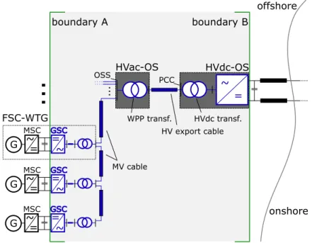
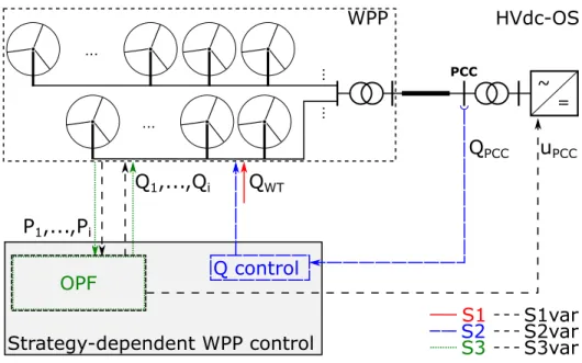
A possible HVdc–connected WPP system is shown in Figure 1 [29]. The full–scale converter (FSC) of the WTs comprises a machine–side converter (MSC) in back–to–back (B2B) arrangement with a grid–side converter (GSC) system. The GSC connects to the low–voltage (LV)–side of the WT trans-former through a coupling inductance and a harmonic filter. A number of WTs is interconnected by medium–voltage (MV) submarine cables to form a string and interface the high–voltage ac offshore substation (HVac–OS). Here, high–voltage (HV) transformer(s) step up the voltage from MV to HV. The HVac–OS is linked to the high–voltage dc offshore substation (HVdc–OS) by HVac submarine cable(s). The HVdc–OS consists of the HVdc trans-former(s), possible harmonic filter(s) and the offshore VSC–HVdc. The off-shore VSC–HVdc station links to any dc–capable interface via submarine dc cables, in the usual execution a point–to–point connection to an onshore VSC–HVdc to connect to the main ac grid.
2.1. Calculation of relevant losses
In general, there are multiple electrical losses occurring in the operation of generators, converters, filters, transformers and cables. For the steady–state power flow analysis, lines, filters and transformers are modeled as lumped circuits (π–models) [31]. In a π–model, the series admittance between two nodes 1 and 2 is defined as:
boundary A boundary B G MSC GSC ~ = =~ FSC-WTG HVac-OS HVdc-OS offshore onshore = ~ WPP transf. HVdc transf. HV export cable MV cable
...
... G MSC GSC ~ = =~ G MSC GSC ~ = =~ PCC OSSFigure 1: Typical arrangement of an HVdc–connected offshore WPP and system bound-aries for loss assessment.
y12=g12+j·b12 = r12 r2 12+x212 −j x12 r2 12+x212 (1) where g12 and b12 are the series conductance and susceptance between the nodes 1 and 2, respectively, and r12 and x12 represent the series resistance and reactance, respectively.
The shunt admittance is calculated as:
ysh 1 =y sh 2 =g sh+j ·bsh (2)
When considering power cables and lines the shunt conductance is very small (gsh ≈ 0) and can be neglected. Values for the series resistance r12, series
reactancex12and shunt susceptancebshare chosen according to manufacturer
(load losses) in the windings having the reactance x12. The iron/core losses (no–load) due the magnetizing current can be represented by a shunt element. The active power imbalance or loss ∆p can be calculated using (3) and the reactive power imbalance ∆q composed of the reactive power generation by the shunt susceptance and reactive power loss is described in (4):
∆p=g12·(u21+u22−2u1u2cosθ12) (3)
∆q =−bsh·(u21+u22)−b12·(u21+u22−2u1u2cosθ12) (4)
where u1 and u2 are the voltages of node 1 and 2, respectively, and θ12 =
θ1 −θ2 is the phase angle difference between the two nodes.
The compilation of losses is limited to the boundaries of the offshore grid as shown in Figure 1: boundary A is the interface between dc link of the GSCs and boundary B is the dc terminal the offshore VSC–HVdc. These boundaries are set following that the reactive power control at the ac terminal of a VSC is independent from the dc–side [3]. Therefore, the control of reactive power at the GSC does not cause additional currents (or losses) in the dc link, the MSC or even the generator. This is also valid for the offshore VSC–HVdc with respect to the HVdc interface. However, the injection of active and reactive power, Pc and Qc, respectively, influences the converter current Ic according to (5): Ic= p P2 c +Q2c √ 3·ULL,rms (5)
The switching and conduction losses Ploss
conv of a VSC might be
approx-imated by a quadratic polynomial function in dependence of the converter currentIc, considering three parts [32]: constant, linear and quadratic losses.
Pconvloss = " a+b· Ic Ir +c· Ic Ir 2# ·Sn (6)
where Ir is the rated converter current, Sn represents the nominal apparent power.
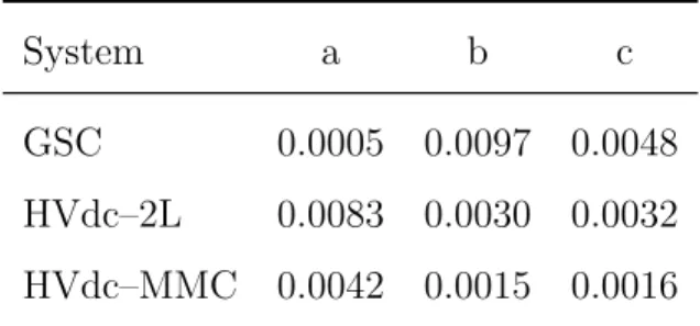
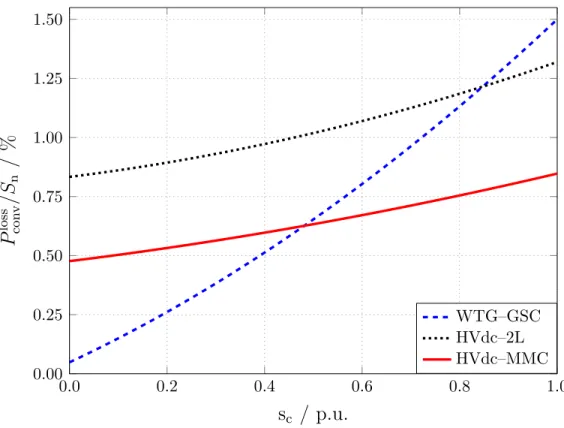
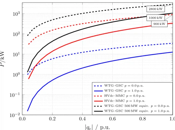
Typical loss data for a system rated to Udc = ±300 kV, Sn = 600 MVA based on a two–level VSC–HVdc (HVdc–2L) can be found in [33]. For a mod-ular multi–level VSC–HVdc (HVdc–MMC) the current–dependent losses in the converter valves are approximately halved compared to a HVdc–2L [34]. Figure 2 shows the relative power losses of the considered power convert-ers deploying (6) with the parameter values from Table 1. The effect of the absolute loss increase due to a reactive power exchange in comparison to exclusively active power injection is represented in Figure 3. The addi-tional converter losses in the HVdc–MMC are up to 0.9 MW when operated at p = 0 p.u. and q = 1 p.u.. For q = 1 p.u., an equally scaled GSC system causes a value of 1 MW additional losses at full power and up to 2.8 MW additional losses for p= 0 p.u..
Table 1: Typical converter loss parameter values used in [32, 33, 34].
System a b c
GSC 0.0005 0.0097 0.0048 HVdc–2L 0.0083 0.0030 0.0032 HVdc–MMC 0.0042 0.0015 0.0016
0.0 0.2 0.4 0.6 0.8 1.0 0.00 0.25 0.50 0.75 1.00 1.25 1.50
sc
/ p.u.
P
loss con v/
S
n/
%
WTG–GSC HVdc–2L HVdc–MMCFigure 2: Relative losses of VSC systems based on their technology and power output.
2.2. Reactive power allocation strategies
The reactive power allocation strategies considered in this paper focus on the normal operation of the HVdc–connected WPP. During system dis-turbances (e.g. under or over–voltage events) each converter would oper-ate based on a predefined control procedure usually according to the GC. Nonetheless, local reactive power limitations due to the availability and PQ capability curve of the WT have to be respected.
In principle, two conventional strategies might emerge to control reactive power in an HVdc–connected WPP when the control variable are limited to be the reactive power set–points:
0.0 0.2 0.4 0.6 0.8 1.0 10−2 10−1 100 101 102 103 900 kW 1000 kW 2800 kW
|
q
c|
/ p
.
u
.
P
/
kW
WTG–GSCp= 0.0 p.u. WTG–GSCp= 1.0 p.u. HVdc–MMCp= 0.0 p.u. HVdc–MMCp= 1.0 p.u. WTG–GSC 500 MW equiv.p= 0.0 p.u. WTG–GSC 500 MW equiv.p= 1.0 p.u.Figure 3: Absolute increase of losses caused by the reactive power injection of VSCs. GSC rating: Sn = 6.67 MVA, cosϕ= 0.9,uac = 0.9 kV; HVdc–MMC Sn = 555.6 MVA, cosϕ= 0.9,uac = 333 kV (udc =±320 kV, modulation index: m= 0.85); GSC 500 MW equivalent to compare with the VSC–HVdc.
1. Strategy 1 (S1): Each GSC operates locally with zero reactive power injection, thusQi = 0 Mvar. This is equal to a unity power factor (PF) operation of the GSCs for Pi 6= 0 MW.
2. Strategy 2 (S2): The VSC–HVdc aims to operate with zero reactive power injection (QPCC = 0 Mvar) by adjusting remotely the reactive power set–points Qi of the WTs. The VSC–HVdc is operated at a unity PF for PPCC 6= 0 MW.
Furthermore, the optimization–based strategy as presented in [22] is consid-ered:
3. Strategy 3 (S3): An optimization algorithm aims to maximize the power output of the system and calculates reactive power set–points for the GSCs according to the actual operating point of the complete system.
The strategies S1 to S3 are studied with a fixed PCC voltage reference of
uPCC = 1 p.u. which is continuously controlled by the VSC–HVdc. Finally, the three initial strategies are extended by the varying voltage reference and introduced as variable strategies:
4. Variable strategy 1 (S1var): Optimization–based with the PCC voltage magnitudeuPCC as control variable whereas the WT injectQi = 0 Mvar (i∈NWT).
5. Variable strategy 2 (S2var): Optimization–based with the PCC voltage magnitude uPCC as control variable and a unique set–point for Qi of the WTs.
6. Variable strategy 3 (S3var): Optimization–based similar to S3 adjust-ing the individual reactive power set–points for the GSCs as well as the PCC voltage magnitude uPCC controlled by the offshore VSC–HVdc. Strategy S1var to S3var allow a variable PCC voltage set–point within the continuous voltage operation boundaries. For all strategies, the VSC– HVdc injects or absorbs the active and reactive power to fulfill the power imbalance equations (acting as a reference bus).
Regarding data exchange requirements, the implementation of S1 does not necessarily use the communication system between the local WT control
and the central WPP control. In contrast, S2 deploys a closed–loop control to adjust the set–pointsQi controlling the measuredQPCC to the reference of 0 Mvar. The reactive power set–point for S1, S2, S1var and S2var is the same for all WTs. The strategies S3, S1var, S2var and S3var necessarily require a communication system as either inputs (active power measurements, opera-tion status of WTs) and outputs (reactive power set–points, uPCC set–point in case of the variable strategies) have to be transfered between WT control and central WPP control.
HVdc-OS ... = ~ ... ... WPP OPF Strategy-dependent WPP control Q1,...,Qi P1,...,Pi Q control QPCC S2 S1 PCC ... S3 S1var uPCC QWT S2var S3var
Figure 4: Schematic of control concepts and communication paths for each strategy.
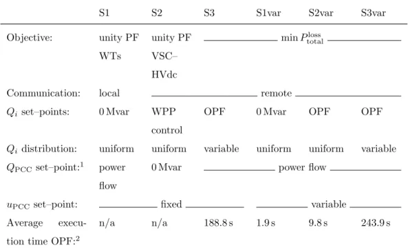
Figure 4 sketches the communication and measurement needs for the presented strategies. To sum up, the six strategies and their characteristics are listed in Table 2.
Table 2: Overview of considered reactive power allocation strategies.
S1 S2 S3 S1var S2var S3var
Objective: unity PF WTs unity PF VSC– HVdc minPloss total
Communication: local remote
Qi set–points: 0 Mvar WPP control
OPF 0 Mvar OPF OPF
Qi distribution: uniform uniform variable uniform uniform variable
QPCC set–point:1 power
flow
0 Mvar power flow
uPCC set–point: fixed variable
Average execu-tion time OPF:2
n/a n/a 188.8 s 1.9 s 9.8 s 243.9 s
2.3. Formulation of the optimization problem
The total active power losses Ploss
total in the system are calculated as:
Ptotalloss =X
∀i
PGSCiloss +Pgridloss+PVSC–HVdcloss . (7) wherePloss
grid are the total losses in the system including collection grid, export
cable(s) and transformer(s), Ploss
GSCi reflects the GSC losses and PVSC–HVdcloss
represents the losses of the HVdc converter.
1The reactive power at the PCC is determined by the power flow in the offshore grid. 2Data is given for the case study performed in this paper.
The design vector x accommodates the voltage set–point uPCC and the reactive power set–points qi of the GSCs:
x=huPCC, q1, q2, . . . , qi
iT
i∈NWT (8)
where NWT is a vector of all WT elements. The optimization problem is
stated as follows:
Minimize f(x) =Ptotalloss(x) (9)
s.t. :
Power flow equations (10)
uk,min ≤uk(x)≤uk,max, k ∈Nbus (11)
|il(x)| ≤il,max, l∈Nbranch (12)
qPCC,min ≤qPCC(x)≤qPCC,max (13)
uPCC∈[uPCC,min, uPCC,max] (14)
qi ∈[qi,min,qi,max], i∈NWT (15)
where Nbus and Nbranch are vectors of all buses (except PCC bus) and
branches, respectively. The voltages uk(x) at the buses Nbus are limited
to the minimum and maximum voltages uk,min and uk,max being a
devi-ation of ±10 % of the nominal voltage. The current in a branch il(x)
represents the highest absolute value of the current at both ends of the branch. It is limited to the corresponding rating il,max. The reactive power
limitations at the PCC, qPCC,min and qPCC,max, and for the WTs, qi,min
voltage constraints between the optimization–based strategies (S3, S1var, S2var and S3var) are reflected by uPCC,min = uPCC,max = 1.0 p.u. for S3 and
uPCC,min = 0.9 p.u. and uPCC,max = 1.1 p.u. for S1var to S3var in (14). Strat-egy S1var is further restricted by qi = qi,min = qi,max = 0 p.u. (i ∈ NWT)
in (15). For strategy S2var the reactive power at the PCC is restricted to qPCC = qPCC,min = qPCC,max = 0 p.u. (13) and additionally qi = qj
(i, j ∈ NWT) meaning that all WTs receive an equal reactive power set–
point.
2.4. Implementation of the optimization–based strategies
The implementation of the optimization–based strategies is made by the combination of the Matlab–based power flow solver package Matpower [35] and the fmincon function of the Matlab Optimization Toolbox. For the purpose of this study, lines and transformers are sufficiently modeled as a
π–section model [36]. In Matpower, every GSCi is defined as static
gener-ator Gi connected to a load bus (PQ bus), injecting active power Pi and
reactive power Qi (i∈NWT). The VSC–HVdc, which sets the PCC voltage
reference, is introduced as the reference bus (slack bus). The integration of the converter losses is made sequentially: the GSC losses caused by Qi are considered as real power demand at the corresponding WT load bus whereas the VSC–HVdc and HVdc transformer losses are calculated by (6) after each load flow computation. The fmincon function uses the interior–point al-gorithm. The optimization is deterministic as the interior–point algorithm reaches local minimums. Nevertheless, the solver runs from multiple starting points to increase the number of solutions. Furthermore, the total execution time is limited. The best solution is selected and verified through load flow
calculation afterwards.
2.5. Conceptual implementation in the industrial application
A feasible implementation of the optimization–based strategies might con-sider a variable refresh rate between 5 min to 10 min. The optimization algo-rithm itself might have a maximum execution time (here set to 300 s). The average execution times recored for the case study in this paper are listed in the last row of Table 2. Obviously, the number of the control variables increases the calculation time. For S1var and S2var average calculation times below 10 s are reached (simulations are run on a 3.5 GHz–system with 16 GB RAM). New set–points might be sent as soon as the optimization algorithm ends. Further time requirements are: the communication times for the active power measurements of the WTs and the reference voltage/reactive power set–points, respectively, and the settling time after receiving the new set– points. The communication delays are negligible on the time frame of the proposed controller as modern communication systems in offshore WPPs con-sider refresh rates of a few hundreds of ms [37]. The settling times might be established as required for normal reactive power set–point changes in WPPs (e.g. 30 sec [38]). Fast voltage support to counteract voltage dips acts inde-pendently from this and supersedes the previous reactive power set–points during activation. For the variable strategies, the reference voltage might be changed first and afterwards the reactive power injections by the WTs. Real– time implementation might be improved by either short–term power or wind forecast to offset the time delay [26] or offline calculation of the optimization algorithm.
3. Case study
The analysis made in this paper aims to draw conclusions relied upon realistic data. Therefore, the WPP characteristics were derived from the French 498 MW F´ecamp project [39, 40]. This WPP is planned with 83 individual FSC–WTs with a nameplate capacity of 6 MW each. For the sake of simplicity, it is assumed that each GSC can provide the equivalent reactive power of a PF of cosϕ=±0.9 at full power.
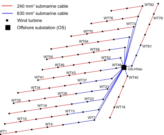
The graphical data offered in [39] allows to estimate individual cable lengths and to define the distribution of the turbines as well as how they are interconnected (visualized in Figure 5). Further relevant reference data, in-cluding component parameters and voltage levels, are provided in Table A.4 in the Appendix. The array cable lengths were calculated according to the distance between the turbines and an additional offset ofl = 100 m to incor-porate the cable routing from the sea bed to the transition piece of the WTs. Table A.5 gives data for the cross–linked polyethylene (XLPE) submarine cables considered in this study.
Contrary to the reference project, the transmission grid connection is adapted to an HVdc connection for the purpose of this paper. Loss data for the offshore VSC–HVdc are calculated according to (6) and Table 1. An HVdc–MMC system is assumed as it presents the state–of–the–art solution in this application [29].
To compute an approximate value of the total energy losses of the WPP, the annual wind speed distribution of the specific site is required. In gen-eral, a Weibull probability distribution approximates the distribution of wind speed for WPP studies. The parameters for the case study are the mean wind
630 mm2 submarine cable
240 mm2 submarine cable
Wind turbine
Offshore substation (OS)
OS-HVac WT40 WT16 WT61 WT79 WT82 WT76 WT70 WT73 WT64 WT55 WT58 WT49 WT52 WT41 WT37 WT34 WT43 WT31 WT28 WT25 WT19 WT22 WT10 WT13 WT1 WT4 WT7 WT46
Figure 5: Layout of the 498 MW F´ecamp reference WPP.
speed of 8.8 m s−1 [40] and a commonly used shape parameter for offshore
locations of 2.2 [6]. The consideration of outages of WTs or the HVdc sys-tem due to maintenance or failure and wake effects is beyond the scope of this study. Thus, the wind speed and active power injection are assumed to be equal for each WT. In order to estimate the monetary value of the total energy losses, the French offshore feed–in tariff of 130eMWh−1 is considered
4. Results
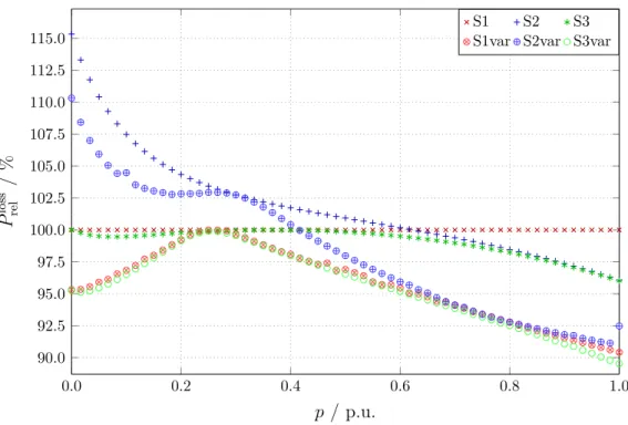
The analysis was performed for the six strategies and active power values ranging from zero to full power (p= 0.0 p.u.to 1.0 p.u.). The first case, S1, is taken as a reference to evaluate the other strategies. The relative loss value shows the increase or reduction of losses for a strategy Sn in comparison to the strategy S1 and is calculated according to:
Prelloss = P loss Sn Ploss S1 ·100 % (16)
where n ∈ {1,2,3,1var,2var,3var} is used to compare the strategies to S1. Figure 6 depicts the total relative losses for all strategies according to (16). The results demonstrate that S2 causes higher losses than S1 for 0.0< p <0.6 p.u. and less losses for p >0.6 p.u.. Here, it is worth mention-ing that an equal relative loss reduction along the whole power range reflects more valuable absolute loss reductions for higher powers. As expected, the employment of the optimization algorithm in S3 has the lowest loss values over the whole power range within the strategies with a fixed PCC voltage reference. Nevertheless, the difference of the total losses between the best conventional strategy (S1 or S2) for individual active power operating points against S3 is of maximal 0.57 % (at p = 0.63 p.u.). The variable strategies S1var to S3var demonstrate that the PCC voltage as control variable has an important impact on the power losses. Specifically in the higher power range for p > 0.4 p.u. the variable strategy performs better than its fixed voltage reference counterpart (S1var with respect to S1, etc.). It is remarkable that S1var causes a similar result as S3var although the latter uses a more com-plex optimization incorporating the individual reactive power set–points of
the WTs. 0.0 0.2 0.4 0.6 0.8 1.0 90.0 92.5 95.0 97.5 100.0 102.5 105.0 107.5 110.0 112.5 115.0 p / p.u. P loss rel / % S1 S2 S3
S1var S2var S3var
Figure 6: Relative total system losses respective to S1 (set equal to 100 %).
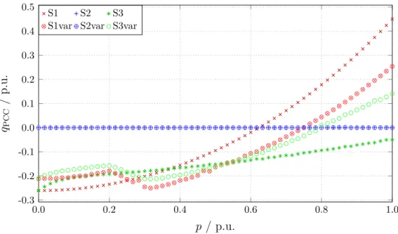
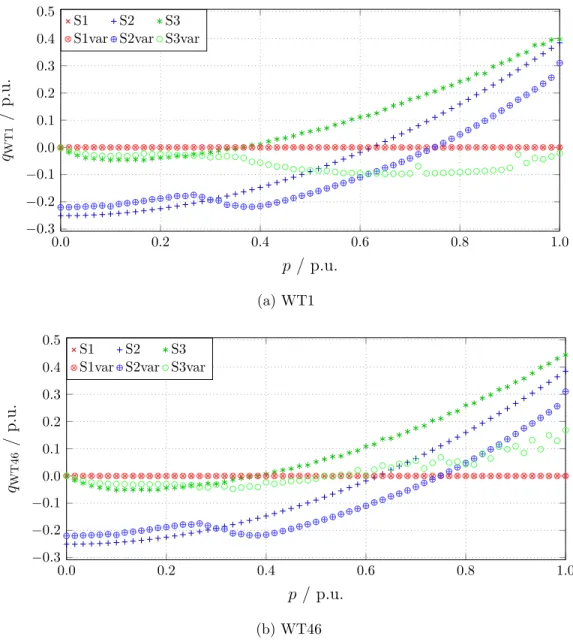
The total amount of consumption and generation of reactive power by transformers, filters and submarine cables in the system has to be balanced by the GSCs and VSC–HVdc. In the following the reactive power injections by the VSC–HVdc qPCC and by two GSCs qWT are presented in Figure 7 and Figure 8 for the whole power range, respectively. For both graphs,
q = 1 p.u. is equal to a PF = 0.9 at full power. The most remote WT from the PCC busbar, WT1, and the closest one, WT46, have been selected for visualization.
The results of S1 indicate that the VSC–HVdc absorbs reactive power for lower powers and injects reactive power for higher powers. Similarly, for
0.0 0.2 0.4 0.6 0.8 1.0 -0.3 -0.2 -0.1 0.0 0.1 0.2 0.3 0.4 0.5 p / p.u. qPCC / p . u . S1 S2 S3
S1var S2var S3var
Figure 7: Reactive power injection by the VSC–HVdc. Positive values correspond to a reactive power injection (capacitive) by the converter.
strategy S2 the reactive powers of the WTs qWT show the same behavior. In both cases, these reactive power sources solely compensate the mentioned amount of reactive power generated in the grid. Thus, the contributions by the VSC–HVdc for strategy S2 as well as by the WTs for strategy S1 are zero as expected. For strategy S1 and S2, respectively, the qWT of WT1 and WT46 are identical due to the uniform set–point distribution for these strategies. For the strategy S3 the set–points for the closest turbine are only up to 0.04 p.u. higher than for the most remote one specifically for active powers higher than p > 0.8 p.u.. For lower active powers the difference is marginal. In fact, the optimization does not result in a significant non– uniform distribution ofqWT set–points. For the optimization-based strategies cases without uniform qi set–points (S3 and S3var) the results in Figure 7
0.0 0.2 0.4 0.6 0.8 1.0 −0.3 −0.2 −0.1 0.0 0.1 0.2 0.3 0.4 0.5 p / p.u. qWT1 / p . u . S1 S2 S3
S1var S2var S3var
(a) WT1 0.0 0.2 0.4 0.6 0.8 1.0 −0.3 −0.2 −0.1 0.0 0.1 0.2 0.3 0.4 0.5 p / p.u. qWT46 / p . u . S1 S2 S3
S1var S2var S3var
(b) WT46
Figure 8: Reactive power injection by (a) the most remote and (b) the closest WT, respectively.
and Figure 8 show the contribution to the total amount of necessary reactive power by the WTs and the VSC–HVdc. Comparing the total reactive power
injection for S3 and S3var results in a lower value for strategy S3var than for S3. This effect is due to the additional variable PCC voltage reference uPCC
in strategy S3var which lowers the reactive power generation in the low power range by decreasing the system voltage. Furthermore, regarding the variation of theqWTset–points for strategy S3var it can be seen that the values for WT1 and WT46 differ for active powers p > 0.6 p.u. whereas WT1 is absorbing reactive power and WT46 is injecting reactive power. This operation of WT1 avoids a local voltage violation due to the higher PCC voltage for this strategy in this power range. Due to its vicinity to the PCC WT46 is not facing this constraint and injects reactive power to compensate. The other variable strategies S1var and S2var lower the reactive power requirement with respect to their counterpart S1 and S2, respectively. This holds true expect for an intermediate power range 0.25 p.u. < p <0.68 p.u.for S1 against S1var whereas 0.3 p.u. < p <0.7 p.u. for S2 versus S2var.
Figure 9 shows the PCC voltage set–point uPCC. For the strategies S1 to S3 the uPCC is fixed at 1.0 p.u.. The variable strategies S1var and S2var result in similar uPCC profiles as S3var. In the lower power range the system voltage is decreased to reduce the reactive power requirements (and related power losses) and the associated power losses in the converters whereas for higher powers the increase of the system voltage leads to lower losses.
The loss distribution in the system appears as component losses of the GSC, the WT transformer and filter, the 33 kV collection grid, the WPP transformers, the HVac export cables and the VSC–HVdc (incl. HVdc transf.). The loss distribution results in Figure 10 and Figure 11 consider the cases where zero or full power is generated, respectively. The power losses
differ-0.0 0.2 0.4 0.6 0.8 1.0 0.90 0.95 1.00 1.05 1.10 p / p.u. uPCC / p . u . S1 S2 S3
S1var S2var S3var
Figure 9: PCC voltage reference set–point imposed by the VSC–HVdc.
ences between the strategies occur mainly in the converters and transformers (no–load losses) for low power (Figure 10) and in the grid components for the full power case (Figure 11). The higher voltage in the offshore grid for S1var to S3var reduces the losses of the grid components in general. From the results for the converter losses for S2 and S2var in the low power scenario it can be concluded that higher losses occur in the GSC and lower losses in the VSC–HVdc compared to the other strategies. Overall, this results in a higher relative loss for strategy S2 compared to S1 in the low power range as depicted in Figure 6.
Figure 12 provides information on voltage values for relevant busbars in the system. The plots use boxplots to display mean, 25 % and 75 % per-centiles as well as minimum and maximum values of the corresponding sets over the whole power range. In Figure 12a the voltage levels are shown
WTG-GSC WTG transf. 33kV grid WPP transf. Exp ort cables VSC–HVdc 0.27 0 .45 1.29 ·10 −3 0.46 4.63 ·10 −3 2.59 0.89 0.52 5.21 ·10 −2 0.49 2.24 ·10 −3 2.39 0.27 0 .45 1.29 ·10 −3 0.46 4.63 ·10 −3 2.59 0.27 0. 37 1.05 ·10 −3 0.37 3.77 ·10 −3 2.55 0.81 0.45 4.57 ·10 −2 0.43 1.96 ·10 −3 2.39 0.27 0. 36 9.53 ·10 −4 0.37 3.68 ·10 −3 2.54 P / MW S1 S2 S3 S4 S1var S2var
Figure 10: Distribution of losses in the system forp= 0.0 p.u..
for strategies S1 to S3 specifically for the busbars of the HV–side of the WT transformers, the LV–side of the WPP transformers, denoted as offshore sub-station (OSS), and the PCC voltage. Figure 12b displays the voltage levels for the variable strategies S1var to S3var. Firstly, the voltages are kept within the admissible voltage limitations for all busbars and strategies. Secondly, it can be seen that the mean voltages for the WTs are higher for S3 compared to S1 and S2 due to the optimization procedure. The variable strategies S1var and S2var explore a wider voltage band compared to their counterparts. For strategy S1var and S3var the voltages of the WTs are almost exclusively close to the upper limit of 1.1 p.u.. Among the fixed reference voltage strategies S1 has the most varying voltage profile at the OSS busbar whereas S2 keeps
WTG-GSC WTG transf. 33kV grid WPP transf. Exp ort cables VSC–HVdc 7.26 6.52 4.53 6.26 0.84 4.66 7.41 5.99 4.13 5.8 0.79 4.59 7.45 5.96 4.11 5.78 0.79 4.6 7.26 5.41 3.63 5.21 0.68 4.63 7.36 5.59 3.81 5.42 0.73 4.6 7.27 5.3 3.55 5.11 0.67 4.61 P / MW S1 S2 S3 S4 S1var S2var
Figure 11: Distribution of losses in the system forp= 1.0 p.u..
its values closely below 1 p.u.. The values for S3 show insignificant variation for this busbar slightly above 1 p.u.. For the variable strategies this busbar voltage correlates with the variable PCC voltage.
Figure 13 depicts the reactive power injections by the GSCs and the VSC– HVdc. Again, Figure 13a displays the results for the fixed voltage strategies whereas Figure 13b contains the results for the variable strategies. Firstly, the plots show that S1 and S2 both cause a uniform reactive power injection by the WTs. The values for S3 (for S3var, respectively) vary from each other and demonstrate the variable distribution of set–points caused by the optimization routine, respectively. For strategy S3, the reactive power values of the GSC are mainly injections which result in a generally higher voltage
in the WPP grid when compared to S1 and S2. In contrast, for strategy S3var the use of a high PCC voltage reference results in a partly inductive operation of the GSCs in order keep the voltage inside the upper limit. This is especially the case for WTs which are very remote to the PCC busbar such as WT1 (see also Figure 8a). Secondly, the variation of the reactive power injection by the VSC–HVdc is the highest for S1 whereas S3 is kept within a moderate range absorbing reactive power. The plot of S2 consequently results to zero reactive power exchange. For strategy S3var the VSC–HVdc operates mainly absorbing reactive power unless for higher powers where it injects reactive power. Contemplating the combination of both the WT and the VSC–HVdc results it is obvious that S3 and S3var reach a sharing of reactive power injection within the WPP. The variable strategies result in less reactive power injection variation than their respective fixed strategies. This is caused by the variable PCC voltage which lowers the reactive power requirements of the converters in the system.
The annual energy loss (AEL) obtained by applying the different strate-gies is displayed in Table 3. For S2 the absolute energy losses are reduced by 696 MWh and for S3 by 2131 MWh compared to strategy S1, respectively. The variable strategies permit a further loss reduction: S1var 6320 MWh, S2var 4224 MWh and S3var 6819 MWh in comparison to S1, respectively. The monetary saving of these additional active power in–feeds is of 90 kefor S2, 277 ke for S3 and oscillates between 549 ke and 886 ke for the variable strategies, respectively.
WT1–83 (S1) WT1–83 (S2) WT1–83 (S3) 0.90 0.95 1.00 1.05 1.10 u / p . u . OSS PCC (a)
WT1–83 (S1var) WT1–83 (S2var) WT1–83 (S3var) 0.90 0.95 1.00 1.05 1.10 u / p . u . OSS PCC (b)
Figure 12: Voltage distribution of (a) fixed reference voltage strategies and (b) variable reference voltage strategies. The boxplots show mean, 25 %–, 75 %–percentiles, minimum and maximum values. The HV–side busbars of the WT transformers, the LV–side of the WPP transformer (OSS) and the PCC busbar are displayed.
5. Conclusions and recommendations
This work presented reactive power and voltage control concepts to op-erate HVdc–connected WPPs aiming to minimize overall system losses. The
WT1–83 (S1) WT1–83 (S2) WT1–83 (S3) −0.3 −0.2 −0.1 0.0 0.1 0.2 0.3 0.4 0.5 q / p . u . VSC–HVdc (a)
WT1–83 (S1var) WT1–83 (S2var) WT1–83 (S3var) −0.3 −0.2 −0.1 0.0 0.1 0.2 0.3 0.4 0.5 q / p . u . VSC–HVdc (b)
Figure 13: Reactive power injections of (a) fixed reference voltage strategies and (b) variable reference voltage strategies. The boxplots show mean, 25 %–, 75 %–percentiles, minimum and maximum values. All GSC and VSC–HVdc reactive power injections are plotted. A positive value expresses to a reactive power injection (capacitive).
WT reactive power set–points and the PCC reference voltage imposed by the offshore VSC–HVdc are calculated to gain minimal losses in the system by
Table 3: AEL and the monetary equivalent (ME) thereof.
S1 S2 S3 S1var S2var S3var
AEL/ GWh 94.54 93.84 92.41 88.22 90.3 87.72
ME / Meyr−1 12.29 12.20 12.01 11.47 11.74 11.40
means of an optimization–based algorithm. First, a loss assessment has been conducted for such HVdc–connected WPPs where the collection grid and converter losses of the VSC–HVdc as well as of the WTs are considered. A case study for a 500 MW–sized reference WPP was performed for the whole active power range to draw conclusions for six different reactive power con-trol concepts. From the results it was concluded that the optimization–based reactive power control contributes to a reduction of energy losses by up to 4 % for a fixed PCC voltage and up to 10 % with the incorporation of a variable PCC voltage set–point in comparison to unity PF operation of the WTs. Moreover, it was found that in case of the conventional reactive power allocation strategies the application of a single reactive power injection re-sponsibility for either GSCs or the VSC–HVdc is not optimal considering the whole power range. Consequently, the use of an optimization–based algorithm results in a share of the reactive power injection responsibility between the WT and the VSC–HVdc. The application of the variable strate-gies S1var, S2var or S3var result in lower losses and mostly lower reactive power injections at the expense of a wider usage of the continuous voltage operation band. The deployment of the variable strategy might cause the system to operate continuously at its voltage limits which might inherently
violate them if the system operating point changes. This drawback might be counteracted with an additional security margin on the voltage limits in the optimization algorithm. The results of the optimization–based controllers motivate the implementation of such into the central WPP control. Fur-thermore, the involved parties in the system which are generally the offshore transmission asset owner (HVdc system owner) and the WPP owner could share the additional benefits of a calculated 886 keannual cost reduction for the 500 MW case study performed in this paper.
Acknowledgements
The research leading to these results has received funding from the People Programme (Marie Curie Actions) of the European Unions Seventh Frame-work Programme (FP7/2007-2013) under REA grant agreement number 317221, project title MEDOW. Any opinions, findings, and conclusions or recom-mendations expressed in this material are those of the authors and do not necessarily reflect those of General Electric
Table A.4: Reference data and relevant system parameter. WT grid connection Nominal voltage (Uac/kV) 0.9 GSC (Sn/MVA, cosϕ) 6.67,±0.9 Coupling impedance (r/p.u.,x/p.u.) 0.004, 0.13 MV transformer (LV/HV, Sn/MVA, r/p.u.,x/p.u.,no–load losses/p.u.) 0.9/33, 6.7, 0.009, 0.06, 0.0008 MV collection grid Nominal voltage (Uac/kV) 33 Total cable length (l/km) 118
Total number of turbines 83
HV transformer (N, LV/HV, Sn/MVA,
r/p.u.,x/p.u.,no–load losses/p.u.)
2, 33/220, 280, 0.003, 0.15, 0.0004
HVac export cable
Nominal voltage (Uac/kV) 220 Export cable(s) (N,A/mm2,l/km) 2, 800, 10
HVdc transmission
Nominal voltages (Uac/kV,Udc/kV) 333,±320
Converter (topology,Sn/MVA, cosϕ) HVdc–MMC, 555.6,±0.9 Table A.5: Data for XLPE submarine cables [42, 43, 44].
Ur / kV A / mm2 Ir / A R0 / Ω km −1 L0 / mH km−1 C0 / µF km−1 33 240 581 0.098 0.36 0.23 33 630 904 0.041 0.31 0.34 220 800 830 0.032 0.40 0.17
References
[1] European Wind Energy Association (EWEA), The European offshore wind industry - key trends and statistics 2015, Tech. Rep. February (2016).
[2] H. Polinder, J. A. Ferreira, B. B. Jensen, A. B. Abrahamsen, K. Atal-lah, R. A. McMahon, Trends in wind turbine generator systems, IEEE J. Emerg. Sel. Top. Power Electron. 1 (3) (2013) 174–185. doi:10.1109/JESTPE.2013.2280428.
[3] A. Yazdani, R. Iravani, Voltage-Sourced Converters in Power Sys-tems, John Wiley and Sons, Inc., Hoboken, NJ, USA, 2010. doi:10.1002/9780470551578.
[4] Alstom Grid, HVDC-VSC: transmission technology of the future, Think Grid (8) (2011) 13–17.
URL http://www.gegridsolutions.com/alstomenergy/grid/grid/
news-and-events/thinkgrid/index.html
[5] ENTSO-E, Requirements for grid connection applicable to all genera-tors, Tech. Rep. March (2013).
[6] Carbon Trust, Offshore wind power: big challenge, big opportunity, Tech. rep. (2008).
URL http://www.carbontrust.com/media/42162/
ctc743-offshore-wind-power.pdf
[7] O. Gomis-Bellmunt, A. Junyent-Ferr´e, A. Sumper, S. Galceran-Arellano, Maximum generation power evaluation of variable frequency offshore
wind farms when connected to a single power converter, Appl. Energy 87 (10) (2010) 3103–3109. doi:10.1016/j.apenergy.2010.04.025.
[8] J. L. Dom´ınguez-Garc´ıa, D. J. Rogers, C. E. Ugalde-Loo, J. Liang, O. Gomis-Bellmunt, Effect of non-standard operating frequencies on the economic cost of offshore AC networks, Renew. Energy 44 (2012) 267–280. doi:10.1016/j.renene.2012.01.093.
[9] M. de Prada Gil, O. Gomis-Bellmunt, A. Sumper, Technical and eco-nomic assessment of offshore wind power plants based on variable fre-quency operation of clusters with a single power converter, Appl. Energy 125 (2014) 218–229. doi:10.1016/j.apenergy.2014.03.031.
[10] M. De Prada Gil, J. Dom´ınguez-Garc´ıa, F. D´ıaz-Gonz´alez, M. Arag¨ u´es-Pe˜nalba, O. Gomis-Bellmunt, Feasibility analysis of offshore wind power plants with DC collection grid, Renew. Energy 78 (2015) 467–477. doi:10.1016/j.renene.2015.01.042.
[11] J. Park, K. H. Law, Layout optimization for maximizing wind farm power production using sequential convex programming, Appl. Energy 151 (2015) 320–334. doi:10.1016/j.apenergy.2015.03.139.
[12] M. De-Prada-Gil, C. G. Al´ıas, O. Gomis-Bellmunt, A. Sumper,
Maximum wind power plant generation by reducing the
wake effect, Energy Convers. Manag. 101 (2015) 73–84. doi:10.1016/j.enconman.2015.05.035.
for voltage control applications, Renew. Energy 29 (3) (2004) 377–392. doi:10.1016/S0960-1481(03)00224-6.
[14] G. Tapia, A. Tapia, J. X. Ostolaza, Proportional-integral regulator-based approach to wind farm reactive power management for secondary voltage control, IEEE Trans. Energy Convers. 22 (2) (2007) 488–498. doi:10.1109/TEC.2005.858058.
[15] L. Meegahapola, S. Durairaj, D. Flynn, B. Fox, Coordinated utilisation of wind farm reactive power capability for system loss optimisation, Eur. Trans. Electr. Power 21 (1) (2011) 40–51. doi:10.1002/etep.410.
[16] L. G. Meegahapola, E. Vittal, A. Keane, D. Flynn, Voltage security constrained reactive power optimization incorporating wind generation, in: 2012 IEEE Int. Conf. Power Syst. Technol. POWERCON 2012, 2012, pp. 1–6. doi:10.1109/PowerCon.2012.6401436.
[17] H. Van Pham, I. Erlich, J. L. Rueda, Probabilistic evaluation of volt-age and reactive power control methods of wind generators in dis-tribution networks, IET Renew. Power Gener. 9 (3) (2015) 195–206. doi:10.1049/iet-rpg.2014.0028.
[18] R. G. de Almeida, E. D. Castronuovo, J. A. Pe¸cas Lopes, Opti-mum generation control in wind parks when carrying out system operator requests, IEEE Trans. Power Syst. 21 (2) (2006) 718–725. doi:10.1109/TPWRS.2005.861996.
[19] M. Wilch, V. S. Pappala, S. N. Singh, I. Erlich, Reactive power generation by DFIG based wind farms with AC grid
connec-tion, in: Power Tech, 2007 IEEE Lausanne, 2007, pp. 626–632. doi:10.1109/PCT.2007.4538389.
[20] M. Martinez-Rojas, A. Sumper, O. Gomis-Bellmunt, A. Sudri`a-Andreu, Reactive power dispatch in wind farms using particle swarm optimiza-tion technique and feasible soluoptimiza-tions search, Appl. Energy 88 (12) (2011) 4678–4686. doi:10.1016/j.apenergy.2011.06.010.
[21] B. Zhang, W. Hu, P. Hou, Z. Chen, Reactive power dispatch for loss minimization of a doubly fed induction generator based wind farm, in: 2014 17th Int. Conf. Electr. Mach. Syst., 2014, pp. 1373–1378. doi:10.1109/ICEMS.2014.7013688.
[22] K. Sch¨onleber, S. Rat´es-Palau, M. De-Prada-Gil, O. Gomis-Bellmunt, Reactive power optimization in HVDC-connected wind power plants considering wake effects, in: U. Betancourt, T. Ackermann (Eds.), 14th Wind Integr. Work., Energynautics GmbH, Brussels, 2015.
[23] M. Montilla-DJesus, D. Santos-Martin, S. Arnaltes, E. D. Castron-uovo, Optimal reactive power allocation in an offshore wind farms with LCC-HVdc link connection, Renew. Energy 40 (1) (2012) 157–166. doi:10.1016/j.renene.2011.09.021.
[24] V. S. Pappala, M. Wilch, S. N. Singh, I. Erlich, Reactive power manage-ment in offshore wind farms by adaptive PSO, in: 2007 Int. Conf. Intell. Syst. Appl. to Power Syst. ISAP, 2007. doi:10.1109/ISAP.2007.4441595. [25] H. V. Pham, J. L. Rueda, I. Erlich, Online optimal control of reactive
sources in wind power plants, IEEE Trans. Sustain. Energy 5 (2) (2014) 608–616. doi:10.1109/TSTE.2013.2272586.
[26] I. Erlich, W. Nakawiro, M. Martinez, Optimal dispatch of reactive sources in wind farms, in: 2011 IEEE Power Energy Soc. Gen. Meet., 2011, pp. 1–7. doi:10.1109/PES.2011.6039534.
[27] V. S. Pappala, W. Nakawiro, I. Erlich, Predictive optimal control of wind farm reactive sources, in: 2010 IEEE PES Transm. Dis-trib. Conf. Expo. Smart Solut. a Chang. World, 2010, pp. 1–7. doi:10.1109/TDC.2010.5484587.
[28] B. Zhang, P. Hou, W. Hu, M. Soltani, C. Chen, Z. Chen, A Reac-tive Power Dispatch Strategy With Loss Minimization for a DFIG-Based Wind Farm, IEEE Trans. Sustain. Energy 7 (3) (2016) 914–923. doi:10.1109/TSTE.2015.2509647.
[29] CIGRE Working Group B4.55, HVDC connection of offshore wind power plants, Tech. rep., CIGRE (may 2015).
[30] CIGRE Working Group B3.36, Special considerations for AC collector systems and substations associated with HVDC - connected wind power plants, Tech. rep., CIGRE (mar 2015).
[31] G. Andersson, Power system analysis, Lecture 227-0526-00, ITET ETH Z¨urich, 2012.
[32] H. Polinder, F. Van Der Pijl, G.-J. De Vilder, P. Tavner, Com-parison of Direct-Drive and Geared Generator Concepts for Wind
Turbines, IEEE Trans. Energy Convers. 21 (3) (2006) 725–733. doi:10.1109/TEC.2006.875476.
[33] G. Daelemans, K. Srivastava, M. Reza, S. Cole, R. Belmans, Mini-mization of steady-state losses in meshed networks using VSC HVDC, in: 2009 IEEE Power Energy Soc. Gen. Meet., IEEE, 2009, pp. 1–5. doi:10.1109/PES.2009.5275450.
[34] U. N. Gnanarathna, A. M. Gole, A. D. Rajapakse, S. K. Chaudhary, Loss estimation of modular multi-level converters using electro-magnetic transients simulation, in: Int. Conf. Power Syst. Transients, Delft, 2011, pp. 2–7.
[35] R. D. Zimmerman, C. E. Murillo-Sanchez, R. J. Thomas, MATPOWER: steady-state operations, planning, and analysis tools for power systems research and education, IEEE Trans. Power Syst. 26 (1) (2011) 12–19. doi:10.1109/TPWRS.2010.2051168.
[36] R. D. Zimmerman, C. E. Murillo-Sanchez, Matpower 5.1 user’s manual (2015).
[37] A. Pettener, SCADA and communication networks for large scale off-shore wind power systems, in: IET Conf. Renew. Power Gener. (RPG 2011), IET, 2011, pp. 11–11. doi:10.1049/cp.2011.0101.
[38] TenneT TSO GmbH, Requirements for offshore grid connections in the grid of TenneT TSO GmbH, Tech. Rep. December, Tennet (2012).
[39] ´Eoliennes Offshore des Hautes Falaises, Projet de parc ´eolien au large de F´ecamp, Tech. rep., Dossier du Maitre d’Ouvrage (Project Management Report) (2013).
URL http://www.parc-eolien-en-mer-de-fecamp.fr
[40] Parc ´eolien en mer de F´ecamp, ´Etude de la ressource en vent, Tech. rep. (2011).
URL http://www.parc-eolien-en-mer-de-fecamp.fr
[41] French Government, Arrˆet´e du 17 novembre 2008 fixant les conditions d’achat de l’´electricit´e produite par les installations utilisant l’´energie m´ecanique du vent, Tech. rep. (2008).
[42] Nexans, 2XS(FL)2YRAA RM 19/33 (36)kV cable datasheets for differ-ent cross-sections (2014).
URL http://www.nexans.de
[43] ABB, XLPE submarine cable systems rev. 5 (2010).
URL http://www.abb.com/cables
[44] Nkt Cables, High voltage cable systems - cables and accessories up to 550 kV, Tech. rep. (2012).