Randomization Inference and Sensitivity
Analysis for Composite Null Hypotheses with
Binary Outcomes in Matched Observational
Studies
To appear in the
Journal of the American Statistical Association:
Theory and Methods
Colin B. Fogarty
Pixu Shi
Mark E. Mikkelsen
Dylan S. Small
∗Abstract
We present methods for conducting hypothesis testing and sensitivity analyses for composite null hypotheses in matched observational studies when outcomes are binary. Causal estimands discussed include the causal risk difference, causal risk ratio, and the effect ratio. We show that inference under the assumption of no unmeasured confound-ing can be performed by solvconfound-ing an integer linear program, while inference allowconfound-ing for unmeasured confounding of a given strength requires solving an integer quadratic program. Through simulation studies and data examples, we demonstrate that our formulation allows these problems to be solved in an expedient manner even for large data sets and for large strata. We further exhibit that through our formulation, one can assess the impact of various assumptions on the potential outcomes on the performed inference. R scripts are provided that implement our methodology.
Keywords: Causal Inference; Sensitivity Analysis; Integer Programming; Causal Risk;
Effect Ratio
∗Colin B. Fogarty is Doctoral Candidate, Department of Statistics, Wharton School, University of
Penn-sylvania, Philadelphia PA 19104 (e-mail: [email protected]). Pixu Shi is Doctoral Candidate, Center for Clinical Epidemiology and Biostatistics, Perelman School of Medicine, University of Pennsylvania, Philadelphia, PA 19104. Mark E. Mikkelsen is Assistant Professor, Pulmonary, Allergy and Critical Care Division and Center for Clinical Epidemiology and Biostatistics, Perelman School of Medicine, University of Pennsylvania, Philadelphia, PA 19104. Dylan S. Small is Professor, Department of Statistics, Wharton School, University of Pennsylvania, Philadelphia PA 19104.
1
Introduction
1.1
Challenges for Matched Observational Studies with
Bi-nary Outcomes
Matching is a simple, transparent and convincing way to adjust for overt biases in an observational study. In a study employing matching, treated subjects are placed into strata with control subjects on the basis of their observed covariates. In each stratum, there is either one treated unit and one or more similar control units, or one control unit and one or more similar treated units (Hansen, 2004; Rosenbaum, 2010; Stuart, 2010). The overall covariate balance between the two groups is then assessed with respect to the produced stratification, and inference is only allowed to proceed if the balance is deemed acceptable. This procedure encourages researcher blinding, as both the construction of matched sets and the assessment of balance proceed without ever looking at the outcome of interest just as they would in a blocked randomized trial.
Despite our best efforts, observational data can never achieve their randomized experimental ideal as the assignment of interventions was conducted outside of the re-searcher’s control. Nonetheless, randomization inference provides an appealing frame-work within which to operate for matched observational studies. The analysis initially proceeds as though the data arose from a blocked randomized experiment, with the strata constructed through matching now regarded as existing before random ment occurred. Randomization inference uses only the assumption of random assign-ment of interventions to provide a “reasoned basis for inference” in a randomized study (Fisher, 1935). In the associated sensitivity analysis for an observational study, de-partures from random assignment of treatment within each block due to unmeasured confounders are considered. The sensitivity analysis forces the practitioner to explic-itly acknowledge greater uncertainty about causal effects than would be present in a randomized experiment due to the possibility that unmeasured confounders affect treatment assignment and the outcome (Rosenbaum, 2002b, Section 4).
With binary outcomes, randomization inference and sensitivity analyses in matched observational studies raise computational challenges that have heretofore limited their use. When the outcome is continuous rather than binary and an additive treatment ef-fect is plausible, hypothesis testing and sensitivity analyses for the treatment efef-fect can be conducted for asimple null hypothesis, and confidence intervals can then be found by inverting a series of such tests. This is a straightforward task, since the potential outcomes under treatment and control for each individual are uniquely determined by the hypothesized treatment effect (Hodges and Lehmann, 1963). Inference under no unmeasured confounding merely requires a simple randomization test, and a sensitivity analysis can be performed with ease through the asymptotically separable algorithm of Gastwirth et al. (2000). When dealing with binary responses, however, an additive treatment effect model is inapplicable: if an effect exists it is most likely heterogeneous, as the intervention may cause an event for one individual while not causing the event for another. As such, confidence intervals are instead constructed for causal estimands whose corresponding hypothesis tests arecomposite in nature, meaning there are many allocations of potential outcomes which yield the same hypothesized value of the causal estimand; see Rosenbaum (2001, 2002a) for further discussion. To reject a null hypoth-esis for a causal parameter of this sort, we must reject the null for all values of the
potential outcomes which satisfy the null. The situation is further complicated when conducting a sensitivity analysis, as inference must also account for the existence of an unmeasured confounder with a range of impacts on the assignment of interventions within a matched set. We now illustrate these points by investigating the causal effect of one post-hospitalization protocol versus another after an acute care stay on hospital readmission rates.
1.2
Motivating Example: Effect of Post-Acute Care
Pro-tocols on Hospital Readmission
At the time of discharge after an acute care hospitalization, a fundamental question arises: to where should the patient be discharged? The long-term goal shared by providers and patients envisions a transition home and a return to normalcy, yet a pre-mature discharge home without appropriate guidance could impede a durable recovery. An important measure of whether a patient has achieved a durable recovery is whether the patient does not need to be readmitted to the hospital within a certain period of time. Different avenues for reducing rehospitalization rates have recently gar-nered significant attention nationwide (Jencks et al., 2009), and post-acute care is one mechanism through which hospital readmission rates may be improved (Ottenbacher et al., 2014). For individuals who are not gravely ill, post-acute care entails more inten-sive discharge options than a simple discharge home without further supervision such as discharge home while receiving visits from skilled nurses, physical therapy, and other additional health benefits (referred to henceforth as “home with home health services”); or discharge to an acute rehabilitation center. Post-acute care use is on the rise in the United States; however, post-acute care services can be quite costly, sometimes even rivaling the cost of a hospital readmission (Mechanic, 2014). It is thus of interest to assess the relative merits of various post-acute care protocols for reducing hospital readmission rates.
We aim to assess the causal effect of being discharged to an acute rehabilitation center versus home with home health services on hospital readmission rates through a retrospective observational study. Hospital records for acute medical and surgical pa-tients discharged from three hospitals in the University of Pennsylvania Hospital system between 2010 and 2012 were collected; see Jones et al. (2015) for more details on this study. Within this data set, there are 4893 individuals assigned to acute rehabilitation and 35,174 individuals assigned to home with home health services, for 40,067 total individuals. We would like to assess whether discharge to acute rehabilitation reduces the causal risk of hospital readmission relative to discharge home with home health ser-vices. Beyond testing this hypothesis, we would also like to create confidence intervals for causal parameters that effectively summarize the impact of discharge location on hospital readmission rates in our study population. Two causal estimands of interest for this comparison are thecausal risk difference, which is the difference in proportions of readmitted patients if all patients had been assigned to acute rehabilitation versus that if all patients had been discharged home with home health services; and thecausal
risk ratio, which is the ratio of these two proportions.
Through the use of matching with a variable number of controls (Ming and Rosen-baum, 2000), individuals assigned to acute rehabilitation were placed in matched sets with varying numbers of home with home health services individuals (ranging from 1 to
20) who were similar on the basis of their observed covariates. We used rank-based Ma-halanobis distance with a propensity score caliper (estimated by logistic regression) of 0.2 as our distance metric to perform the matching. We further required exact balance on the indicator of admission to an intensive care unit to better control for whether an individual had a critical illness. In Appendix A, we demonstrate that this stratification resulted in acceptable balance on the basis of the standardized differences between the groups.
In the stratified experiment that our match aims to mimic, randomization inference can be readily used to test Fisher’s sharp null of no effect. Under Fisher’s sharp null, the unobserved potential outcomes are assumed to equal the observed potential outcomes for each individual. The sharp null can then be assessed by noting that within each stratum, the number of treated individuals for whom an event is observed follows a hypergeometric distribution. The total number of treated individuals with events across all strata is then distributed as the sum of independent hypergeometric distributions, forming the basis for what has become known as the Mantel-Haenszel test (Mantel and Haenszel, 1959; Rosenbaum, 2002b).
Testing a null on the causal risk difference or the causal risk ratio presents challenges not encountered when testing the sharp null, as many allocations of potential outcomes could yield the same causal parameter. For example, if we are testing the null that the causal risk difference is 0, the allocation under Fisher’s null is merely one of many choices (i.e., it is merely one element of the composite null). Conducting a hypothesis test and performing a sensitivity analysis requires assessing tail probabilities for all elements of the composite null, both under the assumption of no unmeasured confounding and while allowing for an unmeasured confounder of a range of strengths. Direct enumeration of all possible combinations of potential outcomes is computationally infeasible for even moderate sample sizes. In our motivating example, there are 240,067 possible combinations of potential outcomes, evenwithoutconsidering values for the unmeasured confounder.
We instead aim to find the combination of potential outcomes and unmeasured confounders that results in the worst-casep-value for the test being conducted. If the null hypothesis corresponding to this worst-case allocation can be rejected, we can then reject all elements of the composite null. Rosenbaum (2002a) uses a similar approach for inference on theattributable effect, which is the effect of the treatment on the treated individuals. There it is shown that under the assumption of a nonnegative treatment effect (i.e., the treatment may cause an event, but does not preclude an event from happening if it would have happened under the control) a simple enumerative algorithm yields an asymptotic approximation worst-case p-value for this composite null. This is because the impact on thep-value by attributing a given outcome to the treatment can be well approximated through asymptotic separability (Gastwirth et al., 2000), such that one can satisfy the null while finding the worst-case allocation by sorting the strata on the basis of their impact on thep-value and attributing the proper number of effects by proceeding down the sorted list. Recent works by Yang et al. (2014) and Keele et al. (2014) discuss how the attributable effect can also be used to define estimands of interest in instrumental variable studies. See Appendix B for further discussion on estimands which focus on the treatment effect on the treated versus the treatment effect on the entire study population.
the treatment’s effect on treated individuals (the risk difference and risk ratio being two such estimands), and even for estimands focusing on the treated individuals but not assuming a known direction of effect, finding the worst-case allocation does not simplify in the same manner. This is because finding the potential outcome allocation with the largest impact on the p-value on a stratum-wise basis does not readily yield an allocation that satisfies the composite null. The problem is not separable on a stratum-wise basic even asymptotically, as the requirement that the composite null must be true necessarily links the strata together in a complex manner. There are two non-complementary forces at play in the required optimization problem: for some strata, the potential outcome allocations should maximize the impact on the p-value, while in other strata the missing potential outcome allocations should work towards satisfying the composite null. For our motivating example, there are over 300,000 types of contributions to thep-value that must be considered in the sensitivity analysis when we do not assume a known direction of effect (as is shown in Section 6.1). Explicit enumeration is intractable here, as we must consider which allowed combinations of these contributions maximize thep-value while satisfying the null in question. As such, a different approach is required to make the computation feasible.
1.3
Integer Programming as a Path Forward
In this paper, we show that hypothesis testing for a composite null with binary out-comes can be performed by solving an integer linear program under the assumption of no unmeasured confounding. When conducting a sensitivity analysis by allowing for unmeasured confounding of a certain strength, an integer quadratic program is re-quired. These optimization problems yield the worst-casep-value within the composite null so long as a normal approximation to the test statistic is justified. We show that our formulation is strong, in that the optimal objective value for our integer program closely approximates that of the corresponding continuous relaxation. As we demon-strate through simulation studies and real data examples, this allows hypothesis testing and sensitivity analyses to be conducted efficiently even with large sample sizes despite the fact that integer programming is N P-hard in general, as discrete optimization solvers heavily utilize continuous relaxations in their search path. Through comparing our formulation to an equivalent binary program in the supplementary material, we also demonstrate that recent advances in optimization software (Jünger et al., 2009) alone are not sufficient for solving the problem presented herein; rather, a thought-ful formulation remains essential for solving large-scale discrete optimization problems expeditiously.
2
Causal Inference after Matching
2.1
Notation for a Stratified Randomized Experiment
Suppose there are I independent strata, the ith of which contains ni ≥ 2
individ-uals, that were formed on the basis of pre-treatment covariates. In each stratum,
mi individuals receive the treatment and ni−mi individuals receive the control, and
min{mi, ni−mi}= 1. We proceed under the stable unit treatment value assumption
one unit is not affected by the treatment assignment of other units; and (2) there are no hidden levels of the assigned treatment, meaning tha tthe treatments for all individuals with the same level of observed treatment are truly comparable (Rubin, 1986). LetZij
be an indicator variable that takes the value 1 if individual j in stratum iis assigned to the treatment. Each individual has two sets of binary potential outcomes, one un-der treatment, {rT ij, dT ij} and one under control, {rCij, dCij}. rT ij and rCij are the
primary outcomes of interest, while dT ij and dCij are indicators of whether or not an
individual would actually take the treatment when randomly assigned to the treatment or control group. The observations for each individual areRij =rT ijZij+rCij(1−Zij)
andDij =dT ijZij+dCij(1−Zij); see Neyman (1923) and Rubin (1974) for more on the
potential outcomes framework. In the classical experimental setting, dT ij −dCij = 1
∀i, j, and hence all individuals take the administered treatment. For a randomized encouragement design, (Holland, 1988), Zij represents the encouragement to take the
treatment (which is randomly assigned to patients), whiledT ij anddCij are the actual
treatment received if Zij = 1 and Zij = 0 respectively. Matched observational studies
assuming strong ignorability (Rosenbaum and Rubin, 1983) aim to replicate a classi-cal stratified experiment, whereas matched studies employing an instrumental variable strive towards a randomized encouragement design, with Zij being the instrumental
variable.
There are N = PI
i=1ni total individuals in the study. Each individual has
ob-served covariates xij and unobserved covariate uij. Let R = [R11, R12, ...,, RInI]
T,
Ri = [Ri1, ..., Rini]
T, and let the analogous definitions hold for D,D
i, Z,Zi. Let
rT = [rT11, ..., rT InI], rT i = [rT i1, ..., rT ini], and let the analogous definitions hold for
the other potential outcomes and the unobserved covariate. LetX be a matrix whose rows are the vectorsxij. Finally, letΩbe the set ofQIi=1ni possible values ofZunder
the given stratification. In a randomized experiment, randomness is modeled through the assignment vector; eachz∈Ωhas probability1/|Ω|of being selected. Hence, quan-tities dependent on the assignment vector such as Z, R and D are random, whereas
F = {rT,rC,dT,dC,X,u} contains fixed quantities. For a randomized experiment,
P(Zij = 1|F,Z∈Ω) =mi/ni, andP(Z=z|F,Z∈Ω) = 1/|Ω|, where the notation|B|
denotes the number of elements in the setB.
2.2
Conducting a Sensitivity Analysis
In an observational study, theIstrata are still generated based on pre-treatment covari-ates, but are only created after treatment assignment has taken place. Furthermore, the treatment assignment was conducted outside of the practitioner’s control, which may introduce bias due to the existence of unmeasured confounders. We follow the model for a sensitivity analysis of Rosenbaum (2002b, Section 4), which states that fail-ure to account for unobserved covariates may result in biased treatment assignments within a stratum. This model can be parameterized by a number Γ = exp(γ) ≥ 1
which bounds the extent to which the odds ratio of assignment can vary between two individuals in the same matched stratum. Letting πij = P(Zij = 1|F), we can
write the allowed deviation as 1/Γ ≤ πij(1−πik)/(πik(1−πij)) ≤ Γ. This model
can be equivalently expressed in terms of the observed covariates xij and the
unob-served covariate uij (assumed without loss of generality to be between 0 and 1), as
log (πij/(1−πij)) = ζ(xij) +γuij, where ζ(xij) = ζ(xik), i = 1, ..., I,1 ≤ j, k ≤ ni.
models. The probabilities of each possible allocation of treatment and control are given by P(Z= z|F,Z∈ Ω) = exp(γzTu)/P
b∈Ωexp(γbTu), where u = [u11, u12, ..., uI,ni].
If Γ = 1, the distribution of treatment assignments corresponds to the randomization distribution discussed in Section 2.1. For Γ>1, the resulting distribution differs from that of a randomized experiment with the extent of the departure controlled byΓ.
Consider a simple hypothesis test based on a test statistic of the form T = ZTq, whereq =q(rT,rC,dT,dC) is a permutation invariant, arrangement increasing
func-tion. Most commonly employed statistics are of this form; see Rosenbaum (2002b, Section 2.4) for a detailed discussion. Without loss of generality reorder the elements of q such that within each stratum qi1 ≤qi2 ≤ .. ≤ qini. For a given value of Γ and
for fixed values of the potential outcomes, a sensitivity analysis proceeds by finding tight upper and lower bounds on the upper tail probability, P(T ≥ t), by finding the worst-case allocation of the unmeasured confounder u. One then finds the value of Γ
such that the conclusions of the study would be materially altered. The more robust a given study is to unmeasured confounding, the larger the value of Γ must be to alter its findings.
As is demonstrated in Rosenbaum and Krieger (1990) for strata with mi = 1, for
each Γ an upper bound on P(T ≥ t) is found at a value of the unobserved covariate
u+ ∈ U+
1 ×...×U+I, where U
+
i consists of ni −1 ordered binary vectors (each of
length ni) with 0 =u+i1 ≤ u+i2...≤ u+ini = 1. Similarly, a lower bound on P(T ≥ t) is
found at a vector u− ∈ U−1 ×...×U−I with 1 =u−i1 ≥ u−i2...≥u−in
i = 0. Under mild
regularity conditions on q, T is well approximated by a normal distribution. Large sample bounds on the tail probability can be expressed in terms of corresponding bounds on standardized deviates. These results can readily extended to stratifications yielded by a full match through a simple redefinition ofZandq; see Rosenbaum (2002b, Section 4, Problem 12).
3
Composite Null Hypotheses
3.1
Estimands of Interest
To motivate our discussion, we will focus on three causal estimands of interest with binary outcomes. Note however that the general framework for inference and sensitivity analyses presented herein can be applied to any causal estimand for binary potential outcomes with an associated test statistic that can be written as ZTq for a function
q(·)that satisfies the conditions outlined in Section 2.2. The causal parameters we will consider are the causal risk difference, causal risk ratio, and the effect ratio, defined as:
Risk Difference δ := 1 N I X i=1 ni X j=1 (rT ij−rCij) Risk Ratio ϕ:= PI i=1 Pni j=1rT ij PI i=1 Pni j=1rCij Effect Ratio λ:= PI i=1 Pni j=1(rT ij−rCij) PI i=1 Pni j=1(dT ij−dCij) .
As mentioned in the introduction, the causal risk difference measures the difference in proportions of observed events had all the individuals received the treatment and observed events had all individuals received the control. Similarly, the causal risk ra-tio measures the rara-tio of these two proporra-tions. Each of these estimands has merits and shortcomings relative to the other, owing to the fact that the risk difference mea-sures an effect on an absolute scale while the risk ratio meamea-sures an effect on a relative scale; see Appendix C for further discussion of these two measures. These estimands are appropriate under strong ignorability (Rosenbaum and Rubin, 1983); in the corre-sponding idealized experiment, there are simply treated and control individuals, and all individuals comply with their assigned treatment regimen.
The effect ratio is a ratio of two average treatment effects, and hence serves as an assessment of the relative magnitude of the two treatment effects (Baiocchi et al., 2010; Yang et al., 2014). It is a causal estimand of interest in instrumental variable studies. In the idealized experiment being mimicked, Zij represents the randomized
encouragement to take the treatment or control, whiledT ij and dCij indicate whether
the treatment would be taken if Zij = 1 and Zij = 0 respectively. The effect ratio
then represents the ratio of the effect of the encouragement on the outcome to the effect of the encouragement on the treatment received. If the encouragement (1) is truly randomly assigned within strata defined by the observed covariates; and (2) can only impact the outcome of an individual if the encouragement changes the individual’s choice of treatment regimen (the exclusion restriction: dT ij =dCij ⇒ rT ij = rCij), Z
is then an instrument for the impact of the treatment on the response (Angrist et al., 1996). The parameter λ still has an interpretation in terms of relative magnitude of the two effects even if the exclusion restriction is not met, but the exclusion restriction coupled with monotonicity (dT ij ≥dCij, also referred to as assuming “no defiers”) give
λ an additional interpretation as the average treatment effect among individuals who
arecompliers, i.e. individuals for whichdT ij−dCij; this is commonly referred to as the
local average treatment effect. While we will not always assume monotonicty holds, we
will make the assumption that the encouragement has anaggregate positive effect, i.e.
PI
i=1
Pni
j=1dT ij−dCij >0, such that the effect ratio is well defined.
3.2
Testing a Composite Null
Note first that a null hypothesis onδ, ϕ, orλcorresponds to a composite null hypothesis on the values of the potential outcomes, as multiple potential outcome allocations yield the same value for the causal parameter. Let Θ(rT,rC,dT,dC) be a function that
maps a given set of potential outcomes to the corresponding causal parameter value of interest,θ. We call a set of potential outcomes {rT,rC,dT,dC} consistent with a null
hypothesisH0 :θ=θ0 for a causal parameterθif the following conditions are satisfied:
(A1) Consistency with observed data: ZijrT ij+ (1−Zij)rCij = Rij; ZijdT ij + (1−
Zij)dCij =Dij
(A2) Consistency with assumptions made on potential outcomes (A3) Agreement with the null hypothesis: Θ(rT,rC,dT,dC) =θ0
The first condition recognizes that we know the true values for half of the potential out-comes based on the observed data. The second condition means that if the practitioner has made additional assumptions on the potential outcomes, those assumptions must
be satisfied in the allocations of potential outcomes under consideration. Assumptions could include a known direction of effect, monotonicity, the exclusion restriction, and combinations thereof. The third condition signifies that when testing a null hypothesis, we must only consider allocations of potential outcomes where the corresponding causal parameter takes on the desired value.
LetH(θ0)represent the set of potential outcomes satisfying conditions A1 - A3. As
the size of a composite null hypothesis test is the supremum of the sizes of the elements of the composite null, to reject the null H0 : θ = θ0 at level α, we must reject the
null for all {rT,rC,dT,dC} ∈ H(θ0) at level α. As direct enumeration of H(θ0) is a
laborious (and likely computationally infeasible) task, we instead aim to find a single worst-case allocation{rT,rC,dT,dC}∗ such that rejection of{rT,rC,dT,dC}∗ at level
α implies rejection for all{rT,rC,dT,dC} ∈ H(θ0).
We consider test statistics of the form T(θ0) = PiI=1Ti(θ0) with expectation 0
under the null atΓ = 1. Letψ(θ0;rT i,rCi,dT i,dCi) =E[Ti(θ0)]. Thus,PiI=1ψ(θ0;rT i,
rCi,dT i,dCi) = 0 if and only if Θ(rT,rC,dT,dC) = θ0. For our three estimands of
interest, the stratum-wise contributions to the test statistic are
Ti(δ0) =−niδ0+ni ni X j=1 (ZijRij/mi−(1−Zij)Rij/(ni−mi)) Ti(ϕ0) =ni ni X j=1 (ZijRij/mi−ϕ0(1−Zij)Rij/(ni−mi)) Ti(λ0) =ni ni X j=1 (Zij(Rij−λ0Dij)/mi−(1−Zij)(Rij −λ0Dij)/(ni−mi)),
with respective stratum-wise expectations
ψ(δ0;rT i,rCi,dT i,dCi) =−niδ0+ ni X j=1 (rT ij−rCij) ψ(ϕ0;rT i,rCi,dT i,dCi) = ni X j=1 (rT ij−ϕ0rCij) ψ(λ0;rT i,rCi,dT i,dCi) = ni X j=1 (rT ij−λ0dT ij−(rCij−λ0dCij)).
To express these statistics in the required form for conducting a sensitivity analysis, defineZ˜ such thatZ˜ij =Zij if mi = 1 and Z˜ij = 1−Zij if mi >1. Ifmi = 1, define
q(·) as: (q(δ0;rT i,rCi,dT i,dCi))j =ni −δ0+rT ij/mi− X k6=j rCik/(ni−mi) (q(ϕ0;rT i,rCi,dT i,dCi))j =ni rT ij/mi− X k6=j ϕ0rCik/(ni−mi) (q(λ0;rT i,rCi,dT i,dCi))j =ni (rT ij−λ0dT ij)/mi− X k6=j (rCik−λ0dCik)/(ni−mi)
The analogous definition holds when mi > 1: simply redefine q(·) within stratum i
such that the proper contribution is given to Ti(·) if unit j in stratum i receives the
control (and thus, all other units receive the treatment). The test statisticZ˜Tq(·)then has the required form for conducting a sensitivity analysis.
Under mild regularity conditions, Lyapunov’s central limit theorem yields that all three of the test statistics T(θ0) under consideration are well approximated by a
nor-mal distribution for Γ ≥1. See Fogarty et al. (2015) for a discussion with regards to the risk difference (the risk ratio follows through similar arguments), and see Baiocchi et al. (2010) for a discussion for the effect ratio. Finding the worst-case allocation
{rT,rC,dT,dC}∗ at a given Γ can be well approximated by finding the allocation of
potential outcomes and unobserved confounder that results in the worst-case standard-ized deviate. While this observation simplifies our task, it alone is not sufficient for making both inference and sensitivity analyses feasible for our estimands of interest; rather, we must exploit other features of the optimization problem.
4
Symmetric Tables
We now introduce the required framework and notation for our optimization problem. Though many equivalent formulations are possible, the one we describe has a decision variable for each unique distribution on a stratum’s contribution to the test statistic. This is an extension of the formulation of Fogarty et al. (2015), which was catered towards maximizing the variance of the estimated causal risk difference under no un-measured confounding. In Section 5.3, we discuss the elements of our formulation which facilitate solving the corresponding integer program efficiently.
Let Tzrd
i ={j :Zij =z, Rij =r, Dij =d},(z, r, d)∈ {0,1}3,i∈ {1, ..., I}, denote
the eight possible partitions of indices of individuals in stratumiinto sets based on their value of the encouraged treatment, observed response, and taken treatment. Within each set, all members share the same value of eitherrT ij or rCij, and of eitherdT ij or
dCij. For example, if j, k∈ Ti011, thenrCij =rCik=dCij =dCik = 1, yet the values of
rT ij, rT ik, dT ij, dT ik are unknown. Note that for the stratifications under consideration
P
(r,d)∈{0,1}2|Ti0rd|=ni−mi,
P
(r,d)∈{0,1}2|Ti1rd|=mi, and the minimum of these two
quantities is always 1. |Tzrd
i | can be thought of as the value in cell (z, r, d) of a 23
factorial table that counts the number of individuals with each combination of(z, r, d)
in stratumi.
Under no assumption on the structure of the potential outcomes, there are 22ni
possible sets of potential outcomes in stratum ithat are consistent with the observed data, each of which results in a particular distribution for the contribution to the test statistic from stratum i, Ti(θ0). Fortunately, one need never consider all 22ni
allocations. First, without any assumptions on the potential outcomes, the22nipossible
sets of potential outcomes in stratum i only yield Q
(z,r,d)∈{0,1}3(|Tizrd|+ 1)2 unique
distributions for Ti(θ0). To see this, note that the test statistics under consideration
are permutation invariant within each stratum. Let us examine the set T000
i as an
illustration. Here, we have dCij = rCij = 0 for all j ∈ Ti000. Of the 2|T
000
i | pairings
[rT ij, rCij], there are only |Ti000|+ 1non-exchangeable allocations of values for {rT ij :
j ∈ T000
i }: (0,0...,0),(1,0, ...,0), ..., and (1,1, ...,1). Analogous argument shows that
there are only |T000
i |+ 1 non-exchangeable arrangements for dT ij, thus resulting in
(|T000
of(|Tzrd
i |+ 1)2 for each of the other seven partitions.
Additional structure is often imposed on the potential outcomes on top of con-sistency with the observed data. For example, in the classical experiment we have thatdT ij−dCij = 1∀i, j, meaning that all patients comply with their assigned
treat-ment. Hence, the four partitions where Zi −Di 6= 0 are empty, and in the
remain-ing partitions dT ij and dCij are fixed at 1 and 0 respectively. This results in only
Q
(z,r)∈{0,1}2(|Tizrz|+ 1) allowed non-exchangeable allocations within stratum i; note
the lack of a square in the expression. This is also shown in Rigdon and Hudgens (2015, Section 3). Other assumptions such as a known direction of effect, monotonic-ity, and the exclusion restriction can be seen to similarly reduce the set of allowed non-exchangeable allocations.
It would seem as though we must consider at mostQI
i=1
Q
(z,r,d)∈{0,1}3(|Tizrd|+ 1)2
different distributions for T(θ0) = PiI=1Ti(θ0) in our optimization problem.
Fortu-nately, note first that we assume independence between strata, and further note that we are using a normal approximation to conduct inference. Hence, both the expecta-tions and variances sum between strata and we do not need to consider covariances between strata. Further, in the same way that there were a limited number of non-exchangeable allocations of potential outcomes in each stratum due to repetition, many observed23 factorial tables in the data are repeated multiple times. For example, the matching with multiple controls performed on the data in our motivating example from Section 1 returned 4893 strata, of which only 234 were unique.
4.1
Expectation, Variance, and Null Deviation
We now introduce the requisite notation to exploit these facts to facilitate inference. Let Ci = (|Ti000|, ..., |Ti111|) be the observed counts of the 23 tables for stratum i. C={C1, ...,CI}is a (multi)set, where the number of unique elements equals the number of unique 23 tables observed in the data, which will typically be much less than its
dimension. Let S be the number of unique tables, and let s ∈ {1, ..., S} index the unique tables. Define I(i) to be a function returning the index of the unique table corresponding to the table observed in stratum i. Hence, I(i) = I(`) if and only if
Ci=C`. LetMs=|I−1(s)|be the number of strata where unique tableswas observed,
and let n˜s = nb for any b ∈ I−1(s) be the number of observations in unique table
s. Finally, let Ps be the number of allowed non-exchangeable potential outcomes for
unique tables, and let{[rT[sp],rC[sp],dT[sp],dC[sp]]}, p∈ {1, ..., Ps}be the set of allowed
potential outcome allocations that are consistent with unique tables, where tablewise consistency refers to adherence to conditions A2 and A3 within tables.
Without loss of generality, we assume that the observed statistic,tθ0, is larger than
its expectation under the null atΓ = 1, 0. In upper bounding the upper tail probability
P(T(θ0)≥tθ0), we thus restrict our search to the set of unobserved confoundersu
+∈
U+ as discussed in Section 2.2. The analogous procedure would hold for u− ∈U− if
tθ0 <0.
For the sth unique table, and the pth set of allowed potential outcome allocations consistent within tables,s∈ {1, ..., S},p∈ {1, .., Ps}, form
q(θ0)[sp]j = (q(θ0;rT[sp],rC[sp],dT[sp],dC[sp]))j. Reorder theq(θ0)[sp]jsuch thatq(θ0)[sp]1 ≤
a∈ {1, ...n˜s−1}, as µ(θ0)[sp]a= Pa j=1q(θ0)[sp]j + Γ Pn˜s j=a+1q(θ0)[sp]j a+ Γ(˜ns−a) , (1) and ν(θ0)[sp]a= Pa j=1(q(θ0)[sp]j)2+ Γ P˜ns j=a+1(q(θ0)[sp]j)2 a+ Γ(˜ns−a) −(µ(θ0)[sp]a)2. (2)
This notation is reminiscent of that of Gastwirth et al. (2000). The index a corre-sponds to the the vector of unmeasured confounders u+ with a zeroes followed by
˜
ns−a ones. µ(θ0)[sp]a and ν(θ0)[sp]a represent the expectation and variance of the
contribution to the test statistic T(θ0) from a matched set with observed table s,
consistent set of potential outcomes p, and allocation of unmeasured confounders a. Let µθ0 = [µ(θ0)[11]1, ..., µ(θ0)[SPS],˜nS−1], and let νθ0 = [ν(θ0)[11]1, ..., ν(θ0)[SPS],n˜S−1].
Finally, recalling the definition ofψ(·)from Section 3 as the expectation of the contri-bution to the test statisticT(θ0)from stratumi, defineψ(θ0)[sp]j = (ψ(θ0;rT[sp],rC[sp],
dT[sp],dC[sp]))j, and defineψθ0 = [ψ(θ0)[11]1, ..., ψ(θ0)[SPS],n˜S−1].
5
Inference and Sensitivity Analysis
Letx[sp]abe an integer variable denoting how many times the set of potential outcomes
p that is consistent with unique table s with allocation of unmeasured confounders
a is observed in the data, s ∈ {1, ..., S}, p ∈ {1, ..., Ps}, a ∈ {1, ...,n˜s−1}, and let
x= [x[11]1, .., x[SPs],n˜S−1]. For a givenθ0being tested,µ(θ0)[sp]ax[sp]aandν(θ0)[sp]ax[sp]a
represent the contribution to the overall mean and variance of the test statistic if thepth
set of potential outcomes in unique tableswith allocation of unmeasured confounders
a is observed x[sp]a times, and µTθ
0x and ν
T
θ0x represent the overall expectation and
variance across all unique tables, potential outcomes and unmeasured confounders.
PPs
p=1
P˜ns−1
a=1 x[sp]a then represents how many times the sth unique table was observed
in the data, a number which we defined to beMs. Hence, PPp=1s
P˜ns−1
a=1 x[sp]a=Ms.
Note that through our formulation we have restricted optimization to the set of observations that adhere to conditions A1 (consistency with the observed data) and A2 (consistency with any other assumptions made by the modeler on the potential outcomes) of Section 3.2. We enforce condition A3 (that the null must be true in the resulting allocation of potential outcomes) through adding a linear constraint to our optimization problem: ψTθ0x= 0. The following integer program facilitates hypothesis testing and confidence interval construction under no unmeasured confounding (Section 5.1), as well as a sensitivity analysis for any Γ>1(Section 5.2).
minimize x (tθ0 −µ T θ0x) 2−κ(νT θ0x) (P1) subject to Ps X p=1 ˜ ns−1 X a=1 x[sp]a=Ms ∀s ψTθ0x= 0 x[sp]a∈Z ∀s, p, a x[sp]a≥0 ∀s, p, a
whereZ are the integers and κ > 0 is a positive constant to be described. The above
formulation is sufficient for tests on the risk difference and risk ratio. For the effect ratio, we can impose the constraint of an aggregate positive effect of the intervention,
PI
i=1
Pni
j=1dT ij−dCij >0, through an additional linear inequality.
5.1
Hypothesis Testing and Confidence Intervals Under No
Unmeasured Confounding
For conducting inference under pure randomization (that is, underΓ = 1), the value of
µT
θ0xis fixed to the expectation of the test statistic under the null, 0. Hence,(tθ0−µ
T θ0x)
is constant as well, and (P1) reduces to an integer linear program. This program is equivalent to finding the largest variance over all feasible x. Call the optimal vector
x∗θ
0, and call the corresponding maximal variance ν
T θ0x
∗
θ0. The worst-case deviate for
testingθ=θ0 can then be found by setting zθ0 =tθ0/ q
νT θ0x
∗
θ0.
To form a 100×(1−α)% confidence interval at Γ = 1, we simply invert a se-ries of tests. Explicitly, we find upper and lower bounds, θu and θ`, such that θ` =
SOLVE n θ:tθ/ q νθTx∗θ =z1−α/2 o and θu = SOLVE n θ:tθ/ q νθTx∗θ=zα/2 o , where
zq is the q quantile of a standard normal distribution. These endpoints can be found
through a grid search over θ, or by using the bisection algorithm.
5.2
Sensitivity Analysis through Iterative Optimization
ForΓ>1, (P1) is instead an integer quadratic program. First, note that we reject the null with a two-sided alternative at sizeαif(tθ0−µ
T θ0x)
2/(νT
θ0x)≥χ
2
1,1−αfor all values
of the potential outcomes that are consistent with the null being tested, where χ2 1,1−α
is the1−αquantile of aχ21 distribution. Equivalently, we need only determine whether
(tθ0 −µ
T θ0x)
2 −χ2
1,1−α(νθT0x) ≥ 0 for all feasible x. This can be done by minimizing
(P1) with κ = χ2
1,1−α over all feasible x, and checking whether or not the objective
value atx∗θ
0 is greater than zero.
One may also be interested in knowing the worst-case deviate itself (equivalently, the worst-casep-value), rather than simply knowing the result of the test. The optimal vectorx∗θ0 for (P1) atκ=χ21,1−αneed not result in the worst-case deviate; however, we
now show that we can find the worst-casep-value through an iterative procedure based on (P1). To proceed, we find the value κ =κ∗ such that the minimal objective value of (P1) equals 0. As is proved in Dinkelbach (1967), such a value of κ∗ exactly equals the minimal squared deviate. Interpreted statistically, the value κ∗ is the maximal critical value for the squared deviate such that the null could be still be rejected, which is equivalent to the value of the deviate itself. Although finding this zero could be performed using a grid search, we instead solve for the optimal x∗θ
0 through the
following algorithm.
1. Start with an initial value κ(0).
2. In iteration i≥1, set κ=κ(i−1) in (P1).
3. Solve the resulting program, and set κ(i) = (tθ0 −(µ
T θ0x ∗(i) θ0 )) 2/(νT θ0x ∗(i) θ0 ).
4. If κ(i) =κ(i−1) terminate the algorithm: setx∗θ
0 =x
∗(i)
θ0 , and setκ
5. Otherwise, return to step 2. Repeat until convergence.
Note that the sequence{κ(i)}is bounded below by 0. It is also monotone decreasing for
i≥1, as (tθ0 −µ T θ0x ∗(i+1) θ0 ) 2−κ(i)(νT θ0x ∗(i+1) θ0 ) ≤(tθ0 −µ T θ0x ∗(i) θ0 ) 2−κ(i)(νT θ0x ∗(i) θ0 ) = 0, which impliesκ(i)≥(tθ0 −(µ T θ0x ∗(i+1)))2/(νT θ0x ∗(i+1) θ0 ) =κ
(i+1). Hence, this algorithm
will converge to a stationary point κ∗. In practice, we find that this is achieved very quickly, frequently within 2 or 3 steps. At κ∗, note that it must be the case that the objective value in (P1) equals 0. This means that at the termination of the iterative procedure, we have converged to the minimal deviate. The maximal p-value is then
Φ(−√κ∗) for a one-sided test or 2×Φ(−√κ∗) for a two-sided test, where Φ(·) is the
CDF of a standard normal distribution.
5.3
Computation Time
In the past, researchers have been dissuaded from suggesting methodology that requires the solution of an integer program, as problems of this sort are N P-hard in general. In this section, we present simulation studies to assuage fears that our integer linear (Γ = 1) and quadratic (Γ > 1) programs may have excessive computational burden. Before doing so, we discuss two properties of an integer programming formulation that substantially influence the performance of integer programming solvers: the strength of the corresponding continuous relaxation, and the avoidance of symmetric feasible solutions (Bertsimas and Tsitsiklis, 1997).
A strong formulation of an integer program is one for which the polyhedron defined by the constraint set, P = {x : Ax ≤ b,x ∈ R}, is close to the integer hull, PI =
Conv{x :x∈ P ∩Z}. In an ideal world, the integer hull and the relaxed polyhedron
would align, meaning that any linear programming relaxation would be guaranteed to have an integral optimal solution since any linear program has an optimal solution at the vertex of its corresponding polyhedron. For a quadratic program, havingPI=P does not guarantee coincidence of the true and relaxed optimal solutions, as a quadratic program may have a solution at an edge. Nonetheless, having P far from PI can hamper the progress of a mixed integer programming solver, as it increases the number of cuts required by branch-and-cut algorithms to strengthen the continuous relaxation (Mitchell, 2002).
A symmetric formulation is one in which variables can be permuted without chang-ing the structure of the problem. Formulations of this sort can also cripple standard integer programming solvers even with modest problem size. This is due in large part to the generation of isomorphic solution paths by bound and branch-and-cut algorithms, which in turn complicates the process by which a given node is proven optimal or suboptimal. Although methods exist to detect symmetry groups in a given formulation, formulations that explicitly avoid such groups are strongly preferred; see Margot (2010) for a discussion of these points.
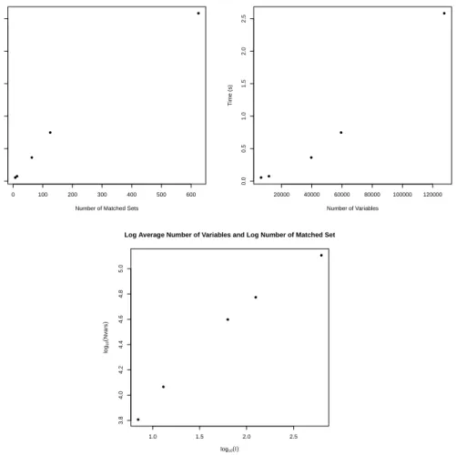
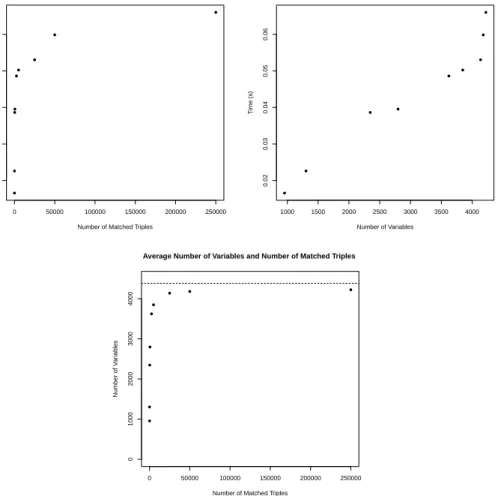
We now present simulation studies to demonstrate that neither weakness nor sym-metry of formulation proves inimical to conducting hypothesis testing and sensitivity analyses using the methodology outlined in this paper, even with large data sets and large stratum sizes. In our first setting, in each of 1000 iterations we sample 1250 matched sets from the strata in our motivating example from Section 1.2. We assign treated individuals and control indivduals an outcome of 1 with probability 0.75 and 0.25 respectively. Each iteration thus has strata ranging in size from 2 to 21, and each
data set has an average of roughly 10,000 individuals within it. Large strata affect computation time, as they result in larger numbers of non-exchangeable potential out-come allocations within a stratum and fewer duplicated 2×2 tables in the data. In our data set, 25% of the matched strata had one acute rehabilitation individual and 20 home with home health services patients. This simulation setting thus produces particularly challenging optimization problems: on average, each iteration had 170,000 variables over which to optimize. As we demonstrate in Appendix D, the number of variables, itself affected by the number and size of the unique observed tables, is a primary determinant of computation time for the optimization routine.
We conduct two hypothesis tests in each iteration: a null on the causal risk differ-ence, δ= 0.2, and on the causal risk ratio, ϕ= 1.75. For both of the causal estimands being assessed, we test the stated nulls with two-sided alternatives atΓ = 1(no unmea-sured confounders, integer linear program) andΓ = 3(unmeasured confounding exists, integer quadratic program). We record the required computation time for each data set, which includes both the time taken to define the necessary constants for the problem and also the time required to solve the optimization problem. To measure the strength of our formulation, we also recorded whether or not the initial continuous relaxation had an optimal solution which was itself integral, and if not the relative difference in optimal objective function values between the integer and continuous formulations (defined to be the absolute difference of the two, divided by the absolute value of the relaxed value). Simulations were conducted on a desktop computer with a 3.40 GHz processor and 16.0 GB RAM. The Rprogramming language was used to formulate the optimization problem, and the R interface to the Gurobi optimization suite was used to solve the optimization problem.
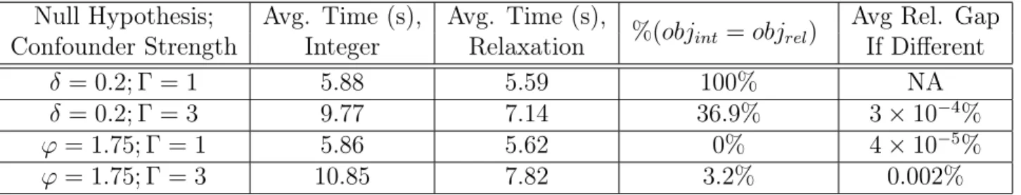
Table 4 shows the results of this simulation study. As one can see, our formulation yields optimal solutions in well under a minute for both the integer linear and integer quadratic formulations despite the magnitude of the problem at hand. The strength of our formulation is further evidenced by the typical discrepancy between the inte-ger optimal solution and that of the continuous relaxation. For testing the causal risk difference, we found that in all of the simulations performed assuming no unmeasured confounding the integer program and its linear relaxation had thesame optimal objec-tive value. When testing at Γ = 3 the quadratic relaxation differed from the integer programming solution in roughly 2/3 of the simulations; however, the resulting average relative gap between the two was a minuscule3×10−4%. For testing the causal risk ra-tio, the objective values tended not to be identically equal atΓ = 1orΓ = 3, which has to do with the existence of fractional values in the row of the constraint matrix enforcing the null hypothesis; nonetheless, the average gap among those iterations where there was a difference was 4×10⁻⁵%for the linear program, and 0.002% for the quadratic program. This suggests not only that we have arrived upon a strong formulation, but that one could in practice accurately approximate (P1) by its continuous relaxation.
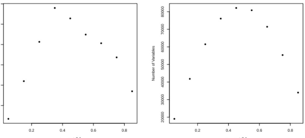
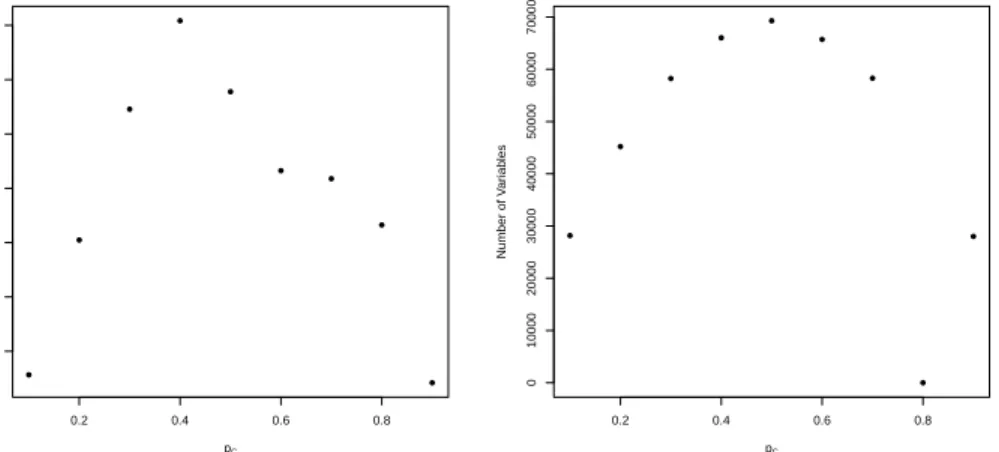
Appendix D contains additional simulation studies which serve not only to further illustrate the strength of our formulation, but also to provide insight into what elements of the problem affect computation time. We present simulations varying the value ofΓ
used, the number of matched sets, the null hypothesis being tested, the magnitude of the true effect, and the prevalence of the outcome under treatment and control in order to assess the impact of each of these factors on the time required to define the required constants and to carry out the optimization. We then compare our formulation to
Table 1: Computation times for tests of δ = 0.2 and ϕ = 1.75 at Γ = 1 (integer linear
program) and Γ = 3 (integer quadratic program), along with percentages of coincidence of
the integer and relaxed objective values, and average gaps between integer solution and the continuous relaxation if a difference existed between the two.
Null Hypothesis; Avg. Time (s), Avg. Time (s),
%(objint =objrel)
Avg Rel. Gap
Confounder Strength Integer Relaxation If Different
δ= 0.2; Γ = 1 5.88 5.59 100% NA
δ= 0.2; Γ = 3 9.77 7.14 36.9% 3×10⁻⁴%
ϕ= 1.75; Γ = 1 5.86 5.62 0% 4×10⁻⁵%
ϕ= 1.75; Γ = 3 10.85 7.82 3.2% 0.002%
an equivalent, but highly symmetric, formulation in order to highlight the importance of avoiding symmetry for achieving a strong formulation with reasonable computation time. Finally, we present a simulation study akin to the one presented in this section but using real data for the outcome variables as opposed to simulated outcomes.
6
Data Examples
We employ our methodology in two data examples. In Section 6.1, we present hypoth-esis testing and a sensitivity analysis for the causal risk difference and causal risk ratio in our motivating example from Section 1, wherein we compare hospital readmission rates for two different post-hospitalization protocols after an acute care hospitalization. In Section 6.2, we reexamine the instrumental variable study of Yang et al. (2014) com-paring mortality rates for premature babies being delivered byc-section versus vaginal births. In addition to inference, confidence intervals, and sensitivity analyses, we also provide point estimators for the causal estimands of interest. These are formed by using our test statistic, T(θ), as an estimating equation for an m-estimator (Van der Vaart, 2000), i.eθˆ:=SOLVE{θ:T(θ) = 0}; see Appendix E for further discussion.
As will be shown, the findings in both of our examples exhibit varying degrees of sensitivity to unmeasured confounding: under the strongest assumptions, we fail to reject the null of no treatment effect after Γ = 1.157 in our first example and after
Γ = 1.67 in our second. To provide context for the levels of robustness possible in a well designed observational study, Section 4.3.2 of Rosenbaum (2002b) notes that the finding of a causal relationship between smoking and lung cancer in Hammond (1964) continued to be significant untilΓ = 6, meaning that an unmeasured confounder would have had to increase the odds of smoking by a factor of six while nearly perfectly predicting lung cancer in order to overturn the study’s finding.
6.1
Risk Difference and Risk Ratio
We now return to our study of the impact of discharge to an acute rehabilitation cen-ter versus to home with home health services on hospital readmission rates afcen-ter an acute care hospitalization. We use sixty day hospital readmission after initial hospital
discharge as our outcome of interest. In terms of counterfactuals, we want to compare sixty day hospital readmission rates if all patients had been sent to acute rehabilita-tion with readmission rates if all patients had been assigned to home with home health services. We define Rij = 1 if an individual was readmitted to the hospital, and 0
otherwise. We let Zij = 1 if an individual was assigned to acute rehabilitation. The
marginal proportions of sixty day hospital readmission after accounting for observed confounders through matching are 0.206 for acute rehabilitation, and 0.243 for home with home health services. We will analyze this data set with and without the assump-tion of a known direcassump-tion of effect. When assuming a direcassump-tion of effect we assume that it is nonpositive in this example, meaning that going to acute rehabilitation can never hurt an individual: an individual who would not be readmitted to the hospital within sixty days after being discharged to home with home health services could not have been readmitted to the hospital within sixty days after being discharged to acute rehabilitation.
The estimated risk difference isδˆ=−0.0369(favoring acute rehabilitation) regard-less of whether we assume a nonpositive treatment effect. We construct confidence intervals by inverting a series of hypothesis tests on{δ0}. Without assuming a
nonpos-itive treatment effect, we find a 95% confidence interval forδ of [-0.0557; -0.0175].With the assumption of a nonpositive effect, the 95% confidence interval shrinks to [-0.0535; -0.0202]. We conduct inference on the risk ratio,ϕ, in a similar manner. The estimated risk ratio wasϕˆ= 0.848(favoring acute rehabilitation); 95% confidence intervals forϕ
are [0.773;0.927] and [0.780; 0.916] without and with assuming a nonpositive treatment effect respectively.
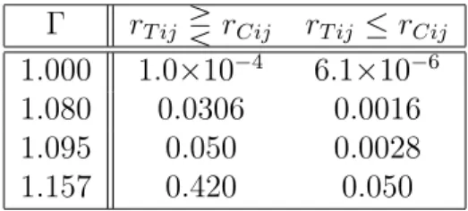
The results of a sensitivity analysis for a test of δ = 0 ⇔ ϕ = 1 with a lower one-sided alternative are shown in Table 2. As one can see, the result is sensitive to unobserved biases under both scenarios, but far more so when we do not make an assumption on the direction of effect. To better understand this, it is useful to think of the corresponding integer programs that result in these worst-case bounds. The optimization problem with the assumption of a nonpositive treatment effect has 2,830 variables associated with it, with variables only corresponding to a choice of vectoru−i
in a given stratum. Without making this assumption, the number of variables grows to 321,860, as we must consider all non-exchangeable allocations of potential outcomes
andall choices for the vector of unmeasured confounders. The difference in problem size impacts not only design sensitivity, but also computation time. The computations for each value ofΓ>1shown took an average of 1.5 seconds under the assumption of non-negativity, but 75 seconds without this assumption. See Appendix F for a discussion of why the assumption of a known direction of effect has such a substantial impact. Considering the sheer size of the problem, this bears testament to the strength of our formulation: for all of the Γ values tested, the continuous relaxation had an integer solution.
6.2
Effect Ratio
Yang et al. (2014) present an observational study comparing the effect of cesarian section versus vaginal delivery on the survival of premature babies of 23-24 weeks gestational age, where Rij = 1 if a baby survives. The analysis used whether or not a baby was
delivered at a hospital with “high” rates of c-section as a potential instrumental variable. We present a sensitivity analysis for these data under combinations of assumptions of
Table 2: Sensitivity analysis for an one-sided test with alternative hypothesis δ < 0⇔ ϕ <
1. Worst case p-values are shown with (rightmost column) and without (middle column)
assuming a known direction of effect.
Γ rT ij RrCij rT ij ≤rCij
1.000 1.0×10⁻⁴ 6.1×10⁻⁶
1.080 0.0306 0.0016
1.095 0.050 0.0028
1.157 0.420 0.050
varying strength. In so doing, we aim to assess the impact of various assumptions on the inference’s perceived sensitivity to unmeasured confounding. 1489 pairs of babies were formed, with a baby in the “high” group being matched to baby in the “low” group who was similar on the basis of all other pre-treatment covariates. Let Zij = 1 if the
baby was delivered at a hospital with a high c-section rate, and letDij = 1if the baby
was delivered by a c-section. As such, the “randomized encouragement” is the type of hospital at which the baby was delivered, and the treatment of interest is the actual method of delivery.
We present inference on the effect ratio under all eight combinations of enforcing and not enforcing a nonnegative direction of effect (DE) :rT ij ≥rCij ∀i, j; monotonicty
(MO):dT ij ≥dCij ∀i, j , and the exclusion restriction (ER):dT ij =dCij ⇒rT ij =rCij
∀i, j. In the context of this example, the effect ratio is the ratio of the increase in survival rate to the increase in rate of c-sections for premature babies of 23-24 weeks gestational age that occurs with being delivered at a hospital with a high rate of c-sections. If we additionally assume that both monotonicity and the exclusion restriction hold, then the effect ratio has the additional interpretation of being the effect of delivering at a hospital with high rates of c-sections among babies who would have been delivered by c-section if and only if they were delivered at a hospital with a high rate of c-sections. Under any combination of assumptions, the estimated effect ratio is λˆ = 0.866. Assuming none of (DE), (MO), (ER), the 95% confidence interval is [0.50; 1.47], and there are 256 decision variables in the optimization problem. Assuming all of (DE), (MO), (ER), the 95% confidence interval shrinks to [0.58; 1], and there are 49 decision variables in the optimization problem.
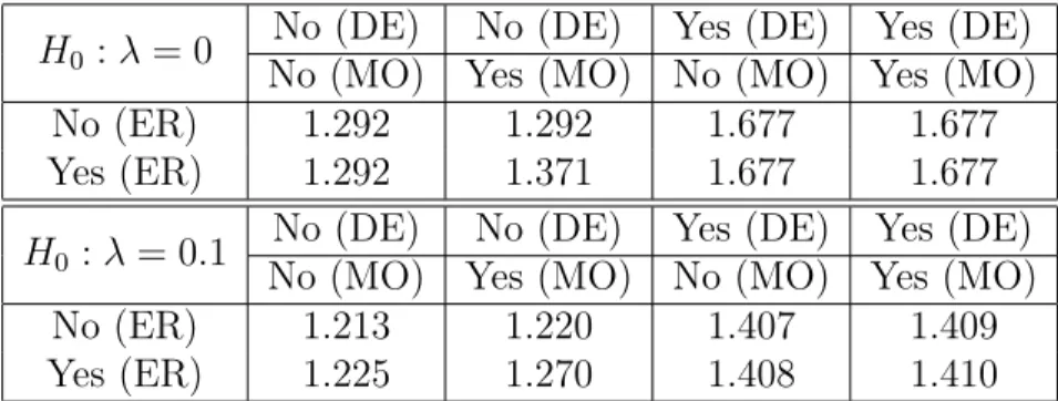
In Table 3, we present the values ofΓrequired to overturn the rejection of the nulls that λ = 0 and λ= 0.1, both with an upper one-sided alternative at α = 0.05. For the null of λ= 0, this test boils down to a test on the average treatment effect, but with a range of restrictions on the potential outcomes. Once a nonnegative direction of effect is imposed (the bottom four cells of the table), the test ofλ= 0 simply becomes a test of Fisher’s sharp null; see Appendix F for further discussion. Because of this, the assumptions of monotonicity and the exclusion restriction cannot impact the sensitivity analysis atλ= 0unless non-negativity is not enforced. Furthermore, without assuming a direction of effect, monotonicity can only affect the performed inference if it is enforced in concert with the exclusion restriction atλ= 0and vice versa. Forλ= 0.1, the test no longer corresponds exclusively to one of Fisher’s sharp null when non-negativity is imposed. We thus see that each assumption impacts the study’s robustness against
Table 3: Minimal value of Γ such that conclusion of the hypothesis test on λ is reversed under eight combinations of assumptions.
H0 :λ= 0
No (DE) No (DE) Yes (DE) Yes (DE)
No (MO) Yes (MO) No (MO) Yes (MO)
No (ER) 1.292 1.292 1.677 1.677
Yes (ER) 1.292 1.371 1.677 1.677
H0 :λ = 0.1
No (DE) No (DE) Yes (DE) Yes (DE)
No (MO) Yes (MO) No (MO) Yes (MO)
No (ER) 1.213 1.220 1.407 1.409
Yes (ER) 1.225 1.270 1.408 1.410
unmeasured confounding to varying degrees. For all combinations of assumptions and each value of Γtested, the corresponding integer quadratic program solved in under 2 seconds.
7
Discussion
Our formulation exploits attributes of the randomization distributions for our proposed test statistics which are unique to inference after matching. While this is sufficient for our purposes, one resulting limitation is that our method will likely not be practicable in observational studies or randomized clinical trials where there either are no strata, or where each stratum contain a large number of both treated and control individu-als; see Rigdon and Hudgens (2015) for a discussion of the difficulties of conducting randomization inference with binary outcomes in these settings. In these settings, the work of Cornfield et al. (1959) presents a method for sensitivity analysis for the risk ratio, and Ding and Vanderweele (2014) extend this approach to the risk difference. Another limitation is that as with any N P-hard endeavor, it is difficult to anticipate ahead of time how long our method will take on a given data set with a given match structure; however, through a host of simulation studies presented both in Section 5.3 and Appendix D we have provided further insight into these matters for practitioners interested in using our methods.
We have framed hypothesis testing and sensitivity analyses for composite null hy-potheses with binary outcomes in matched observational studies as the solutions to integer linear (Γ = 1) and quadratic (Γ>1)programs. An interesting consequence of our formulation is that it readily yields a method for performing a sensitivity analysis for simple null hypotheses under general outcomes without reliance on the asymptoti-cally separable algorithm of Gastwirth et al. (2000); see Appendix G for details and a data example. We have shown that our method can be practicable even with large data sets and large stratum sizes. We have further demonstrated through simulation studies and real data examples that our formulation explicitly avoids issues known to hinder the performance of integer programming algorithms such as looseness of formulation and symmetry. In so doing, we hope to shed further light on the usefulness of integer programming for solving problems in causal inference.
APPENDIX
A
Balance on Observed Covariates in Our
Moti-vating Example
Standardized Differences Before and After Matching
Standardized Differences
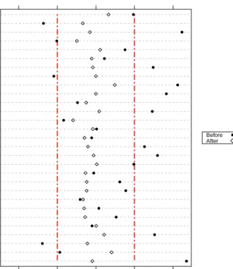
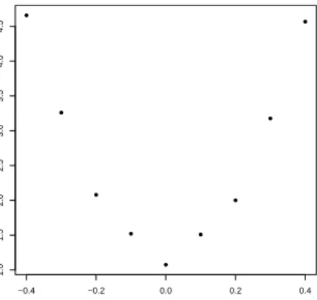
Penn Presby. Med. Center Pennsylvania Hospital Hosp. of Univ. of Penn. Disease Severity Index Marital Status Insurance Category Pneumonia Myocardial Infarction Septic Shock Severe Sepsis Sepsis Tracheostomy Tube Endotracheal Tube Acute Respiratory Failure Acute Dialysis Hypoglycemia Congestive Heart Failure Acute Brain Dysfunction Charlson Comorbidity Index ICU Admission Length of Stay Admission Type: Urgent Any Procedures? Low Sodium Low Hemoglobin Oncology Number of Procedures Num. of Prev. Hospitalizations Age −0.4 −0.2 0.0 0.2 0.4 ● ● ● ● ● ● ● ● ● ● ● ● ● ● ● ● ● ● ● ● ● ● ● ● ● ● ● ● ● Before After ●
Figure 1: Covariate Imbalances Before and After Matching. The dotplot (a Love plot) shows the
absolute standardized differences without matching, and after conducting a matching with a variable number of controls. The vertical dotted line corresponds to a standardized difference threshold of 0.2, which is often regarded as the maximal allowable absoute standardized difference (Rosenbaum, 2010). As one can see, marked imbalances existed between the two populations before matching. All standardized differences were below 0.2 after matching, and most covariates saw substantial improvements in balance through matching.
B
Treatment Effects and Treatment Effects on
the Treated
In determining whether interest should lie in the attributable effect of Rosenbaum (2001, 2002a) rather than the risk difference or risk ratio, one must decide whether the question of interest concerns the treatment effect on the entire study population, or rather only
concerns the effect of the intervention for those individuals who were treated. The attributable effect is itself a treatment effect on the treated, in that it is defined as
A=PI
i=1
Pni
j=1Zij(rT ij−rCij), whereas the risk difference and risk ratio concern the
effects of the treatment for the entire study population. While the group of treated individuals will look the same as the overall study population in a randomized clinical trial, these two groups of individuals can be quite different in observational studies due to self-selection. Thus, these estimands speak to different sets of individuals in the study population.
In the example presented in Section 1.2 on hospital readmission rates, if we define the treatment group as the individuals who went to acute care rehabilitation and as-sign a response of 1 (a “success”) to individuals did not require hospital readmission, the attributable effect then compares the number of individualsassigned an acute
rehabil-itation center who were not rehospitalized to what that number would have been if all
the individuals who went to acute rehabilitation actually used home with home health services for their rehabilitation. If we additionally assume a nonnegative treatment effect, the attributable effect would have an additional interpretation as the number of individuals assigned to an acute rehabilitation center who avoided rehospitalization because of the acute rehabilitation center (i.e., who would have been rehospitalized had they instead utilized home with home health services for their rehabilitation). The risk difference, on the other hand, would compare the proportion of individuals in the
entire study population who would have avoided rehospitalization if all individuals had
been assigned to acute rehabilitation to the proportion avoiding rehospitalization if all individuals utilized home with home health services.
The determination of which target population (the entire study population versus only the individuals who received the treatment) is most relevant often depends on the research question being investigated. Austin (2010) notes that “applied researchers should decide whether the [average treatment effect] or the [average treatment effect on the treated] is of greater utility or interest in their particular research context.” He then provides two examples to illustrate why the estimand of greatest relevance dependence is not uniform across applications. He notes that if one where investigating the effectiveness of an intensive and structured smoking cessation program, the treated individuals alone may be of greater interest as many smokers may not be interested in the program due to its intensive nature. On the other hand, if the program instead involved physicians giving brochures to patients, then the effect on theentire population of smokers (both those receiving and those not receiving the brochure) may be of greater interest as there are minimal barriers to a patient receiving the treatment (the brochure). Heckman and Robb (1985) and Heckman et al. (1997) further argue that the treated units themselves are often of more interest than the overall population if the intervention is narrowly targeted (e.g., if it is such that most controls would never consider undergoing the intervention).
Investigation of the average treatment effect (risk difference) has long been a pur-suit of great interest in randomized experiments (Neyman, 1923), and this interest has carried over to the analysis of observational studies. For example, Imbens (2004) notes that the average treatment effect is the most commonly studied causal estimand in econometric literature. Investigating the attributable effect while also assuming a known direction of effect can remove the need for integer programming in conducting inference and sensitivity analyses (Rosenbaum, 2002a); however, one must be sure that
the attributable effect is the most appropriate estimand for the problem at hand before pursuing inference on it. This determination should not be made solely on the basis of computational complexity. In many cases the risk difference and risk ratio may be more appropriate, and in these instances the methodology presented in this work can facilitate inference and sensitivity analyses.
C
Usage of Risk Differences and Risk Ratios
The risk difference and risk ratio are two measures of the causal effect of an intervention on a binary outcome. A common viewpoint taken in the statistics literature is that the appropriateness of using the risk ratio (also called the relative risk) versus the risk difference depends on the scale of the problem, with certain measures being appropriate for certain inferences. This is discussed in Hernán and Robins (2016) in the following paragraph:
Each effect measure may be used for different purposes. For example, imag-ine a large population in which 3 in a million individuals would develop the outcome if treated, and 1 in a million individuals would develop the out-come if untreated. The causal risk ratio is 3, and the causal risk difference is 0.000002. The causal risk ratio (multiplicative scale) is used to compute how many times treatment, relative to no treatment, increases the disease risk. The causal risk difference (additive scale) is used to compute the abso-lute number of cases of the disease attributable to the treatment. The use of either the multiplicative or additive scale will depend on the goal of the inference. (Hernán and Robins, 2016, pages 7-8)
Of course, the converse can be true: if 85% develop the outcome if treated and 80% develop the outcome if not treated, the risk ratio is then 1.0625 while the risk difference is 0.05. Grieve (2003) provides additional discussion of these two estimands, noting that in deciding which estimand to use one must consider “whether interest is centered on absolute or relative effects, and the extent to which those who are to use them understand them” (Grieve, 2003, page 88).
The summary measure chosen can also affect the extent to which a study’s findings influence future action. Misselbrook and Armstrong (2001) note that when deciding whether or not to take a proposed treatment the percentage of individuals who end up agreeing to take the treatment can vary substantially depending on whether the benefits of a treatment are presented in the form of a risk ratio or a risk difference. Forrow et al. (1992) note that the manner in which information on a causal effect is presented can affect not only how likely patients are to take a recommended treatment, but also how likely a doctor is to prescribe a treatment in the first place.
Poole (2010) states that in epidemiology, it has been treated as a seemingly self-evident truth that “relative effect measures should be used to assess causality and that absolute measures should be used to assess impact.” (Poole, 2010, page 3). An early defense of this stance can be found in the work of Cornfield et al. (1959) on smoking and lung cancer:
Both the absolute and the relative measures serve a purpose. The rela-tive measure is helpful in (1) appraising the possible noncausal nature of an