Algorithms for Nonconvex Optimization
Problems in Machine Learning and Statistics
Zur Erlangung des akademischen Grades eines Doktors der Wirtschaftswissenschaften
Dr. rer. pol.
von der KIT-Fakultät für Wirtschaftswissenschaften des Karlsruher Instituts für Technologie (KIT)
genehmigte DISSERTATION
von
M. Sc. Robert Mohr
Tag der mündlichen Prüfung: 11.03.2020
Referent: Prof. Dr. Oliver Stein
Contents
1 Thesis Overview 1
I
A Trust-Region Method for the Local Solution of
Large-Scale Finite-Sum Problems
3
2 Introduction 5
2.1 Machine Learning and Finite-Sum Minimization . . . 5
2.2 Optimization in Machine Learning . . . 6
2.3 Trust-Region Methods for Finite-Sum Minimization . . . 7
2.4 Overview of our Approach . . . 8
3 Adaptive Sample Size TR Method 11 3.1 The ASTR-Algorithm . . . 11 3.1.1 Outer Iterations . . . 12 3.1.2 Inner Iterations . . . 12 3.1.3 Trust-region step . . . 13 3.2 Theoretical Analysis . . . 14 3.2.1 Assumptions . . . 14 3.2.2 Theoretical Results . . . 16 3.3 Practical Considerations . . . 19
3.3.1 Random Sampling and Sample Size Adjustment . . . . 20
3.3.2 Incorporation of Curvature Information and the Solu-tion of the Trust-Region Subproblems . . . 20
3.3.3 Adjusting the Number of Inner Iterations . . . 21
4 Numerical Experiments 23 4.1 Logistic Regression . . . 24
4.2 Nonlinear Least-Squares . . . 25
4.3 Neural Network Training . . . 27
4.4 Conclusions . . . 28 i
Spline Approximation Problem with Free Knots
31
5 Introduction 33
5.1 Curve Fitting with Splines . . . 33
5.2 The Least-Squares Spline Approximation Problem . . . 34
5.2.1 The Problem with Fixed Knots . . . 35
5.2.2 The Problem with Free Knots . . . 38
5.3 Literature review of existing approaches . . . 39
5.4 Overview of our Approach . . . 40
6 A Combinatorial Formulation 45 6.1 Reformulation as a Set Partitioning Problem . . . 45
6.2 Formulation as a Mixed-Integer Optimization Problem . . . . 46
6.2.1 Feasible Partitions . . . 48
6.2.2 Continuity Restrictions . . . 50
6.2.3 Generalized Epigraph Reformulation . . . 51
6.3 Alternative Error Functions . . . 54
6.3.1 Absolute Error Function . . . 54
6.3.2 Maximum Error Function . . . 56
7 A Branch-and-Bound Algorithm 57 7.1 General Outline of the Branch-and-Bound Algorithm . . . 57
7.2 Branching Strategy . . . 58
7.3 Computation of Lower Bounds . . . 61
7.4 The Branch-and-Bound Algorithm . . . 63
8 Numerical Experiments 65 8.1 Comparison with Existing Approaches . . . 65
8.2 Comparison of MIQCP and B&B Approaches . . . 68
8.2.1 Titanium Heat and Angular Displacement Data Sets . 69 8.2.2 Synthetic Data Sets . . . 70
8.2.3 Computation of Piecewise Polynomials . . . 73
9 Conclusions and Outlook 79 A Results of the Numerical Experiments 87 A.1 Large-Scale Finite-Sum Minimization . . . 87
A.2 Least-Squares Spline Approximation with Free Knots . . . 105
A.3 Least-Squares Polynomial Approximation with Free Knots . . 119
List of Figures
4.1 Logistic regression error of SGD, SVRG, TR and ASTR for all data sets. . . 26 4.2 Further details on the performance of SGD, SVRG, TR and
ASTR on the logistic regression problem with the odd_even data set. . . 27 4.3 Further details on the performance of SGD, SVRG, TR and
ASTR on the logistic regression problem with theHIGGS data set. . . 28 4.4 Nonlinear least-squares error of SGD, SVRG, TR and ASTR
for all data sets. . . 29 4.5 Performance of SGD, SVRG, TR and ASTR on the neural
network training problem with theMNIST data set. . . 30 5.1 Objective function of the least-squares spline approximation
problem with two free knots and the optimal least-squares spline functions. . . 42 5.2 Objective function of the least-squares spline approximation
problem with two free knots. . . 43 5.3 Locally and globally optimal least-squares spline functions with
two knots. . . 44 8.1 Spline functions with three free knots corresponding to the
solutions obtained with the FR, CG, CF and CF+FR methods when applied to the titanium heat data set. . . 67 8.2 Spline functions with five free knots corresponding to the
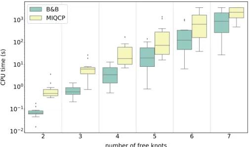
so-lutions obtained with the FR, CG, CF and CF+FR methods when applied to the angular displacement data set. . . 69 8.3 CPU times (in seconds) required by the B&B and MIQCP
approaches in order to compute the optimal spline functions with three free knots for various data set sizes. . . 72
approaches in order to compute the optimal spline functions
for 50 data points and various numbers of free knots. . . 74
8.5 CPU times (in seconds) required by the B&B and MIQCP approaches in order to compute the optimal piecewise polyno-mials with three free knots anf various data set sizes. . . 76
8.6 CPU times required by the B&B and MIQCP approaches in order to compute the optimal piecewise polynomials for 100 data points and various numbers of free knots. . . 78
A.1 Performance of SGD, SVRG, TR and ASTR on the logistic regression problem with data set a9a. . . 89
A.2 . . . on the data set w8a . . . 90
A.3 . . . on the data set odd_even. . . 91
A.4 . . . on the data set ijcnn. . . 92
A.5 . . . on the data set skin. . . 93
A.6 . . . on the data set covertype. . . 94
A.7 . . . on the data set SUSY. . . 95
A.8 . . . on the data set HIGGS. . . 96
A.9 Performance of SGD, SVRG, TR and ASTR on the nonlinear least squares problem with data set a9a. . . 97
A.10 . . . on the data set w8a. . . 98
A.11 . . . on the data set odd_even. . . 99
A.12 . . . on the data set ijcnn. . . 100
A.13 . . . on the data set skin. . . 101
A.14 . . . on the data set covertype. . . 102
A.15 . . . on the data set SUSY. . . 103
A.16 . . . on the data set HIGGS. . . 104
List of Tables
8.1 Least-squares errors of the solutions obtained with the FR, CG, CF and CF+FR methods when applied to the titanium heat data set. . . 66 8.2 Least-squares errors of the solutions obtained with the FR,
CG, CF and CF+FR methods when applied to the angular displacement data set. . . 68 8.3 CPU times and least-squares errors of the solutions obtained
with the B&B and MIQCP approaches for the titanium heat data set. . . 70 8.4 CPU times and least-squares errors of the solutions obtained
with the B&B and MIQCP approaches for the angular dis-placement data set. . . 70 8.5 Combinations of data set sizes and number of free knots when
generating instances of the spline approximation problem. . . 71 8.6 Percentage of solved instances and average CPU times
re-quired by the B&B and MIQCP approaches to compute the optimal spline functions with three free knots for various data set sizes. . . 73 8.7 Percentage of solved instances and average CPU times
re-quired by the B&B and MIQCP approaches to compute the optimal spline functions for 50 data points and various num-bers of free knots. . . 75 8.8 Combinations of data set sizes and number of free knots when
generating instances of the piecewise polynomial approxima-tion problem. . . 75 8.9 Percentage of solved instances and average CPU times (in
sec-onds) required by the B&B and MIQCP approaches to com-pute the optimal piecewise polynomials with three free knots and various data set sizes. . . 77
quired by the B&B and MIQCP approaches to compute opti-mal piecewise polynomials for 100 data points various numbers
of free knots. . . 78
A.1 Data sets used in the numerical experiments on large-scale finite-sum minimization. . . 88
A.2 An overview of the functions used to generate the synthetic data sets used in the numerical experiments on least-squares spline and piecewise polynomial approximation problems. . . . 106
A.3 Results of the B&B and MIQCP approaches for the computa-tion of least-squares splines for the coslin data sets. . . 107
A.4 . . . for the cube data sets. . . 108
A.5 . . . for the arctan data sets. . . 109
A.6 . . . for the rational data sets. . . 110
A.7 . . . for the Inhom1 data sets. . . 111
A.8 . . . for the Inhom2 data sets. . . 112
A.9 . . . for the Inhom3 data sets. . . 113
A.10 . . . for the logit data sets. . . 114
A.11 . . . for the bump data sets. . . 115
A.12 . . . for the sine3 data sets. . . 116
A.13 . . . for the sine6 data sets. . . 117
A.14 . . . for the SpaHet3 data sets. . . 118
A.15 Results of the B&B and MIQCP approaches for the computa-tion of piecewise polynomials for the coslin data sets. . . 120
A.16 . . . for the cube data sets. . . 121
A.17 . . . for the arctan data sets. . . 122
A.18 . . . for the rational data sets . . . 123
A.19 . . . for the Inhom1 data sets. . . 124
A.20 . . . for the Inhom2 data sets. . . 125
A.21 . . . for the logit data sets. . . 126
A.22 . . . for the bump data sets. . . 127
A.23 . . . for the sine3 data sets. . . 128
A.24 . . . for the sine6 data sets. . . 129
A.25 . . . for the SpaHet3 data sets . . . 130
Abbreviations
Part IARC Adaptive regularization method with cubics ASTR Adaptive subset trust-region method
SGD Stochastic gradient descent method
SVRG Stochastic variance reduced gradient method TR Trust-region method
Part II
B&B Branch-and-bound algorithm
CF Combinatorial formulation of the continuous least-squares spline approximation problem with free knots
CF Combinatorial formulation
CF+FR Fletcher-Reeves nonlinear conjugate gradient method initialized with the solution to the combinatorial formulation
CG Continuous genetic algorithm
FR Fletcher-Reeves nonlinear conjugate gradient method initialized with the equidistant knot placement
LP Linear optimization problem
MILP Mixed-integer linear optimization problem
MIQCP Mixed-integer quadratically constrained optimization problem
Notation
General Mathematical Notation
N Natural numbers 1,2,3. . .
Rn Real coordinate space ofn dimensions
[a, b] Line segment between the vectorsa, b∈Rn
Rm×n Space of real matrices with m rows and n columns Sn Space of real symmetric matrices of dimensionn
hx, yi Canonical inner producthx, yi=x|y in
Rn
kxk2 Euclidean norm of a vectorx∈Rn
kAk2 Spectral norm of a matrix A∈Rm×n
|S| Cardinality of the set S S\T Set difference ofS and T C2(
Rn,R) Space of twice continuously differentiable functions with
domainRn and codomain
R
∇f Gradient of the differentiable function f :Rn →R
D2f Hessian of the twice differentiable functionf :
Rn→R
Part I
n Number of data points
m Dimension of the decision variable
F Objective function of the finite-sum problem
fi Functions summed up in objective functionF
S Sample of data points
Sν,k Sample of data points in iteration ν, k
SHν,k Sample of data points used for the curvature approximation in iterationν, k
sν Sample size in iterationν FS Sampled objective function
Fν,k Shorthand forF Sν,k
xν Outer iterate in iteration ν xν,k Inner iterate in iterationν, k
qν,k(·) Quadratic model function of Fν,k atxν
gν,k Shorthand for∇Fν,k(xν,k) ix
A Matrix containing curvature information of F ρν,k Ratio of actual to predicted improvement
δν Trust-region radius
Rν Number of inner iterations
b
R Upper limit on the number of inner iterations
θ Parameter controlling the sample size adjustment
aν Progress on the objective function F in iteration
bν Average progress during the inner iterations on FS
dν,k Trust-region step in iteration ν, k Part II
n Number of data points
k Number of free knots
β Vector of coefficients of a spline function
ξ Knots of a spline function
s(·, β, ξ) Spline function with parameter vector β and knot vector ξ p(·, β) Cubic polynomial with parameter vector β
p0(·, β) First derivative of p(·, β)
p00(·, β) Second derivative of p(·, β)
Ij Set of indices of data points assigned to the jth polynomial
I Set of unassigned indices
Xj Vandermonde matrix corresponding to the data points with indices in Ij
zij Binary variable that is one if data point i is assigned to the
jth polynomial
Λj jth restriction set Λj ⊆ {1, ..., n} max(Λj) Largest element in Λj
min(Λj) Smallest element in Λj
Chapter 1
Thesis Overview
Mathematical optimization is one of the pillars of machine learning and mod-ern statistics. Optimization algorithms are used to compute parameters of model functions such that available data is approximated optimally with re-spect to some error criterion. The numerical efficiency of these optimization algorithms is of key importance concerning the overall effectiveness of many of the techniques used to tackle problems in data science.
The purpose of this thesis is the design of algorithms that can be used to determine optimal solutions to nonconvex data approximation problems. If such a problem is large-scale, i.e. the decision variable is high dimensional and/or the number of data points is large, the computation of globally op-timal solutions is usually not a realistic goal. Instead, local optimization algorithms can be used to efficiently approximate locally optimal solutions. And despite the fact that in the nonconvex case locally optimal solutions can be far from globally optimal, there are relevant large-scale problem classes in machine learning, e.g., the training of neural networks, for which local opti-mization algorithms are very effective empirically and therefore very popular. Naturally, there also exist nonconvex data approximation problems where lo-cal optimization algorithms get stuck in suboptimal lolo-cal solutions if they are not initialized in a sufficiently small neighborhood of the global solution. Here it is necessary to develop algorithms that compute solutions close to the globally optimal solution, such that theses solutions can be used as starting points in local optimization algorithms.
In Part I of this thesis, we consider a very general class of nonconvex and large-scale data approximation problems and devise an algorithm that efficiently computes locally optimal solutions to these problems. After the introduction and literature review in Chapter 2, we present our algorithm in Chapter 3. In contrast to most algorithms proposed in the machine learning literature, our algorithm is a second-order method, i.e., it incorporates
vature information of the objective function in the computation of the search direction. As a type of trust-region Newton-CG method, the algorithm can make use of directions of negative curvature to escape saddle points, which otherwise might slow down the optimization process when solving nonconvex problems. In Chapter 4 we present results of numerical experiments on con-vex and nonconcon-vex problems which support our claim that our algorithm has significant advantages compared to current state-of-the-art methods. Part I of this thesis is based on the preprint Mohr and Stein (2019).
In Part II we consider a specific nonconvex data approximation prob-lem which is known to possess a large number of locally minimal points far from the globally optimal solution, namely the univariate least-squares spline approximation problem with free knots. In Chapter 5 we introduce the opti-mization problem and review existing approaches for its solution. Moreover, we show that local optimization algorithms, like the one presented in the first part of this thesis, should not be expected to yield satisfactory solutions for this problem if the initial point is not chosen sufficiently close to a globally op-timal solution. However, since in typical applications, neither the dimension of the decision variable nor the number of data points is particularly large, it is possible to make use of the specific problem structure in order to de-vise algorithmic approaches to approximate the globally optimal solution of problem instances of relevant sizes. In Chapter 6 we propose to approximate the continuous original problem with a combinatorial optimization problem and, as a first algorithmic approach for the solution of the latter, we present a convex mixed-integer formulation that can be solved with commercial op-timization solvers. As an alternative algorithmic approach, we propose a branch-and-bound method in Chapter 7, which is tailored specifically to the combinatorial problem formulated in the previous chapter. In Chapter 8 we present numerical experiments on real and synthetic data which show that the combinatorial approach to the least-squares spline approximation prob-lem with free knots makes it possible to compute high-quality solutions to problems of realistic sizes within reasonable computing times. Part II of this thesis is based on joint work with Dr. Maximilian Coblenz and Dr. Peter Kirst.
Parts I and II of this thesis are concerned with the same basic problem of data approximation. However, the optimization methods that are proposed range from randomized local methods for continuous problems to determin-istic global methods for discrete problems. This shows that when dealing with the difficult problem of nonconvexity in data science applications, it is important to make use of diverse tools from mathematical optimization in order to obtain high-quality solutions.
Part I
A Trust-Region Method for the
Local Solution of Large-Scale
Finite-Sum Problems
Chapter 2
Introduction
In this chapter, we first describe how the finite-sum minimization problem arises naturally in machine learning applications. Then we review existing algorithmic approaches to the large-scale finite sum minimization problem, before giving an overview of our approach.
2.1
Machine Learning and Finite-Sum
Mini-mization
There exists a variety of applications from statistics and machine learning that require the minimization of an objective function that is the sum of a large number of convex or nonconvex functions. Well known examples are logistic regression problems, the training of neural networks and nonlin-ear least-squares problems. In these applications, the number of functions summed up in the objective function typically corresponds to the number of data points considered.
A typical task in supervised machine learning is prediction. Suppose we are given a data set (xi, yi)∈Rr×
Rz,i= 1, . . . , n, and a family of prediction
functionsh(·, w) :Rr →
Rz parametrized with a vector w∈Rm. The goal is
to find a parameter ¯wsuch that the probability is high that if (¯x,y¯) is a new and so far unseen data point, we have thath(¯x,w¯)≈y¯. This is referred to as generalization in the machine learning literature. However, since we have no information apart from the given data set, the most natural way to approach this task is to compute the global minimizer of the finite-sum problem
min w∈Rm n X i=1 `(h(xi, w), yi), (2.1) 5
where ` : Rz ×
Rz → R is an error function that quantifies the discrepancy
betweenh(xi, w) and the actual valueyi corresponding to xi. In the machine learning literature, ` is typically called a loss function and problem (2.1) is referred to as the empirical risk minimization problem.
2.2
Optimization Algorithms in Large-Scale
Machine Learning
Successful algorithms from classical nonlinear optimization, such as quasi-Newton, nonlinear conjugate-gradient and trust-region methods, usually re-quire the computation of the gradient and (approximate) Hessian of the objective function in every iteration. If the number of data points is very large, these computations are expensive and prohibit fast progress in the early stages of the optimization process.
Popular methods therefore use single data points or samples of data points (so-called mini-batches) in order to obtain approximate information about the objective function. Arguably the most well-known and successful algo-rithms in this area are the stochastic gradient descent method, which was first proposed by Robbins and Monro (1951), and its variance-reduced vari-ants (e.g., Schmidt et al. 2017, Defazio et al. 2014, Johnson and Zhang 2013), in which single data points or mini-batches are used in order to approximate the gradient of the objective function. We refer the interested reader to the excellent surveys by Bottou et al. (2018) and Curtis and Scheinberg (2017) for details concerning these methods. However, these methods have two ma-jor drawbacks. Firstly, extensive experimentation is needed for every new problem and data set in order to find hyper-parameters (e.g., the step-size) that lead to a good performance of these methods. Secondly, since only first-order information is employed, their ability to make progress in the presence of saddle points or to deal with ill-conditioned problems is limited.
In the last few years there has been growing interest in algorithms that speed up the minimization of large-scale finite-sum problems by incorporating approximate second-order information via sampling. In particular, stochas-tic Newton, Gauss-Newton and (limited-memory) BFGS methods were de-veloped (e.g., Byrd et al. 2011, Roosta-Khorasani and Mahoney 2019, Bol-lapragada et al. 2018b, Martens 2010, Martens and Sutskever 2011, Schrau-dolph et al. 2007, Bordes et al. 2009, Sohl-Dickstein et al. 2014, Mokhtari et al. 2015, Byrd et al. 2016, Berahas et al. 2016, Curtis 2016, Gower et al. 2016, Zhou et al. 2017, Bollapragada et al. 2018c, Berahas and Takáč 2019). However, despite promising theoretical and empirical results, most of the
2.3. TRUST-REGION METHODS FOR FINITE-SUM MINIMIZATION7 proposed methods still depend on extensive hyper-parameter tuning for each new problem and data set. Moreover, all of these methods work with positive definite curvature approximations and experience numerical instability when these matrices become close to singular. However, in the context of noncon-vex optimization, it was demonstrated by Curtis and Robinson (2019) that incorporating directions of negative curvature can be beneficial and, accord-ing to Dauphin et al. (2014), they might help to escape saddle points more quickly.
In this thesis, we propose a trust-region method that can be applied to large-scale nonconvex finite sum minimization. The reason why we propose a trust-region method is that it is very flexible with respect to the type of approximate curvature information that can be used, and can exploit directions of negative curvature. In the next section we discuss the existing literature on trust-region methods for the finite-sum minimization problem.
2.3
Trust-Region Methods for Finite-Sum
Min-imization
Along with nonlinear conjugate gradient and quasi-Newton methods, trust-region algorithms belong to the most reliable and efficient algorithms for the local minimization of general nonlinear functions. Theoretical results concerning global convergence properties of classical trust-region methods, as well as practical considerations, can be found in the books by Conn et al. (2000) and Nocedal and Wright (2006) and the survey paper by Yuan (2015). From a practical point of view, trust-region algorithms for the finite-sum minimization problem proposed so far can be broadly classified into three groups, depending on how sampling is used in order to obtain approximate information about the objective function. Members of the first group eval-uate the objective function and its gradient exactly in each iteration, while using a sample of the data points to determine approximate curvature infor-mation (e.g., Xu et al. 2019, 2017). In addition to approximating curvature information, methods that belong to the second group also approximate the gradient based on a (possibly different) sample, while still evaluating the ob-jective function exactly in every iteration (e.g., Gratton 2017, Yao et al. 2018, Erway et al. 2019). The last group contains methods that, at least in the early stages of the optimization process, only work with inexact information about the objective function based on samples, i.e., the objective function is evaluated inexactly as well (e.g., Chen et al. 2018, Bellavia et al. 2018, Blanchet et al. 2019).
The main idea underlying methods from the first group is that the most expensive step in each iteration of a trust-region method is the (approximate) solution of the trust-region subproblem, at least if nontrivial curvature ap-proximations are employed. This cost can be greatly reduced if the curvature information is approximated based on a small sample of the data points. The global convergence to first order critical points is covered by results on stan-dard trust-region methods. However, since the objective function and its gradient are evaluated exactly in each iteration, the behavior of these meth-ods is more similar to deterministic than to randomized methmeth-ods.
This drawback also applies to the methods of the second group. In typical finite-sum problems from machine learning and statistics, the evaluation of the objective function is about half as expensive as the computation of the gradient. Therefore, although methods that approximate the gradient can be more efficient than methods that use the exact gradient, the progress of these methods will be slow in the early stages of the optimization process as long as the objective function is evaluated in every iteration.
In contrast, methods from the last group can achieve very low per itera-tion costs if the samples used for the approximaitera-tions are sufficiently small. However, in order to obtain a convergent method, the objective function and its gradient have to be approximated with increasing accuracy. In the context of the finite-sum minimization, this necessitates increasing the cor-responding sample size during the optimization process, which is referred to as dynamic/adaptive sampling or progressive batching. This technique leads to hybrid deterministic-stochastic methods, i.e., methods that start off as randomized methods and eventually turn into deterministic methods.
In these methods, the sample size can either be increased at a preset rate or adaptively according to information obtained during the optimiza-tion process. Promising theoretical and empirical results were obtained for the stochastic gradient descent and the stochastic L-BFGS methods (e.g., Friedlander and Schmidt 2012, Byrd et al. 2012, De et al. 2017, Bollapra-gada et al. 2018a,b,c). In the context of trust-region methods, adaptive rules for adjusting the sample size so far either depend on unknown quantities or require experimentation by the user in order to obtain good performance.
2.4
Overview of our Approach
We propose a trust-region method for finite-sum minimization with an adap-tive sample size adjustment technique, which is practical in the sense that it leads to a globally convergent method that shows strong performance empiri-cally without the need for experimentation by the user. During the
optimiza-2.4. OVERVIEW OF OUR APPROACH 9 tion process, the size of the samples is adaptively increased (or decreased) depending on the progress made on the objective function. We prove that after a finite number iterations the sample includes all points from the data set and the method becomes a full-batch trust-region method. Numerical experiments on convex and nonconvex problems support our claim that our algorithm has significant advantages compared to stochastic gradient descent and its variance-reduced versions.
We note that the technique we propose for sample size adjustment could also be used in conjunction with the adaptive regularization method with cubics (ARC) proposed by Cartis et al. (2011a) and Cartis et al. (2011b). The ARC method is an adaptive version of the cubic regularization method first introduced by Griewank (1981). It was shown by Nesterov and Polyak (2006) and Cartis et al. (2011b) that cubic regularization methods and their adaptive variants are, from a worst-case complexity point of view, superior to classical trust-region methods. This fact lead to increased research interest in stochastic variants of these methods (e.g., Kohler and Lucchi 2017, Xu et al. 2017, Cartis and Scheinberg 2018). However, we chose to propose a trust-region method since it was observed in Xu et al. (2017) that they tend to show stronger empirical performance than ARC methods.
Chapter 3
An Adaptive Sample Size
Trust-Region Method
In the first section of this chapter, we present our trust-region method for the finite-sum minimization problem. Then we provide a theoretical analysis which shows that our adaptive sample size adjustment technique eventually increases the sample size to include all data points, which implies global convergence. In the final section we provide some guidance concerning the practical implementation of the method.
3.1
The ASTR-Algorithm
We call our method AdaptiveSample Size Trust-Region method, or ASTR for short. It is specifically designed to solve the finite-sum minimization problem min x∈Rm F(x) := 1 n n X i=1 fi(x),
wheren, m∈Nandfi ∈C2(Rm,R) for alli= 1, . . . , n. The method consists of outer and inner iterations, shown in Algorithm 3.1 and 3.2, respectively. In every inner iteration, a sample S ⊆ {1, . . . , n} is chosen and Algorithm 3.3 is used to compute a trust-region step for the function
FS := 1 |S| X i∈S fi.
After a certain number of inner iterations of Algorithm 3.2, a candidate for the next outer iterate is returned to Algorithm 3.1. There, the candidate is either accepted or rejected and the sample size is adjusted. We now describe the three algorithms in detail.
3.1.1
Outer Iterations
In iteration ν of Algorithm 3.1, Algorithm 3.2 is called with the current iteratexν, sample size sν, initial trust-region radius δν and number of inner iterationsRν as input arguments. It returns to Algorithm 3.1 a candidate for the next iterate xb
ν and a prediction bν of the improvement in the objective function value ifxb
ν is accepted. Moreover, a value δν+1 is returned, which is passed as the initial trust-region radius to Algorithm 3.2 in the next iteration of Algorithm 3.1.
The candidatexb
ν is accepted ifaν, the improvement in the objective func-tion value, is nonnegative. Note that the computafunc-tion of aν is an expensive operation if n is large, sinceF needs to be evaluated at xb
ν. The new sample sizesν+1 is chosen depending on the size of the ratioτν of actual to predicted improvement. A small value ofτν indicates that the sampled functions used in the inner iterations do not approximateF accurately enough and that the sample size should therefore be increased. A large value of τν, however, is an indicator that faster progress in the inner iterations might be possible if the sample size is decreased.
Note that every time the sample size is increased/decreased in the outer iteration, the inner iterations get more computationally expensive/cheap and the number of inner iterations should therefore also be decreased/increased. In Section 3.3 we explain how to update the sample size and the number of inner iterations in order to obtain a method with strong empirical perfor-mance.
3.1.2
Inner Iterations
In iteration k of Algorithm 3.2, a sample Sν,k of size sν is chosen. For notational convenience, we define Fν,k := F
Sν,k and gν,k := ∇Fν,k(xν,k). If
the gradientgν,k does not satisfykgν,kk
2 ≥ε, whereεis a preset threshold, no step is taken and a new sample is selected in the next iteration. Otherwise, a trust-region step dν,k is computed and the initial trust-region radius δν,k+1 for the next iteration is determined with Algorithm 3.3.
AfterR iterations, the last inner iteratexν,R and the current trust-region radiusδν,R are returned to Algorithm 3.1. Additionally, the average improve-ment on the sampled functions during the inner iterations
bν := 1 R R−1 X k=0 bν,k = 1 R R−1 X k=0 Fν,k(xν,k)−Fν,k(xν,k+1)
is returned to Algorithm 3.1 as a prediction for the improvement on the objective function F if xν,R is accepted as the next outer iterate.
3.1. THE ASTR-ALGORITHM 13 Algorithm 3.1 ASTR - Outer Iterations
1: Input: Initial point x0 ∈
Rm, parameters s0,Rb ∈N and δ0, θ >0;
2: for ν = 0,1, . . . do
3: Select the number of inner iterations Rν ∈ {1, . . . ,Rb};
4: Computexb
ν,bν and δν+1 via Algorithm 3.2 with inputsxν, sν, δν, Rν; 5: if sν < n then 6: Set aν =F(xν)−F(xb ν); 7: if aν ≥0 then setxν+1 = b xν elseset xν+1 =xν; 8: if bν >0then setτν =aν/bν else setτν = 0; 9: if τν < θ then 10: Select sν+1 ∈ {sν + 1, . . . , n}; 11: else 12: Select sν+1 ∈ {1, . . . , sν}; 13: end if 14: else 15: Set xν+1 =xb ν and sν+1 =n; 16: end if 17: end for
3.1.3
Trust-region step
In iterationrof Algorithm 3 an (approximate) solutiondrto the trust-region subproblem
min d∈Rm q
ν,k(d) s.t. kdk
2 ≤∆r, (3.1)
is computed, where qν,k is a (quadratic) model of Fν,k atxν,k defined as
qν,k(d) := Fν,k(xν,k) +hgν,k, di+ 1 2d
|Aν,kd,
and ∆r is the current trust-region radius. The matrix Aν,k ∈Sm can be used to include curvature information in the model. However, it is also possible to only use first-order information by settingAν,k = 0.
An (approximate) solution dr to problem (3.1) is accepted if the ratio
ρν,k(dr) := F
ν,k(xν,k+dr)−Fν,k(xν,k)
qν,k(0)−qν,k(dr) (3.2) of the actual improvement on Fν,k to the improvement predicted by the quadratic model is above a certain threshold η1. The intuition behind this is that if the ratio ρν,k(dr) is above this threshold, this is an indication that
Algorithm 3.2 ASTR - Inner Iterations
1: Input: xν, δν, sν and Rν from Algorithm 3.1 and parameter ε >0; 2: Set xν,0 =xν, δν,0 =δν and R =Rν;
3: for k = 0,1, . . . , R−1 do
4: Choose a sample Sν,k ⊆ {1, . . . , n} of size sν; 5: if kgν,kk2 ≥ε then
6: Compute dν,k, δν,k+1 via Algorithm 3.3 with inputs xν,k,gν,k, δν,k; 7: Set xν,k+1 =xν,k+dν,k; 8: Set bν,k =Fν,k(xν,k)−Fν,k(xν,k+1); 9: else 10: Set xν,k+1 =xν,k, bν,k = 0 andδν,k+1 =δν,k; 11: end if 12: end for 13: Output: xb ν =xν,R, bν = 1 R R−1 X k=0 bν,k,δν+1 =δν,R;
the modelqν,k is a good approximation of Fν,k on the feasible set of problem (3.1) (the so called “trust-region”). As long as the ratio (3.2) is smaller then
η1, the trust-region radius is decreased and a new (approximate) solution of the trust-region subproblem is computed. Since we use the exact gradient of Fν,k in our model qν,k, it is always possible to find an acceptable (ap-proximate) solution to the trust-region subproblem if the trust-region radius is sufficiently small (see Theorem 3.2.5). Note that if the ratio (3.2) is not only larger than η1 but also larger than η2, then the trust-region radius is increased such that larger steps might be taken in the next inner iteration.
3.2
Theoretical Analysis
In this section we prove that after a finite number of iterations, the sample size sν reaches n and the ASTR method becomes a full-batch trust-region method.
3.2.1
Assumptions
Assumption 3.2.1 The function F is bounded below on Rm, i.e., there ex-ists a constant κ1 ∈R such that F(x)≥κ1 for all x∈Rm.
Assumption 3.2.2 The functions fi, i = 1, . . . , n, are twice continuously differentiable and their gradients ∇fi are Lipschitz continuous.
3.2. THEORETICAL ANALYSIS 15 Algorithm 3.3 Trust-region step
1: Input: xν,k, gν,k and δν,k from Algorithm 3.2 and parameters η
1, η2 ∈ (0,1) and 0 < γ1 <1< γ2;
2: Set r=−1, ∆0 =δν,k;
3: repeat 4: r ←r+ 1;
5: Compute an (approximate) solution dr of problem min d∈Rm qν,k(d) s.t. kdk2 ≤∆r; 6: Compute ρν,k(dr) := F ν,k(xν,k+dr)−Fν,k(xν,k) qν,k(0)−qν,k(dr) ; 7: Set ∆r+1 =γ1kdrk2; 8: until ρν,k(dr)< η 1 9: if ρν,k(dr)≥η
2 and kdrk2 = ∆r then set ∆+=γ2∆r else set ∆+ = ∆r; 10: Output: dν,k =dr and δν,k+1 = ∆+;
Note that Assumption 3.2.2 implies that the Hessians D2f
i(x) are uni-formly bounded inx for all i. From the triangular inequality it immediately follows that the Hessian of the functionFS is uniformly bounded inx andS, i.e., there exists a constant κ2 >0 such that the inequality
kD2FS(x)k2 ≤κ2 (3.3)
holds for any S ⊆ {1, . . . , n} and x∈Rm.
Assumption 3.2.3 There exists a constant κ3 >0 such that for all ν, k we
have that kAν,kk2 ≤κ3.
Assumption 3.2.3 is trivially satisfied if Aν,k = 0 for allν, k. Due to (3.3) we know that Assumption 3.2.3 is also satisfied if we set Aν,k =D2FS(x) for any S and x.
Assumption 3.2.4 There exists a constant κ4 ∈ (0,1) such that for all
ν, k, r we have that qν,k(0)−qν,k(dr)≥κ4kgν,kk2min( kgν,kk 2 1 +kAν,kk 2 ,∆r).
If dr is a sufficiently accurate approximation of the exact solution of the trust-region subproblem, Assumption 3.2.4 is satisfied. Moreover, there exists
a variety of methods for the inexact solution of the trust-region subproblem such that Assumption 3.2.4 is satisfied, e.g., the truncated conjugate gradient (CG) method by Toint (1981) and Steihaug (1983) or the truncated Lanczos method by Gould et al. (1999).
3.2.2
Theoretical Results
The first two theorems presented in this section are modifications of well known results in the literature on trust-region methods, see, e.g., Theorems 6.4.2 and 6.4.3 in Conn et al. (2000). We include the modified proofs of these two theorems for completeness.
Theorem 3.2.5 Suppose A3.2.2, A3.2.3 and A3.2.4 hold. Then there exists a constant κ5 > 0 such that for all ν, k and r the inequality kdrk2 ≤ κ5
implies that ρν,k(dr)≥η1 holds.
Proof. Define the constant
κ5 :=
(1−η1)κ4ε 1 +κ2+κ3
and assume that kdrk2 ≤κ5 holds. From the definition of ρν,k(dr) it follows that 1−ρν,k(dr) = 1− F ν,k(xν,k)−Fν,k(xν,k +d) qν,k(0)−qν,k(dr) = F ν,k(xν,k +d)−qν,k(dr) qν,k(0)−qν,k(dr) , (3.4) where we used that qν,k(0) = Fν,k(xν,k). From Assumption 3.2.4 we know that qν,k(0)−qν,k(dr)≥κ4kgν,kk2min( kgν,kk 2 1 +kAν,kk 2 ,∆r),
where ∆r denotes the trust-region radius in the subproblem that was used to compute the trust-region step dr. With ∆
r ≥ kdrk2, kgν,kk2 ≥ ε and Assumption 3.2.3 we obtain qν,k(0)−qν,k(dr)≥κ4εmin( ε 1 +κ3 ,kdrk2).
Moreover, due toη1, κ4 ∈(0,1) and κ2 ≥0 we know thatkdrk2 ≤κ5 implies
kdrk
2 ≤ 1+εκ3. Thus, we have
3.2. THEORETICAL ANALYSIS 17 This inequality together with (3.4) yields
1−ρν,k(dr)≤ F
ν,k(xν,k+dr)−qν,k(dr)
κ4εkdrk2
.
Now, it follows from Taylor’s theorem that for someλin the line segment [xν,k, xν,k +d] it holds that
Fν,k(xν,k +dr) = Fν,k(xν,k) +hgν,k, dri+ 1 2(d
r)|D2Fν,k(λ)dr
and together with Assumptions 3.2.2 and 3.2.3 we obtain
Fν,k(xν,k+dr)−qν,k(dr) = 1 2(d r)|D2Fν,k(λ)dr− 1 2(d r)|Aν,kdr ≤ 1 2 kD2Fν,k(λ)k2+kAν,kk2 kdrk2 2 ≤(κ2+κ3)kdrk22. Thus, we have that
1−ρν,k(dr)≤ (κ2+κ3) κ4ε kdrk2 ≤ (κ2+κ3) κ4ε κ5 = (κ2+κ3) κ4ε (1−η1)κ4ε 1 +κ2+κ3 = (κ2+κ3) 1 +κ2+κ3 (1−η1)≤1−η1, and therefore ρν,k(dr)≥η1.
The previous theorem guarantees that Algorithm 3.3 terminates after a finite number of steps. Moreover, it is instrumental in proving the following result.
Theorem 3.2.6 Suppose A3.2.2, A3.2.3 and A3.2.4 hold. Then there exists a constant κ6 >0 such that δν,k ≥κ6 holds for all ν, k.
Proof. Define the constant
κ6 := min(
γ1(1−η1)κ4ε 1 +κ2+κ3
, δ0,0).
Assume, for the purpose of deriving a contradiction, that (ν, k) is the first iteration such that δν,k < κ6. Since κ6 ≤ δ0,0 we have (ν, k) 6= (0,0). Moreover, due to δν−1,R = δν,0 we have k ≥ 1. The value δν,k is calculated via Algorithm 3.3 with ∆0 = δν,k−1 as the initial trust-region. Since (ν, k) is the first iteration such that δν,k < κ6, we know that ∆0 = δν,k−1 ≥ κ6. Since δν,k = ∆
exist a smallest index j ∈ {1, . . . , r} such that ∆j < κ6. Clearly, if j is the first iteration such that ∆j < κ6 holds, it must hold that ρν,k(dj−1) < η1. Consequently, we have that
∆j =γ1kdj−1k2 and thus kdj−1k2 = ∆j γ1 ≤ κ6 γ1 ≤ (1−η1)κ4ε 1 +κ2+κ3 =κ5,
withκ5 as defined in the proof of Theorem 3.2.5. From Theorem 3.2.5 it now follows that the inequality ρν,k(dj−1) ≥ η1 holds, which is a contradiction since we already argued thatρν,k(dj−1)< η
1.
Theorem 3.2.7 Suppose A3.2.2, A3.2.3 and A3.2.4 hold. Then there exists a constant κ7 >0 such that for all ν either bν = 0 or bν ≥κ7 holds.
Proof. For any k, if kgν,kk2 < ε, then bν,k = 0. On the other hand, if
kgν,kk2 ≥ ε, then Theorem 3.2.5 guarantees that Algorithm 3.3 terminates with a trust-region step dν,k that satisfies ρν,k(dν,k) ≥ η
1. Thus, we obtain from (3.2) and Assumption 3.2.4 that
bν,k =Fν,k(xν,k)−Fν,k(xν,k+1)≥η1 qν,k(0)−qν,k(dν,k) ≥η1κ4kgν,kk2min( kgν,kk 2 1 +kAν,kk 2 ,∆ν,k),
where ∆ν,k denotes the trust-region radius in the subproblem that was used to compute the trust-region stepdν,k. From Theorem 3.2.6 it follows that
∆ν,k ≥ δ
ν,k
γ2
≥ κ6
γ2 and from Assumption 3.2.3 we know that
kgν,kk 2 1 +kAν,kk 2 ≥ kg ν,kk 2 1 +κ3 .
We therefore have that
bν,k ≥η1κ4εmin( ε 1 +κ3 ,κ6 γ2 ). Thus, sincebν = 1 Rν Rν−1 X k=0
bν,k, we either havebν = 0 orbν ≥κ7, with
κ7 := η1κ4ε b R min( ε 1 +κ3 ,κ6 γ2 )>0.
3.3. PRACTICAL CONSIDERATIONS 19 Concerning the previous theorem, we note that bν = 0 can only occur if
kgν,kk2 < εfor all inner iterations.
Theorem 3.2.8 Suppose A3.2.1, A3.2.2, A3.2.3 and A3.2.4 hold. Then there exists a ν0 ∈N such that sν =n holds for all ν ≥ν0.
Proof. We show that there exists a ν0 ∈N such that sν0 =n since this implies the assertion in the theorem. Assume, for the purpose of deriving a contradiction, that sν < n for all ν ∈
N. Since τν < θ implies sν+1 > sν,
there does not exist a ¯ν ∈ N such that τν < θ for all ν > ν¯. Thus, there exists a subsequence (xν(j)) with τν(j) ≥ θ for all j ∈ N. This implies that
bν(j) > 0 for all j ∈
N. From Theorem 3.2.7 we now obtain that bν(j) > κ7 and therefore
F(xν(j))−F(xb
ν(j)) =aν(j) ≥θbν(j)≥θκ 7
for all j ∈N. Since the sequence (F(xν)) is monotonically nonincreasing we obtain for all i∈N
F(x0)−F(xν(i)+1) = ν(i) X ν=0 (F(xν)−F(xν+1))≥ i X j=0 (F(xν(j))−F(xν(j)+1)) = i X j=0 (F(xν(j))−F(xb ν(j)))≥( i+ 1)θκ7, and therefore F(x0)−F(xν(i)+1)i→∞→ +∞, in contradiction to Assumption 3.2.1.
Theorem 3.2.8 ensures that after a finite number of iterations, the ASTR method becomes a standard (full-batch) trust-region method. It implies that global convergence of the ASTR method follows from the global convergence results about standard trust-region methods, e.g., Theorem 6.4.6 in Conn et al. (2000).
3.3
Practical Considerations
In the description of our algorithm in Section 3.1 we left out several details that do not need specification in order to prove the theoretical results in Section 3.2, but which are nonetheless important with regard to the practical implementation of the method. The purpose of this section is to close this gap.
3.3.1
Random Sampling and Sample Size Adjustment
We propose to select the samples in the inner iterations of our algorithm uniformly at random, although other selection strategies (deterministic and stochastic) are possible and may be worth investigating.Friedlander and Schmidt (2012) and Byrd et al. (2012) showed that when the sample size is increased geometrically in stochastic gradient decent, then the expected optimality gap converges linearly . Inspired by this strategy, we propose to choose a constant ω > 1 and set sν+1 = min(dωsνe, n) whenever
τν < θ. If τν ≥ θ, one can simply set sν+1 = sν, i.e., the sample size is never decreased. We leave the question of whether strategies for decreasing the sample size can lead to performance benefits for future research.
3.3.2
Incorporation of Curvature Information and the
Solution of the Trust-Region Subproblems
For Aν,k = 0 the solution of the trust-region subproblem (3.1) is dr =
−∆rgν,k/kgν,kk2.Thus, ifAν,k = 0 for allν, k, the ASTR method is a adaptive sample size gradient method.
It is one of the strengths of the ASTR method that any kind of curvature information can be used. However, one has to keep in mind that the choice ofAν,k is tightly coupled with effort necessary to compute an (approximate) solution to the trust-region subproblem. Fortunately, the trust-region sub-problem is a sub-problem that has been studied for decades and one can choose from a wide variety of methods in order to determine exact or inexact solu-tions, see, for example, Conn et al. (2000). Consequently, there is a lot of flexibility for investigating different ways to incorporate curvature informa-tion.
The most straightforward way to incorporate curvature information is to set Aν,k = D2Fν,k(xν,k) as soon as the sample size sν is considered large enough for the sampled Hessian to contain meaningful curvature information. If the decision variable is very high dimensional, the (sampled) Hessian of the objective is expensive to compute and might be too large to store. How-ever, if the truncated CG method is used for the solution of the trust-region subproblems, only matrix-vector products ofAν,k and certain vectors need to be computed. These matrix-vector products can be efficiently computed for various problems in supervised machine learning without ever forming the matrix Aν,k explicitly, see Pearlmutter (1994). This technique is known as “Hessian-free” optimization.
Note that if this “Hessian-free” technique is used, the cost of multiplying
3.3. PRACTICAL CONSIDERATIONS 21 of Aν,k. This cost can therefore be reduced by setting Aν,k = D2F
SHν,k(x ν,k) for some subsample SHν,k ⊆ Sν,k, provided that sν is large enough. In Xu et al. (2017) one can find some guidance on how to subsample the Hessian in a trust-region framework when exact gradient information is used.
Also note that for nonconvex problems, Aν,k can be indefinite and di-rections of negative curvature can be exploited. This might be particularly useful in the proximity of saddle points, which are considered one of the main obstacles when training neural networks with current methods, see, for example, Dauphin et al. (2014).
3.3.3
Adjusting the Number of Inner Iterations
The last detail that needs to be specified is how the number of inner iterations
Rν+1 should be adjusted depending on the updated sample size sν+1. We suggest to selectRν+1 in a way such that the total computational cost in all the inner iterations combined is approximately equal to the cost of evaluating the objective function F in the outer iteration. Consequently, the number of inner iterations depends on the kind of curvature information used and the method for the solution of the trust-region subproblem.
To be more concrete: Assume that evaluating the objective function is half as expensive as computing the gradient, and that the computation of a Hessian-vector product costs approximately the same as the computation of a gradient. This is indeed the case for various applications, see Section 4 for some examples.
If Aν,k = 0 for some ν and all k, the solution of the trust-region sub-problem (3.1) is given explicitly by dr =−∆rgν,k/kgν,kk2. Thus, the cost of one inner iteration corresponds to the cost of evaluating the gradient gν,k. Consequently, Rν should satisfy the equation Rν·sν/n = 0.5 and we obtain
Rν =n/(2sν) for the number of inner iterations of Algorithm 3.2. IfAν,k =D2F
Sν,kH (x
ν,k) for someνand allk, and the truncated CG method is used to approximately solve the trust-region subproblems, analogous rea-soning leads to the formula Rν =n/((2 + ¯α)·sν+ ¯β·2·sν
H), where ¯αdenotes the average number of iterations of Algorithm 3, ¯β denotes the average num-ber of iterations the truncated CG method requires to find an approximate solution to the trust-region subproblems and sν
H :=|S ν,k
H |, where we assume that the size of the subsample SHν,k is fixed during the inner iterations.
Chapter 4
Numerical Experiments
In this section we compare the ASTR method with a mini-batch stochastic gradient descent method (SGD), the SVRG method by Johnson and Zhang (2013) and a full-batch Trust-Region Newton-CG method (TR). We consider three classification problems: logistic regression (convex), nonlinear least-squares (nonconvex) and neural network training (nonconvex). For each problem and data set, we report the training errors of the methods against CPU time measurements. The algorithms were implemented in Python 3.6 and the computations were performed on an Intel Core i7-9700K with 32 GB of main memory.
In contrast to the SGD and SVRG methods, who depend on parameter tuning for reasonable performance, we did not perform hyper-parameter tuning to individual problems or data sets for the ASTR or TR methods, i.e., we always used the same hyper-parameters.
TR: For the standard Trust-Region Newton-CG method, we used δ0 = 1 as the initial trust-region radius and the standard parameters from the literature for the trail point acceptance and trust-region radius update, see Conn et al. (2000). The maximum number of conjugate-gradient iterations was set to 30.
ASTR: For the parameters that the ASTR and TR methods have in common, we used the same values. For the additional parameters, we chose
θ = 0.5 ands0 = 0.01·n. We increased the sample size as described in Section 3.3.1 withω= 2. The parameterεwas set close to machine precision. For the curvature information in the ASTR method, we chose Aν,k :=D2FSν,k
H (x
ν,k), where SHν,k ⊆ Sν,k with sν
H := |S ν,k
H | = 0.1·sν and adjusted the number of inner iterations as it was described in section 3.3.3 (with ¯α = 5 and ¯β = 20). Whensν reaches its maximal size ofn,sνH is doubled in every outer iteration until it reaches n as well.
SGD:Two hyper-parameters where tuned for each problem and data set. The best combination of a step-sizet∈ {10−6,10−5. . . ,1,10}and mini-batch size s=dζ·ne for ζ ∈ {1
n,10
−5,10−4. . . ,10−1} was selected.
SVRG: For each problem and data set we tried all combinations of step-sizes t ∈ {10−6,10−5. . . ,1,10} and number of inner iterations K = dµ·ne forµ∈ {10−4,10−3, . . . ,1,2}, and selected the combination that achieved the minimal training error.
For each problem and data set, a starting point x0 was randomly gener-ated and used by each of the methods. We ran each method for a fixed time budget. This was also the time budget that SGD and SVRG were tuned to. In order to report the training errorF(xk)−F?, the valueF? was determined by running the full-batch TR-Algorithm until it was unable to improve the objective value due to numeric precision.
4.1
Logistic Regression
Given a data set (zi, y
i) ∈ Rm × {−1,1}, i = 1, . . . , n, we consider the `2 -regularized logistic regression problem
min x F(x) = 1 n n X i=1 log1 +e−yi(x|zi)+λkxk2 2 with λ = 1 n.
Since the objectiveF is strongly convex, there exists a globally minimal point and it coincides with the unique critical point ofF. We test the methods on the binary classification data sets described in Table A.1 in the appendix.
In Figure 4.1 we report the results concerning the minimization of the training error. We observe consistent superior performance of the ASTR method compared to the full-batch TR and the tuned SGD and SVRG meth-ods.
We note that ASTR and the tuned SGD method consistently need less CPU time than the other methods in order to achieve a high test accuracy. ASTR is faster than SGD for the data sets odd_even, skin, covertype and HIGGS, and equally fast for all the remaining data sets. The test accuracies for odd_even and HIGGS are shown in the upper left panels of Figures 4.2 and 4.3, respectively.
We also compared the performance of the algorithms with respect to effective gradient evaluations, a platform and implementation independent measure often used in the literature, see, for example, Bollapragada et al. (2018c). In order to determine the number of effective gradient evaluations per iteration for each method, we made use of the fact that for each of the
4.2. NONLINEAR LEAST-SQUARES 25 problems considered in this section, evaluating the objective is half as ex-pensive as computing its gradient. And the latter operation costs the same as computing a Hessian-vector product. As to be expected, the qualitative results of the comparison of the algorithms remains unchanged when this al-ternative measure is used, see, for example, the upper right panels of Figures 4.2 and 4.3, where the training errors for the data setsodd_even andHIGGS are depicted. However, since the methods we compare are very dissimilar, we believe that CPU times are more transparent and therefore more appropriate in order to evaluate the performance of the methods. Note that the last row of Figures 4.2 and 4.3 shows the behavior of the sample sizes used in the gradient and Hessian matrix approximations (sand sH, respectively), and of the number of inner iterations of the ADST method.
In Figures A.1 - A.8 in the appendix we report all the details concerning the results of our numerical experiments on logistic regression problems for each data set.
4.2
Nonlinear Least-Squares
We now focus on binary classification with squared loss as a concrete instance of a nonlinear (and nonconvex) least-squares problem. Given a data set (zi, y
i)∈Rm× {0,1}, i= 1, . . . , n, we consider the problem min x F(x) = 1 n n X i=1 yi−ϕ(x|zi) 2 ,
where ϕ denotes the sigmoid function, i.e., ϕ(t) = 1+1e−t. We use the same
data sets that were used for logistic regression in the previous section. In Figure 4.4 we report the results of the numerical experiments. Again, our results show strong performance of the ASTR method. On all data sets, except for w8a and skin, ASTR is clearly superior to the other methods concerning the minimization of the training error. For the data set skin, it seems like ASTR, SGD and SVRG approximate a local minimal point, whereas TR approximates either a better local or the actual global minimal point.
In Figures A.9 - A.16 in the appendix we report additional details on our numerical experiments on nonlinear least-squares problems. Again, we observe that the test accuracies of ASTR and the tuned SGD method are comparable and that they are superior to the SVRG and TR methods. Only on the data setskin, the TR method approximates a minimal point with much better generalization properties than the local minimal point approximated by the other methods.
0.000 0.025 0.050 0.075 0.100 0.125 0.150 0.175 cpu time (s) 10−7 10−5 10−3 10−1 a9a SGD SVRG TR ASTR 0.0 0.1 0.2 0.3 0.4 0.5 0.6 cp( time (s) 1010−10 −8 10−6 10−4 10−2 100 w8a 0 1 2 3 4 5 6 cp( time (s) 10−5 10−4 10−3 10−2 10−1 100 odd_e)en 0.00 0.02 0.04 0.06 0.08 0.10 cp( time (s) 10−4 10−3 10−2 10−1 ijcnn 0.00 0.05 0.10 0.15 0.20 0.25 cp( time (s) 10−9 10−6 10−3 100 s in 0.00 0.25 0.50 0.75 1.00 1.25 1.50 cp( time (s) 10−6 10−4 10−2 co)ertype 0 2 4 6 cp( time (s) 10−14 10−11 10−8 10−5 10−2 SUSY 0 2 4 6 8 10 12 cp( time (s) 10−9 10−7 10−5 10−3 10−1 HIGGS
Figure 4.1: Logistic regression error of SGD, SVRG, TR and ASTR for all data sets.
4.3. NEURAL NETWORK TRAINING 27 0 1 2 3 4 5 6 cpu time (s) 80 82 84 86 88 90 92 test ac cu rac y ( %) SGD SVRG TR ASTR 0 10 20 30 40 effec%ive gradie % evalua%io s 10−5 10−4 10−3 10−2 10−1 100 %ra i i g er ror 0.00 0.25 0.50 0.75 1.00 1.25 1.50 cpu %ime (s) 102 103 104 sa mp le si) e s sH 0.00 0.25 0.50 0.75 1.00 1.25 1.50 cpu %ime (s) 0 2 4 6 8 10 u mb er of i er i%e ra% io s
Figure 4.2: Further details on the performance of SGD, SVRG, TR and ASTR on the logistic regression problem with theodd_even data set. In the plots in the second row, the behaviour of the sample sizes and the number of inner iterations of ASTR is depicted.
4.3
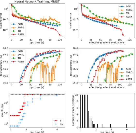
Neural Network Training
Finally, we also considered the problem of training a simple two layer feed-forward neural network on the popularMNIST data set of handwritten digits, see Lecun et al. (1998). Details concerning this data set can be found in Table A.1 in the appendix. The fully connected two layer neural network has 748 input neurons, 100 hidden neurons and 10 output neurons. The hidden neurons implement the logistic function, the output neurons the softmax function. Thus, if we have a data set (zi, y
i) ∈R784× {0,1}10, i = 1, . . . , n,
and choose the cross-entropy loss function, we arrive at the optimization problem min x∈Rm F(x) :=− n X i=1 10 X j=1 yjiln([h(zi, x)]j),
where h(·, x) denotes the function that implements the neural network with weight vector x.
In Figure 4.5 one can observe that ASTR achieves better results than the other methods concerning the training error. With regard to the test accuracy, ASTR performes on par with the tuned SGD method.