Sliding mode robot controller parameter tuning with genetic algorithms and fuzzy logic

SLIDING MODE ROBOT CONTROLLER PARAMETER TUNING

WITH GENETIC ALGORITHMS AND FUZZY LOGIC

by

Basel ELTHALATHINY

Submitted to the Graduate School of Engineering and Natural Sciences

in partial fulfillment of

the requirements for the degree of

Master of Science

Sabanci University

January 2013

ii

SLIDING MODE ROBOT CONTROLLER PARAMETER TUNING

WITH GENETIC ALGORITHMS AND FUZZY LOGIC

APPROVED BY:

Assoc. Prof. Dr. Kemalettin ERBATUR

………..

(Thesis Advisor)

Assoc. Prof. Dr. Ali KOŞAR

………..

Assoc. Prof. Dr. Volkan PATOĞLU

………..

Assist. Prof. Dr. Kemal KILIÇ

………..

Assist. Prof. Dr. Gürdal ERTEK

………..

iii

© Basel ELTHALATHINY

2013

iv

SLIDING MODE ROBOT CONTROLLER PARAMETER TUNING WITH GENETIC ALGORITHMS AND FUZZY LOGIC

Basel ELTHALATHINY

Mechatronics Engineering, Ms. Thesis, 2013

Thesis Supervisor: Assoc. Prof. Dr. Kemalettin ERBATUR

Keywords: Sliding Mode Control, Fuzzy Logic, Genetic Algorithms, Direct Drive Robots

ABSTRACT

Sliding Mode Controllers (SMC) possess robustness properties under parameter uncertainties. Usually, a Lyapunov based controller design with a switching control signal constitutes the backbone of robustness. However, the ideally zero switching time of the controller output cannot be achieved in digital implementation. This causes a phenomenon called chattering – high frequency oscillations observed in systems state variables. Chattering also shows itself as high amplitude oscillatory behavior in the control signal. A chattering actuator output is not favorable for many plants, including robot manipulators driven by actuator torques. This problem is traditionally solved by smoothing the switching control output, deviating from the original mathematical foundations robustness. Over-smoothing causes performance deterioration, while too limited smoothing action may lead to the wear of the mechanical system components. This motivates the exploration of automatic tuning approaches which consider chattering and performance simultaneously.

This thesis proposes two SMC smoothing and parameter tuning methods with soft computing (SC) methodologies.

The first method is based on Genetic Algorithms (GA). SMC controller parameters, including the ones governing the smoothing action are tuned off-line by evolutionary computing. A measure is employed to assess the instantaneous level of chattering. The

v

integral of this value combined with performance indicators including the rise time and steady state error in a step reference scenario are used as the fitness function. The method is tested on the model of a direct drive (DD) SCARA type robot, via simulations.

The GA-tuned SMC is, however, tailored for a fixed reference signal and fixed payload. Different references and payload values may pronounce the chattering effects or lead to performance loss due to over-smoothing. The second SMC parameter tuning method proposed employs a fuzzy logic system to enlarge the applicability range of the controller. The chattering measure and the sliding variable are used as the inputs of this system, which tunes the controller output smoothing mechanism on-line, as opposed to the off-line GA technique. Again, simulations with the direct-drive robot model are employed to test the control and tuning method.

vi

GENETĐK ALGORĐTMALAR VE BULANIK MANTIK ĐLE KAYAN KĐPLĐ ROBOT KONTROLÖRÜ PARAMETRE AYARLAMASI

Basel ELTHALATHINY

Mekatronik Mühendisliği Programı, Master Tezi, 2012

Tez Danışmanı: Doç. Dr. Kemalettin ERBATUR

Anahtar Kelimeler: Đnsansı robotlar, iki bacaklı yürüme referansı oluşturulması, iki bacaklı yürüme biçimi ayarlanması, genetik algoritma

ÖZET

Kayan Kipli Denetleyiciler (KKD) parametre belirsizlikleri karşısında gürbüzlük özelliklerine sahip denetleyicilerdir. Söz konusu gürbüzlüğün temelinde genellikle anahtarlamalı bir kontrol sinyali üreten Lyapunov tabanlı bir denetleyici tasarımı bulunmaktadır. Bununla beraber, ideal koşullarda söz konusu denetleyici tarafından sıfır zamanda anahtarlama yapan bir sinyal olarak üretilmesi beklenen kontrol çıktı sinyali sayısal uygulamada gerçekleştirlememektedir. Bu durum, çatırdama adı verilen ve sistem durum değişkenlerinde yüksek frekanslı salınımlara sebebiyet veren bir durum meydana getirmektedir. Çatırdama aynı zamanda denetleyici sinyalinde de yüksek genlikte salınımlı bir davranış şeklinde kendini göstermektedir. Çatırdamalı bir eyleyici çıktı sinyali, eyleyici torkları tarafından sürülmekte olan robot manipülatörler de dahil bir çok tesis için istenmeyen bir durumdur. Bu problem geleneksel yöntemlerde, denetleyicinin gürbüzlük özelliğini azaltmasına rağmen, anahtarlamalı denetleyici çıktı sinyalinin düzgünleştirilmesi yoluyla çözülmektedir. Fazla düzgünleştirme performans azalmasına, çok sınırlı düzgünleştirme ise mekanik sistemin komponentlerinde aşınma etkisine sepeb olabilmektedır. Bu etkenler, çatırdama ve performans etkilerini eş zamanlı bir şekilde ele alan otomatik ayarlama yaklaşımlarını motive etmektedir.

vii

Bu tezde, esnek hesaplama yöntemleri kullanan iki farklı KKD düzgünleştirme ve parametre ayarlama yöntemi önerilmektedir.

Birinci yöntem Genetik Algoritma (GA) tabanlı bir yöntemdir. Bu yöntemde, düzgünleştirme eylemini kontrol edenler de dahil, tüm KKD parametreleri evrimsel hesaplama kullanılarak çevrim dışı bir şekilde ayarlanmaktadır. Anlık çatırdama seviyesinin belirlenmesi amacıyla bir ölçüt kullanılmaktadır. Bu ölçütün integrali yanısıra, bir adım girdisi karşısındaki yükselme süresi ve kararlı durum hatası gibi performans göstergeleri form fonksiyonu olarak kullanılmaktadır. Söz konusu yöntem, doğrudan tahrikli bir SCARA tip robot manipülatör modeli kullanılarak gerçekleştirilen simülasyonlar üzerinde test edilmiştir.

Bununla birlikte, Genetik Algoritma tabanlı KKD, sabit bir referans sinyali ile sabit bir görev yükü için uygundur. Bu nedenle, farklı referanslar ve farklı görev yükü değerleri çatırdama etkilerini ortaya çıkarabilir veya fazla-düzgünleştirme temelli performans düşüşlerine neden olabilirler. Önerilen ikinci KKD parametre ayarlaması yöntemi, denetleyicinin uygulama alanını genişletme amaçlı bir bulanık mantık sistemi kullanmaktadır. Çevrim dışı çalışan GA yönteminin aksine bu yöntemde çatırdama ölçütü ve kayan değişken, anahtarlamalı denetleyici çıktısını çevrim içi olarak düzgünleştiren bu sisteme girdi olarak kullanılmaktadır. Aynı şekilde, doğrudan tahrikli robot model simülasyonları, geliştirilen denetleme ve ayarlama yönteminin test edilmesi için kullanılmıştır.

viii

To my beloved family ..

To my beloved mother ..

To my beloved Turkish wife ..

To my beloved aunts and cousins ..

To my beloved late father, Dr. G. ElThalathiny ..

To the Martyrs and Victims of the Arab Spring Revolutions ..

And specially the brave and blessed Martyrs of the Syrian Revolution ..

To Gaza .. and to its Martyrs, Victims, and People ..

To Palestine .. To Turkey ..

ix

ACKNOWLEDGMENTS

I would like to express my great thanks and gratitude to my beloved Thesis Supervisor, Dr. Kemalettin Erbatur, for his continuous support and caring .. For the hours he spent with me during the course work of this Thesis .. For the nights we spent in the laboratory, in his office, and in my office, while working together on this project .. I am so much grateful for all his efforts. No matter what I would say, I would never be able to express how grateful I am to his efforts and support. Thank you Sir.

I would like to thank both Dr. Kemal Kılıç and Dr. Gürdal Ertek for their continuous support either during my enrolment time at Sabanci University for the studies of my first Master Degree in the Industrial Engineering program, or after I left the university. They never hesitated to share their valuable time with me whenever I needed their advices. They cared about me and about my studies sincerely and professionally. They kept doing it even after I left the university and up till now. I am grateful for both of them. Dr. Kılıç was not just an advisor or just a professor, but rather was a true friend, true elder brother, and a very professional professor in his advices. Dr. Ertek was always there for me whenever I needed him. He shared long hours of his valuable time with me advising me, and showed true caring feelings towards my academic future and social life. Sometimes he worried about me, more than myself even. I am blessed to know him.

I would like to thank Dr. Güllü Kızıltaş Şendur for her academic support and advices. I would like to thank Dr. Cleva Ow-Yang for her professional advices.

I would like to thank Dr. Asif Şabanoviç for his efforts that helped me to get my Erasmus scholarship, and all his advices and efforts during the last 2 or 3 years, which guided me in my studies.

I would like to thank my family, my mother, my Turkish wife, and everyone who helped me during those long years of studies at Sabanci University. Thank you all. I love you all. I care about you all.

Also, I would like to thank all my friends and colleagues for their warm feelings. Out of those, I would like to thank Dr. Islam Shoukry Mohammed Khalil, who is a Master and a

x

Ph.D. Alumni of the Mechatronics Engineering Department at Sabanci University, and who explained and taught me a lot of things to me during my courses in the program. Also, Abdullah Kamadan was very helpful and true advisor and brother in many situations. Of course I would like to thank my colleague Iyad Hashlamon who’s that much close to get his Ph.D. degree in Mechatronics Engineering from Sabanci University. He was always there whenever I needed him to explain some parts of the courses I took. He shared his time generously and never hesitated to offer all the help and support he could offer. Thank you my dear friend and I was blessed to know you. Thank you indeed.

xi

SLIDING MODE ROBOT CONTROLLER PARAMETER TUNING WITH GENETIC ALGORITHMS AND FUZZY LOGIC

TABLE OF CONTENTS

ABSTRACT ... iv

ÖZET ... vi

ACKNOWLEDGMENTS ... ix

TABLE OF CONTENTS ... xi

LIST OF FIGURES ... xiii

LIST OF TABLES ... xvi

LIST OF SYMBOLS ... xvii

LIST OF ABBREVIATIONS ... xix

1. INTRODUCTION ... 1

2. A SURVEY ON SLIDING MODE CONTROLLERS, GENETIC ALGORITHMS AND FUZZY LOGIC SYSTEMS ... 4

2.1. Sliding Mode Control ... 4

2.2. Genetic Algorithms ... 7

2.3. Fuzzy Logic Systems ... 10

2.4. SMC with GA ... 11

2.5. SMC with FL ... 12

3. THE SCARA-TYPE DIRECT-DRIVE TWO-DEGREES-OF-FREEDOM ROBOT ... 15

4. THE SLIDING MODE CONTROL METHOD ... 19

4.1. Sliding Mode Controller ... 19

4.2. Application of the SMC to the Direct Drive Robot ... 23

4.3. Sliding Mode Controller with Modified Controller Gain for Smoothing ... 27

5. GENETIC TUNING OF THE SMC ROBOT CONTROLLER ... 32

xii

5.2. The Fitness Function ... 33

5.3. GA Parameters ... 35

5.4. Results of the Tuning Process ... 36

6. SMC ON-LINE PARAMETER ADJUSTMENT BY A FUZZY LOGIC SYSTEM ... 42

7. CONCLUSION ... 60

xiii

LIST OF FIGURES

Figure 2.1: A sample Cross-Over ... 8

Figure 2.2: Mutation ... 9

Figure 2.3: Reproduction Scheme ... 9

Figure 2.4: Basic Pure Fuzzy Logic Systems Structure ... 10

Figure 2.5: Fuzzy Logic System Basic Structure with a Fuzzifier and a Defuzzifier ... 11

Figure 3.1: The CAD Models of the direct drive SCARA type robot arm and link ... 17

Figure 3.2: The description of the Robot joint angle and length parameters ... 17

Figure 4.1: The Sliding Line ... 21

Figure 4.2: Sliding mode control without control signal smoothing. Joint positions, step position references and control torques for the base and elbow are shown ... 25

Figure 4.3: Sliding mode control without control signal smoothing Phase plane trajectories for the base and elbow joints. The dashed lines are the sliding surfaces . ... 26

Figure 4.4: The smoothing function

ρ

₁ for the base joint control signal ... 27

Figure 4.5: Sliding mode control with control signal smoothing. Joint positions, step position references and control torques for the base and elbow are shown ... 29

Figure 4.6: Sliding mode control with control signal smoothing. Phase plane trajectories for the base and elbow joints. The dashed lines are the sliding surfaces. ... 30

Figure 4.7: Smoothing functions

ρ

₁ and

ρ

₂ obtained by trial and error and used for the results presented in Figures 4.5 and 4.6. ... 31

Figure 5.1: Convergence of the fitness function. The first six plots are components of the combined fitness function shown in the last plot ... 37

xiv

Figure 5.2: GA tuned sliding mode control with control signal smoothing. Joint positions, step position references, control torques and chattering variables for the base and elbow are shown. Note that GA turning is applied for the base joint only ... 38 Figure 5.3: GA tuned sliding mode control with control signal smoothing. Phase

plane trajectories for the base and elbow joints. The dashed lines are the sliding surfaces. Note that GA tuning is applied for the base joint only ... 39 Figure 5.4: Smoothing function

ρ

₁ obtained via GA tuning. ... 40 Figure 6.1: GA tuned sliding mode control with control signal smoothing with

larger step references than used in the tuning process. Joint positions, step position references, control torques and chattering variables for the base and elbow are shown. Note that GA tuning is applied for the base joint only. ... 43 Figure 6.2: GA tuned sliding mode control with control signal smoothing with

larger step references than used in the tuning process. Phase plane trajectories for the base and elbow joints. The dashed lines are the sliding surfaces. Note that GA tuning is applied for the base joint only .. 44 Figure 6.3: GA tuned sliding mode control with control signal smoothing with

larger payload than used in the tuning process. Joint positions, step position references, control torques and chattering variables for the base and elbow are shown. Note that GA tuning is applied for the base joint only . ... 45 Figure 6.4: GA tuned sliding mode control with control signal smoothing with

larger payload than used in the tuning process. Phase plane trajectories for the base and elbow joints. The dashed lines are the sliding surfaces. Note that GA tuning is applied for the base joint only ... 46 Figure 6.5: The membership functions ... 49

xv

Figure 6.6: GA tuned sliding mode control with control signal smoothing with the same size of step references and same payload used during the GA process. Fuzzy adaptation is active. Note that GA and fuzzy tuning are applied for the base joint only ... 52 Figure 6.7: GA tuned sliding mode control with control signal smoothing with the

same size of step references and same payload used during the GA process. Fuzzy adaptation is active. Note that GA and fuzzy tuning are applied for the base joint only ... 53 Figure 6.8: GA tuned sliding mode control with control signal smoothing with 2 rad

step references and same payload used during the GA process. Fuzzy adaptation is active. Note that GA and fuzzy tuning are applied for the base joint only ... 54 Figure 6.9: GA tuned sliding mode control with control signal smoothing with 2 rad

step references and same payload used during the GA process. Fuzzy adaptation is active. Note that GA and fuzzy tuning are applied for the base joint only ... 55 Figure 6.10: GA tuned sliding mode control with control signal smoothing with the

same size of step references used during the GA process and 15 kg payload. Fuzzy adaptation is active. Note that GA and fuzzy tuning are applied for the base joint only ... 56 Figure 6.11: GA tuned sliding mode control with control signal smoothing with the

same size of step references used during the GA process and 15 kg payload. Fuzzy adaptation is active. Note that GA and fuzzy tuning are applied for the base joint only ... 57 Figure 6.12: GA tuned sliding mode control with control signal smoothing with 2

rad step references and 15 kg payload. Fuzzy adaptation is active. Note that GA and fuzzy tuning are applied for the base joint only ... 58 Figure 6.13: GA tuned sliding mode control with control signal smoothing with 2

rad step references and 15 kg payload. Fuzzy adaptation is active. Note that GA and fuzzy tuning are applied for the base joint only ... 59

xvi

LIST OF TABLES

Table 2.1: The parameters of GA ... 9

Table 3.1: Robot Dynamics Parameters ... 18

Table 4.1: Controller Parameters ... 25

Table 4.2: Controller and Control Smoothing Parameters ... 31

Table 5.1: The Chromosome Structure ... 33

Table 5.2: The Coefficients used in the Fitness Function ... 35

Table 5.3: GA parameters ... 35

Table 5.4: The GA Tuning Results ... 40

xvii

LIST OF SYMBOLS

i

x : The State Vector.

) (ki

i

x : The kith derivative of xi.

u : The Control Input.

B : The Gain Matrix. s : The Sliding Function.

d

x : The Desired State Vector.

G : The Slope Matrix of the Sliding Surface.

i

e : The Error for xi. i

s _{: The} th

i component of the Sliding Function s. )

(s

V : The Lyapunov Function.

sign(s) : The Vector Signum Function. )

(t

u_{eq : The Equivalent Control Term.}

1

J &J₂ : The Rotor Inertia Values of the Base and Elbow Joints.

D : The Inertia Matrix of the Manipulator. 1

q : The Angular Position of the Base Joint. 2

q : The Elbow Angular Position.

C : The Matrix for Centripetal and Coriolis effects. 1

B &B₂ : The Constant Coefficients of the Viscous Friction of the 2 Joints.

1

c

F &F_c2 : The Torques of the Coulomb Friction. M

J : The Manipulator Jacobian.

x e F &

y e

F _: The Components of the Exerted Force on the Environment by the Tip of the Manipulator.

1

τ &τ₂ : The Joint Actuation Torques. 1

I &I₂ : The Base and Joint Links Inertia. 1

xviii i

Bˆ : The Viscous Friction. i

K : The Controller Corrective Gains.

1 1 ε , 1 2 ε , 1 3 ε , 1 1 η & 1 2 η

: The Parameters define the Function

ρ

₁.

1

ψ

: The Scaling Variable.

xix

LIST OF ABBREVIATIONS

2-D : Two Dimensional. 3-D : Three Dimensional.

CAD : Computer-Aided Design OR Computer-Aided Drafting. DD : Direct Drive.

DoF : Degrees of Freedom. DSP : Digital Signal Processing. dSPACE : Name of a Software Package. FL : Fuzzy Logic.

GA : Genetic Algorithm.

MIMO : Multiple-Input and Multiple-Output. NB : Negative Big.

NN : Neural Network. NS : Negative Small. PB : Positive Big.

SCARA : Selective Compliant Assembly Robot Arm OR Selective Compliant Articulated Robot Arm.

SISO : Single-Input and Single-Output. SMC : Sliding Mode Control.

1

Chapter 1

1. INTRODUCTION

It is not easy at all to handle robot manipulator control due to nonlinear and coupled system dynamics. Usually, system parameters in motion control applications are unknown or they may vary with time; but Sliding Mode Control – shortly known as SMC – copes with the changing parameters and nonlinearity problem. This is true even when what we know about plant dynamics is limited, which makes SMC a robust control strategy.

[1] and [2] state that SMC was firstly introduced in the 50’s of the 20th century, but it received more attention in the 70’s of the same century, and since then, it has been employed in a huge variety of applications. Those include motion control, chemical plant control, converters of power, and robotics [3-4].

SMC is very well known and mostly famous with its robustness as its most attractive property, because once we force the system to be in a sliding mode, disturbances and parameter changes no more affect it.

The control signal of the SMC is discontinuous, and it switches over a predefined region in what is known as the state space. To have all motions in this region neighborhood directed towards the region, it is certainly required to have some conditions met, so we can end up by having the results towards zero in any sliding motion of the states that follow the dynamics, which were defined by its region [5]. Usually the sliding region is nothing but a line in a 2-D state plane. We have the system in the sliding mode only when the state variables move on the sliding region. Such a mode provides us with many useful properties that enable us to track the control of the uncertain nonlinear systems, which make it full of properties that can be described as invariance ones when it comes to the uncertainties we may face in the plant model itself. For more information about such a thing, a survey of sliding mode controllers was provided in [6]. [7-11] confirm that Robotics is indeed an area where SMC can be applied successfully.

2

In spite of that, and unfortunately, Sliding Mode Controllers are very well known by some problems that may have some significant effects on the system. The most significant one is what is known as “Chattering”, which is the oscillations of the controller output. Another one would be the huge employment of unnecessarily large control signals in order to override the uncertainties of the parametric. “The amount of control necessary to keep the system state variable on the sliding region”, which is the equivalent control, cannot be easily calculated; thus, a full knowledge of the plant dynamics is a must [12]. Previously, many modifications have been proposed to the pure sliding control law to ease handling such problems [13]

The huge developments in the fields known as the Intelligent Control, the Fuzzy Logic, and the Evolutionary Computing approaches, gave huge flexibility to the designers of the systems to overcome the uncertainty problems by either learning from their experience or by implementing their own understanding of the problem [14-15]. Some of the results of these researches were reported in [16-33].

One of those techniques is known as the Genetic Algorithms, which is used to explore search spaces with large dimensions by imitating the process of evolution in nature. Stronger Individuals (solutions) according to specifically designed fitness criterion survive to pass their “Genetic Material”, which is/are (a) suitable part(s) of the solution, to the individuals existing in the next generation. Continuous iterations of the new generations provide us some kind of an optimized solution that we can code in the “Chromosome” of what is known as the “Test Winner” in the last generation. By this, we can consider GA as suitable tools for the adjustment of many nonlinear controllers’ parameters indeed.

On the other hand, Fuzzy Logic systems employ human experience into the control task as one of the many other intelligent control techniques. Fuzzy Rules are used to compute the control signal in the control process of the robotic trajectory. Also, the other controllers parameters can be tuned on-line by using them, which enable us to reach a better performance when we have uncertainties and operating points that do vary.

This thesis proposes two SMC smoothing and parameter tuning approaches.

The first approach is based on GA. In this method, various SMC controller parameters are tuned off-line by evolutionary computing. The parameters used to describe a control output smoothing mechanism are among the tuned ones. The sliding region - a sliding line in this case - is also adjusted by the GA system, along with the main coefficient of the control action, which

3

pushes system state variables towards the sliding line. A chattering measure is introduced. The integral of the sliding measure, and performance indicators, including the rise time, error integral and steady state error, are used to define a fitness function in a step reference scenario. The method is tested on the model of a 2-DoF DD (Direct Drive) SCARA type robot, via simulations. The GA-tuned SMC, however, is obtained for a fixed reference signal and fixed payload. Different references and payload values may lead to chattering effects and performance degradation. The second SMC parameter tuning method proposed in the thesis employs a fuzzy logic system to enlarge the operation range of the controller. The chattering measure and the sliding variable are used as the inputs of this system. The fuzzy logic system tunes the controller output smoothing mechanism on-line, which opposes the off-line GA technique. Again, simulations carried out with the Direct-Drive robot model are employed to test the control and the tuning method. The variable sliding control gain and the introduction of a “Smoothing Function” tuned by a GA and a Fuzzy Logic System are novel contributions.

The thesis is organized as follows. The second chapter outlines principles of sliding mode controllers, genetic algorithms and fuzzy logic systems. Practical difficulties and popular solutions are discussed for sliding mode controllers. A survey on the combination of GA and fuzzy systems with sliding mode controllers is also presented. The direct-drive SCARA type robot model used in this study is introduced in Chapter 3. Chapter 4 is devoted to the description of the particular SMC employed in the thesis. The GA based tuning of this controller is presented in Chapter 5, and Chapter 6 discusses the fuzzy logic on-line tuning system. Developments in Chapters 4, 5, and 6, are accompanied by simulation results with the robot model. Conclusions and a discussion of future work are presented in the last chapter.

4 Chapter 2

2. A SURVEY ON SLIDING MODE CONTROLLERS, GENETIC ALGORITHMS AND FUZZY LOGIC SYSTEMS

In this chapter, a survey on the integration of GA and fuzzy logic systems with SMC is presented. The first three subsections are devoted to outline the basic principles of SMC, GA, and fuzzy logic, as separate methodologies.

2.1. Sliding Mode Control

In order for the system to stay in a “sliding mode”, and thus, it will not be affected by disturbances and modeling uncertainties; error states in SMC should be driven to the

“switching/sliding” surface. By definition, the control of an (n−1)st-order system is much easier

than the control of an nth-order system. The basics of Sliding Mode Controller design are

outlined below to support the discussions in the following chapters. The approach mentioned below was chosen carefully to provide a framework for the coming discussions. However, a variety of other SMC designs are provided in the literature. This approach provides an example to present the difficulties of the Sliding Mode Controllers tackled in some practical applications.

The plant under consideration is a nonlinear MIMO system:

∑

= + = m j j ij i k i f x b u x i 1 ) ( ) ( i=1,...,m. _(2.1) ) (ki i

x here refers to the th

i

k derivative of x_i. The state vectors of the subsystems described in (2.1)

were combined to form the state vector x.

[

_k

]

T m m m k _{x x x} m x x x x 1 1 1 1 1 1− − = & L L & L _{. (2.2)}

5

[

]

T m u u u L 1 = . _(2.3)

Let x be (nx1), then we can express the system equation as

) ( ) ( ) (t f x Bu t x& = + _{. (2.4)}

Let B be the (nxm) gain matrix. Thus, the sliding surface will be defined as the surface where the

(mx1) variables, defined by ) ( ) ( )) ( ) ( ( ) , (x t G x t x t t s X s a d _{− = −} = & φ _{, (2.5)}

is equal to zero. s refers to the sliding variable (the sliding function).

In (2.5), ) ( ) ( s and ) ( ) (t ₌Gxd t _a x ₌Gx t φ . _(2.6)

They are nothing but the time and the state dependent parts of the sliding function, respectively. In (2.6), xd refers to the desired state vector, while G is the (mxn) slope matrix of the sliding

surface. G was chosen so that the sliding surface function can be represented as

i k i i e dt d s i−1       ₊ = λ . (2.7) i

s is the ith component of the sliding function s. e_i refers to the error for x_i defined by

i d i

i x x

e = − . _(2.8)

The constants λ_i were selected positive. We know that the error e_i converges to zero if si equals

zero. Generally, the errors of the system converge to zero, if the states are on the sliding surface (with the error dynamics defined by the sliding surface parameters).

The SMC design was formed by Lyapunov function selection. The control law is to be chosen so that a Lyapunov function candidate satisfies criteria of stability of Lyapunov. Thus, the Lyapunov function candidate was chosen as

2 ) (s s s V T = . _(2.9)

6

Now we have a positive definite function. It is desired to have the derivative of the Lyapunov function as a negative definite. It is doable if

) ( sign ) ( s D s dt s dV ₌₋ T (2.10)

of some mxm positive definite diagonal gain matrix D. sign(s) refers to the vector signum

function. sign(s_i) affects the components of s. It is defined as

   < − > + = 0 1 0 1 ) ( sign i i i s s s . _(2.11)

By differentiating (2.9), and then equating it to (2.10), we obtain

) ( sign s D s dt ds sT =− T . _(2.12)

Let’s take the time derivative of (2.5), and let’s use the plant equation to reach

) ) ( (f x Bu G dt d dt dx x s dt d dt ds _a + − = − =

φ

∂

∂

φ

. _(2.13)

Place (2.13) into (2.12) to get the control input signal as

) ( ) ( ) (t u t u t u = _eq + _c , _(2.14)

and u_eq(t) is nothing but the equivalent control term given by

      ₋ − = − dt t d x Gf GB t u_eq( ) ( ) 1 ( )

φ

( ) , _(2.15)

while u_c(t) is a corrective control defined as

) ( sign ) ( sign ) ( ) (t GB 1D s K s u_c = − ≡ . (2.16)

Just for the record, we do have many other choices for both the Lyapunov function and the desired derivative of it. However, each one of them will definitely yield some different forms for the corrective control term.

As it was stated before in Chapter 1, the pure form of the SMC does suffer from some drawbacks when it comes to real practical applications. One of them is the controller output high

7

frequency oscillations known as chattering. The ideally infinite frequency switching necessary for the sliding mode establishment causes such oscillations. In addition to the fact that chattering may cause severe damages to the mechanical components, the instability resulted by the high frequency plant dynamics, which may be excited by Chattering, is definitely undesirable in almost all implementations.

Moreover, an SMC is easily vulnerable to the measurement noises, which makes it a 2nd

problem. Measurement noise has very negative effects when the measured sliding variable is close to zero, but control signal depends on the sign of it measured there.

The 3rd problem is due to the fact that the SMC can employ too large control signals to

overcome the uncertainties of the parameters.

The 4th problem is the difficulty to calculate the equivalent control, which demands us

to endorse a complete knowledge of the plant dynamics.

In order to overcome those problems, some modifications to the original sliding control law had to be suggested and implemented [34]. One of those modifications is the Boundary Layer approach. In the place of the signum function, a saturation function is implemented [7, 12]. Another one would be the “Provident Control”. It just switches between control structures to avoid a sliding mode [35, 36]. A good mathematical model of the plant is required for the computation of the equivalent control. [37] proposed the use of an equivalent control estimation technique.

2.2. Genetic Algorithms

Genetic Algorithms (GA) are heuristic methods employed to solve complex optimization problems [38]. They use the "Survival of the Fittest" principle and compare candidate solutions according to their fitness. Fitness can be as a measure of qualities or disadvantages of the solution. A solution is coded into registers called "Chromosomes" after the analogy with living beings. A set of solutions - called a population - is created randomly at first. The solutions are called individuals of this population. Individuals are then ranked according to their fitness values. The next generation of the population is created from the first generation by chromosome cross-over and mutation processes. Chromosomes of fitter individuals are favored in this mechanism to pass their contents into the next generation. The candidates chosen for this

8

process are called parents. Usually the parents are selected randomly using a scheme which favors the more fit individuals. After the selection process, their chromosomes are recombined. The process of producing offspring individuals creates the next generation. In traditional GA, crossover and mutation are the two typical mechanisms. The crossover and mutation operators are used on randomly selected parents from the candidate pool. Also to reduce the probability of

divergence, a number of elite (the fittest) members of each population are transferred to the next

one. New generations are created iteratively. A solution individual with the desired value of fitness can be generated in this manner with a number of iterations [38].

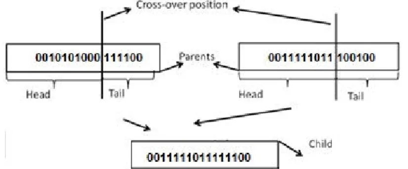
At some randomly chosen 2 positions of the chromosome strings of 2 individuals chosen randomly to let the crossover concentrates on them by dividing their chromosome strings

at those 2 positions, 4 produced segments are referred to them as tails and heads. The tail

segment of the first individual and the head segment of the second individual are combined to produce a new full length new chromosome. This is referred to as single point crossover. A crossover sample for the given parents is shown in Figure 2.1.

Figure 2.1: A sample Cross-Over

Individuals chosen in a random manner suffer from an enforced mutation after the crossover by altering a randomly chosen gene, in order to avoid local solutions by at random search [38]. Figure 2.2 shows the mutation operation of an individual.

9

Figure 2.2: Mutation

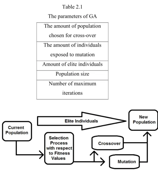
Then the individual’s number within the population and the maximum iterations will be set because they are very important parameters of the GA methodology. In addition to the percentages of the population selected for crossover and mutation, the percentage of the elite members (They will pass directly to the next generation) is another important parameter of the GA methodology. The parameters of the GA methodology are shown in Table 2.1, while the overall Reproduction Operation is shown in Figure 2.3.

Table 2.1 The parameters of GA The amount of population

chosen for cross-over The amount of individuals

exposed to mutation Amount of elite individuals

Population size Number of maximum

iterations

10

2.3. Fuzzy Logic Systems

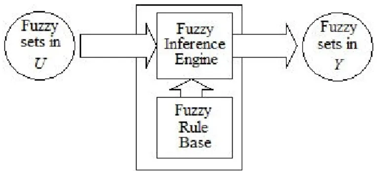
Figure 2.4 shows a basic pure fuzzy logic system diagram. From it, it is clear that the Fuzzy Rule Base consists of a set of fuzzy IF-THEN rules to determine a mapping from the fuzzy sets in the input discourse U universe to fuzzy sets in the output discourse Y universe based on the principles of the fuzzy logic.

Figure 2.4: Basic Pure Fuzzy Logic Systems Structure.

In this scheme the fuzzy IF-THEN rules are of the form

l l n n l l G y F x F x

R :IF 1is 1 and and is THEN is

) (

L _(2.17)

l i

F and Gl are fuzzy sets, x=(x_1,K,x_n)∈U _{and y}∈_{Y are input and output linguistic}

variables, respectively, and l =1,2,K,M _{, where M is the number of rules. This type of fuzzy}

systems provides a good framework to incorporate human expert’s knowledge in it, yet, it has a disadvantage of having fuzzy sets as inputs and outputs whereas the variables in engineering applications may vary and they are real-valued.

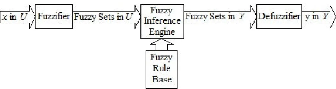
Figure 2.5 shows fuzzy logic systems basic structure with Fuzzifier and Defuzzifier. Inputs and outputs are real-valued variables in engineering systems. Thus, to use the pure fuzzy logic system shown in Figure 2.4 above in engineering systems, adding a Fuzzifier and a Defuzzifier to the input and output of the system, respectively, is the most straightforward way. Crisp values into fuzzy sets are mapped by the Fuzzifier, while fuzzy sets to crisp values in the output section are mapped by the Defuzzifier. Nevertheless, and due to the fact that they are in a

11

pure fuzzy logic system, the fuzzy rule base and the inference engine remain unchanged. Mamdani was the first to propose such kind of fuzzy logic system [39] and he applied it successfully to many control problems. Fuzzy logic systems accompanied by a Fuzzifier and a Defuzzifier have a lot of advantages, which makes them suitable for engineering applications due to the crisp input and output values. They really do constitute some kind of a natural framework to incorporate human knowledge to the problem by having many choices for the Fuzzifier, the Inference Engine, and the Defuzzifier, to obtain the most suitable system for a specific problem under testing. There are many training algorithms that can be developed widely to specify the parameters of these systems.

Figure 2.5: Fuzzy Logic System Basic Structure with a Fuzzifier and a Defuzzifier.

2.4. SMC with GA

The integration of GA and VSS control has some kind of an indirect nature. GA tune the control parameters of the VSS based on many reports in the literature. 2 examples on the use of GA in SMC construction were presented in [40]. In [41], a Fuzzy SMC structure was taken into consideration. In this structure, the consequents were control outputs and the antecedents were fuzzy sets on the sliding variable. Also, 2 kinds of GA-based fuzzy SMC design methods

were studied. In the 1st kind, only the parameters in the THEN part were known, while in the 2nd

kind, all the parameters in both the IF part and the THEN part were taken into consideration. Đn [42], in order to reduce chattering, GA were used to estimate the required magnitude of the switching control. In [43], GA was used in the computation of the most suitable membership functions for a smoother fuzzy SMC. Parameters of the controller were obtained by a GA by a SMC design in [44]. In [45], a reluctance motor optimal speed control was carried out where a GA system was used to search for the uncertain parameters.

12

2.5. SMC with FL

Đf we have some implementation difficulties of the SMC, we can use a Fuzzy Logic alongaside a SMC to solve them by adding a Fuzzy Logic system. While it is true that the basic design and implementation of SMC is followed, but Fuzzy Logic systems are used to play a secondary role. Their implementation would be either to adapt the controller parameters, to handle the elimination process of the chattering, or to tackle the problems of modeling

difficultueis and the calculations difficulties of the control u_eq.

We can use a low pass filter as a common approach to prevent chattering by smoothing the control input in a SMC. If the filter bandwith is small, abrupt changes in the control signal can be prevented. But, if the filter bandwith is too small, the difference between the original and the filtered control signals can be too large, and thus, we will have a more significant deviation of the system from the ideal sliding mode. If the state is kept within the closeness of the sliding

surface, then the bandwith shall be small, because the change in u will be expected to be abrupt.

In [16], a fuzzy system was used so that the bandwith was made large in order to maintain the advantages of the SMC.

[18] used sliding mode parameters tuning via fuzzy systems. A discrete-time fuzzy-sliding-mode controller applied to vibration control of a smart structure featuring a piezo film actuator was presented. Firstly, they considered a discrete-time model with mismatched uncertainties for the design of a discrete-time sliding-mode controller (it has two parts: an equivalent part and a discontinuous part). They employed a fuzzy technique to appropriately determine control parameters (discontinuous feedback gain was one of them) to formulate the fuzzy-sliding-mode controller, which was used in their experiments to demonstrate the effectiveness of the proposed method.

The design of SMC difficul task because an exact knowledge of the plant is rarely (if ever) available, and the bounds of the uncertainties may not be known. Thus, the use of an adaptive Fuzzy Logic identifiers for the uncertainties was proposed by many researchers. In [19], to adaptively model the plant non-linearities, which have unknown uncertainties, a fuzzy system architecture was employed, in which, the modeling error bound (results from the error between the actual nonlinear plant and the fuzzy system - an inverted pendulum system) is identified adaptively, and by using this bound, the sliding control input was calculated.

13

In [20], a non-linear system was firstly linearized around some operating points, and then, the Fuzzy Logic principles were used to aggregate each locally linearized model into a global model representing the non-linear system, then, a vigirous SMC was proposed to guarantee system asymptotic stability.

Fuzzy approximators in modeling uncertainties were also noticed [46, 47]. Both Fuzzy approximators and sliding control schemes were considered in [48], in which, 2 adaptive SMC schemes with fuzzy logic systems as approximators were designed. The Fuzzy Logic systems were used for the approximation of the unknown system functions. A fuzzy logic system

approximates the nonlinear system x&= f(x)+bu_{unknown function, then a robust adaptive law}

was employed to minimize the approximation errors between the real system functions and the fuzzy approximators in the first method; while in the second method, two fuzzy logic systems were used to approximate f and b, respectively. Stability proofs of the control schemes were given too.

To approximate the unknown dynamics in each sub-system of an interconnected nonlinear system, fuzzy logic systems were employed in [21]. In order to compensate for the fuzzy approximating errors and to attenuate the interactions between sub-systems, a fuzzy sliding mode controller was developed after that. With the tracking errors converging to a neighborhood of zero, a global asymptotic stability was established in the Lyapunov sense.

In [49], a decentralized adaptive fuzzy control scheme was employed to overcome difficulties caused by coupling effects for a class of large-scale nonlinear systems (large scale plants) with unknown constant control gains was proposed, which does not require detailed models and accurate load forecasting. Thus, an adaptive fuzzy control scheme was obtained using the principle of sliding mode control and the approximation capability of fuzzy systems. Fuzzy systems are universal approximators. This was considered in the structure design expressed in [46], which used decentralized fuzzy systems to approximate the controlled process and to adaptively compensate for the plant uncertainties. They used the Lyapunov function method to obtain a proof for global stability. Moreover, the simulation results presented indicated clearly strong robustness against both model uncertainties and nonlinear sub-system interactions. In addition to all of that, the tracking errors converged to a neighborhood of zero, and the proper fuzzy logic switchings that were applied ensured the avoidance of the chattering phenomenon inherent in sliding mode control.

14

[50] proposed modeling and control approaches for uncertain nonlinear dynamic systems using fuzzy set theory. A fuzzy-set based representation of the uncertain systems was developed for modeling. A robust control design was made feasible with neither resorting to model simplification, nor imposing restrictions on uncertainty and the fuzzy control design approach was developed with a fuzzy model representation of uncertain systems. To show usefulness of the method, a single-link robot arm with uncertain dynamics was used as a simulation test bed.

Fuzzy Logic systems can be considered as complementary controllers to SMC schemes by some approaches. At the start, Sliding Mode Controllers have to be designed. Then, additional fuzzy control terms are used together with the sliding mode controller output for performance enhancement and chattering elimination. [22] presented a similar scheme for linearized systems suffering from uncertainties. To compensate for the influence of the un-modeled dynamics and chattering, SMC combined with fuzzy tuning was used. Then in [23] this approach was further generalized to a class of nonlinear systems, where the simulations on a robotic manipulator were presented.

15 Chapter 3

3. THE SCARA-TYPE DIRECT-DRIVE TWO-DEGREES-OF-FREEDOM ROBOT The experimental manipulator used in the thesis is described in this Chapter. Figure 3.1 shows the 2-DoF Direct Drive manipulator built at the Robotics Laboratory of Sabanci University. The arm is controlled by a dSPACE 1102 DSP-based system. The user interface software ran on a PC and C language servo routines were compiled in this environment. Then they were downloaded to the DSP. To provide position measurement signals with a resolution of 1024000 pulses/rev, a Yokogawa Dynaserv direct drive motors were used at base and elbow joints. The torque capacity of the base motor was 200 Nm, while the one of the elbow motor was 40 Nm.

The robot dynamics equation is defined as

τ τ τ =       =         +       +                   + +             +       2 1 2 1 2 1 2 1 2 1 2 , 1 2 1 2 1 2 1 0 0 ) , , ( ) , ( 0 0 y x e e T M c c F F J F F q q B B q q q q C q q q q D J J & & & & & & & & , (3.1)

where J₁ and J₂ represent the rotor inertia values of both the base and the elbow joints,

respectively. D is the inertia matrix of the manipulator. q₁ is the angular position of the base

joint. q₂ is the elbow angular position shown in Figure 3.2. C refers to the matrix for centripetal

and Coriolis effects; while B₁ and B₂ are the constant coefficients of the viscous friction of the

two joints. F_c1 and F_c2 refers to the torques of the Coulomb friction. J_M is the manipulator Jacobian, but it is restricted to two dimensions in (3.1), and it is a 2×2 matrix relating the 2-dimensional linear Cartesian velocity to the 2-2-dimensional vector of the joint velocity.

x e

F and

y e

F are the components of the exerted force on the environment by the tip of the manipulator

tool, expressed in the x and y axis directions of the base frame of the robot. The joint actuation

torques τ₁ and τ₂ control the robot. Actually, there is no gravity effect acting on the joints, simply

because of the arrangement of the horizontal kinematic of the robot. The matrices C and D are

16       + + + + + + + + + + = 2 2 2 2 2 2 2 1 2 2 2 2 2 2 1 2 2 2 2 1 2 2 1 2 2 2 1 2 2 1 1 2 1 ) cos ( ) cos ( ) cos 2 ( ) , ( I l m I q l l l m I q l l l m I I q l l l l m l m q q D c c c c c c c c (3.2) and      − − + = 0 ) ( ) sin ( ) , , , ( 1 2 1 2 2 2 1 2 2 1 2 1 q q q q q l l m q q q q C _c & & & & & _{. (3.3)}

The various parameters of the link length, mass, and inertia, shown in (3.2) and (3.3), are described in Table 3.1. By using the CAD models of the links shown in Figure 3.1. Link inertia parameters and center of mass locations were computed. Link lengths and joint to center of mass distances (l₁,l₂) are indicated in Figure 3.1. The values of the link inertia I₁ and I₂ were computed about the axes perpendicular to the sketch plane and run through the center of mass

points c₁ and c₂ shown. The values of the rotor inertia J₁ and J₂ were taken from the

manufacturer’s documentation. We got (3.2) and (3.3) with the Euler-Lagrange method [52]. By using the parameters in Table 3.1, we obtained the numerical values of these expressions. Even though friction parameters, especially Coulomb friction, were difficult to model, but still, rough estimates of the coefficients of the viscous friction (Bˆ₁,Bˆ₂) were achieved experimentally by using force sensors. They are listed in Table 3.1.

17

Figure 3.1: The CAD Models of the direct drive SCARA type robot arm and link

18 Table 3.1

Robot Dynamics Parameters

Link 1 weight m₁ (including elbow motor) 17.9 kg Link 2 weight m₂ 3.25 kg Link 1 inertia I₁ (Including elbow motor) 0.54 kg m2 Link 2 inertia I₂ 0.04 kg m2

Motor 1 rotor inertia J₁ 0.167 kg m2 Motor 2 rotor inertia J₂ 0.019 kg m2

Link 1 length l₁ (Joint center to joint

center)

0.4 m

Link 2 length l₂ (Joint center to tool

center)

0.28 m

Link 1 joint to center

of mass distance l_c1 0.277 m

Link 2 joint to center of

mass distance l_c2 0.09 m

Joint 1 viscous friction coefficient Bˆ1

3 Nms/rad

Joint 2 viscous friction coefficient Bˆ2

0.6 Nms/rad

The next chapter describes the force control algorithm with the fuzzy logic controller scheduling.

19 Chapter 4

4. THE SLIDING MODE CONTROL METHOD

In this section, the SMC method which was used in this thesis is presented. Firstly a general SISO controller scheme will be briefed. Next, its application on the direct-drive SCARA arm will be considered and simulation results will be obtained with the switching controller. Finally, a controller smoothing mechanism will be proposed and will be simulated.

4.1. Sliding Mode Controller

Second order SISO systems were focused on. Systems with the following state equations form were considered

u X b X f x&= ( )+ ( ) & . (4.1)

X is an augmented vector of the scalar state variables x, x&

[

]

T

x x

X = & _{. (4.2)}

uis the control input. The input gain b(X) takes strictly positive values. The tracking error is

represented as

x x

e= _d − (4.3)

in which x_d represents the desired value of x. The sliding variable s is shown as

e e e

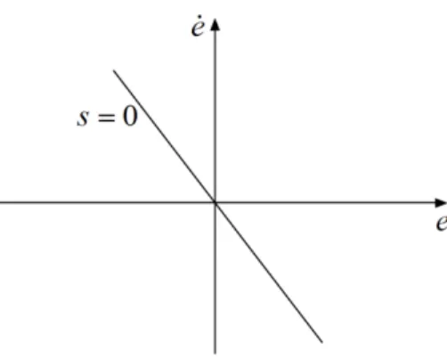
s_{( )}= &+λ _{. (4.4)}

For this system, the desired dynamic response is given by s =0. For stability, we introduced λ

as a positive number. If we can force s to zero, then we can attain the desired dynamics, and the

tracking error will converge to zero with the dynamics e&+λe=0_{, which represents a line with}

slope −λ in the phase plane as shown in Figure 4.1. In the literature, an approach which

involves the selection of a Lyapunov function V of s, is followed mostly. This function is chosen

20

2 2 1_s

V = . (4.5)

We need to construct a control law in such a way that the sliding line is attractive for the state trajectories on the phase plane. Thus, the closed loop system stability can be guaranteed, if the

derivative of Vis shown to be negative definite [12]. The Lyapunov function derivative is

s s

V& = &_{. (4.6)}

By using (4.1 – 4.4), we can represent this equation as, ) ) ( ) ( (x f X b X u e s

V &&d &

&_{= − − +λ}

. (4.7)

Using the control input

(

( ) ( )sign( )

)

) ( 1 s X K X f e x X b

u= &&_d +λ&− +

, (4.8)

we can achieve he negative definiteness of V&. In the control input, the sign function is defined

by

.

(4.9)

) (X

K is a state dependent gain. It takes positive values only. With (4.8) we have

s X K s

s&=− ( ) _(4.10)

and thus, V&is negative definite.

Due to the fact that we cannot know f(X) and b(X) exactly, we used their estimates

) (

ˆ _X

f and bˆ(X) in the control law to have

(

ˆ( ) ( )sign( )

)

) ( ˆ 1 s X K X f e x X b

u= &&_d +λ&− + _. (4.11)

     > = < − = 0 if 1 0 if 0 0 if 1 ) ( sign s s s s

21

Figure 4.1: The sliding line

If we can know the bound of the uncertainties on f(X) and b(X), we can select the gain K(X)

adequately high to assure robustness in the face of these uncertainties. F(X) is defined as a

known upper bound on the uncertainty on f(X) with

) ( ) ( ˆ ) (X f X F X f − ≤ . (4.12)

Moreover, we define b_min(X) and b_max(X) to be known lower and upper bounds for b(X):

) ( ) ( ) ( _max min X b X b X b ≤ ≤ . (4.13)

Let’s define β(X) as

β

(X)= b_max(X) b_min(X). Let’s assume that the geometric mean of the

upper and lower bounds of b(X) was used as an estimate: bˆ(X)= b_min(X)b_max(X). Let )

( ˆ

ˆ x e f X

u≡&&d +λ&− and let’s choose the gain K(X) such that

u X X F X X K( )≥β( ) ( )+(β( )−1) ˆ . (4.14)

With such a choice of control parameters, the following will definitely hold for the Lyapunov function candidate V& derivative

22

(

)

(

)

(

)

(

)

(

)

(

)

      _{+ − − +} =       _{+ − − + − +} = + + − = + − = + − = + = = ) ( sign ˆ ˆ 1 ) ( sign ˆ ˆ 1 ) ( ) ( ) ( s K u b b f e x s s K f e x b b f e x s e bu f x s e x x s e x x dt d s e e dt d s s s V d d d d d d & & & & & & & & & & & & & & & & & & & & & & λ λ λ λ λ λ λ . (4.15)

Just for notational simplicity, the arguments of the functions were dropped in (4.15). If we

multiply both sides of this equation by bˆ b , we obtain

s s K s u fs b b s e b b s x b b s s b b d ˆ sign( ) ˆ ˆ ˆ ˆ − − − +

= && &

& λ _{. (4.16)} If we express uˆ as u b b u b b uˆ ˆ ˆ 1 ˆ_ˆ       − + = , this yields

(

)

us K s s b b s f f b b s s K s u b b s u b b fs b b s e b b s x b b s s b b d ) ( sign ˆ ˆ 1 ˆ ˆ ) ( sign ˆ ˆ 1 ˆ ˆ ˆ ˆ ˆ ˆ −         − − − = −         − − − − +

= && &

& λ

. (4.17)

With δ ≥ 0 defined as δ =K −βF +(β −1)uˆ we obtain

(

)

us

[

X F X x u

]

s s b b s f f b b s s b b ) ( sign ˆ ) 1 ) ( ( ) ( ) ( ˆ ˆ 1 ˆ ˆ ˆ δ β β + − + −         − − − = & _{. (4.18)}

It is still possible to reorganize this equation further to have

(

)

us X us s b b s X F X s f f b b s s b b _{β β δ} − − −         − + − − = ˆ ˆ ( ) ( ) ˆ 1 ˆ ( ( ) 1)ˆ ˆ & _{. (4.19)} b b b b_{max min} ≥ ˆ =

β

. Thus, we concluded that the sum of the first two terms on the right hand

side of (4.19) was non-positive. The same is true for the sum of the 3rd and 4th right hand side

23 s V& ≤−δ

. (4.20)

Hence, V& is negative definite. With a 2

2 1

s

V = , s will converge to 0 too along with V. Hence,

the error of the tracking will converge to zero with the dynamics described by s(e)=e&+λe=0_,

after the convergence of s to 0 .

4.2. Application of the SMC to the Direct Drive Robot

In the following, the control system described below was applied on the direct drive robot model introduced in the previous chapter. For controller development, the base and elbow were treated as SISO systems, whereas the full dynamics model with coupling effects was used in simulations.

In the simplified model derivation, it is aimed to express the dynamics of the individual joint motion in form (4.1) to create estimates fˆ and bˆ for the base and elbow joints. fˆ₁ and bˆ₁ will denote the estimated dynamics variables of the base. The ones belonging to the elbow will

be called fˆ₂ and bˆ₂. By defining the effective inertia and the effective damping parameters

1 eff J and 1 eff

B for the base as

) ( _{1 11 nominal} 1 = J +D − J_eff , ˆ₁ 1 B B_eff = , (4.21)

the simplified dynamics of the base joint can be shown as 1 1

1 1

1q +B q =τ

J_eff && _eff & _{. (4.22)}

In (4.21), D_11−nominal is the upper-left diagonal entry of the inertia matrix D(q₁,q₂) computed at a

nominal configuration. The pose corresponding to a stretched elbow (q₂ =0) as the nominal

configuration in this thesis was used. Coupling between the joints, Coulomb friction, and centripetal and Coriolis effects, were omitted from the equations. With

1 1 1 1 1 1 1 1 1 1 1 1 1 1 1 , and 1 ) ( ˆ , ˆ ˆ ) ( ˆ , , 1 1 1 τ = = − = − =       = = u J X b x J B q J B X f x x X q x eff eff eff & & & , (4.23)

24 1 1 1 1 1 1 fˆ(X ) bˆ (X )u x& = + & _{. (4.24)}

By denoting the reference position of the base joint by x_1d, by defining the base tracking error as

1 1

1 x x

e = _d − , and by letting the base sliding variable be s₁ =e&₁+

λ

₁e_{1, the control law (4.41) was}

applied as         + + + = ˆ 1 1( 1)sign( 1) 1 1 1 1 1 1 1 _J x K X s B e x J u eff d

eff && λ & & . (4.25)

The next step in the SMC application would be the selection of the controller gain

function K₁(X₁) and the sliding line slope

λ

₁. Practically speaking, it should be noted that it is

difficult, or even too conservative, to obtain uncertainty bounds for f₁ and b₁. Thus, manual

tuning of the parameters including K₁(X₁) was carried out in this work with simulations. It is a

trial and error based process. A constant value K₁ was used for K₁(X₁), and not a function

varying over the domain of X₁, because it is more suitable for the manual tuning. We tuned the

slope

λ

₁ manually.

Following similar derivation steps to (4.21-4.25), we could obtain the control law for the elbow as         + + + = ˆ _{2 2}( ₂)sign( ₂) 2 2 2 2 2 2 ₂ x K X s J B e x J u eff d

eff && λ & & . (4.26)

The control parameters were obtained for the elbow too by manual tuning.

A 1 ms control cycle time was used in the simulations. The position reference trajectory, which consists of step joint references of 1 rad, was applied to the two joints after the beginning of the simulation by 0.2 seconds. The initial condition corresponds to a stationary pose with extended elbow. The step references were applied to the joints simultaneously. The values of the control parameters are listed in Table 4.1.

25 Table 4.1 Controller Parameters 1 K 100 K₂ 50 1

λ

2

λ

₂ 3

Figures 4.2 and 4.3 show the simulation results with the trial-error tuned parameters. The tracking performances in Figure 4.2 are acceptable. However, the control signals are not. They exhibit an extreme chattering behavior.

Figure 4.2: Sliding mode control without control signal smoothing. Joint positions, step position references and control torques for the base and elbow are shown.

26

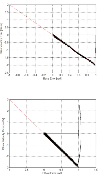
The same behavior can be seen in Figure 4.3 too. The sign function requires infinite switching frequency, in the theory, to keep the system states on the sliding line. However, because of some factors like actuator limitations and delays which are inevitable when the controller is implemented on digital computers, infinite frequency switching cannot be realized. As a result, frequent state trajectory jumps across the sliding line are observed.

Figure 4.3: Sliding mode control without control signal smoothing. Phase plane trajectories for the base and elbow joints. The dashed lines are the sliding surfaces.

27

4.3. Sliding Mode Controller with Modified Controller Gain for Smoothing

This section addresses the smoothing of the control signal and proposes a scheme in

which the controller corrective gains K₁ and K₂ are functions of the absolute values of

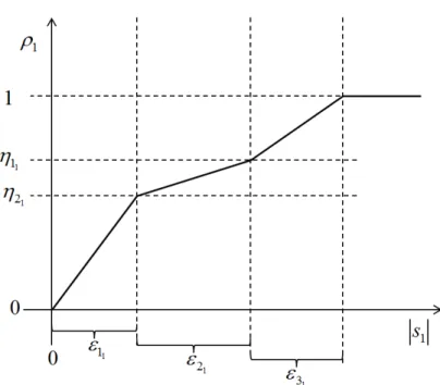
corresponding sliding variables s₁ and s₂. In particular, for example for the base joint, K₁ is modified into the new form

) ( ₁ 1 max 1 K 1 s K = ρ (4.27) where, 1 max

K is a positive constant and ρ₁(s₁) is defined as in Figure 4.3. As seen in this figure,

five parameters, namely,

1 1 ε , 1 2 ε , 1 3 ε , 1 1 η and 1 2

η , define the function

ρ

₁ as a combination of

linear segments (Figure 4.4). The six parameters (

1 max K , 1 1 ε , 1 2 ε , 1 3 ε , 1 1 η , 1 2 η ) defining K₁

provide extensive freedom in tuning. More than or less than three intervals could be used for the

description of the Smoothing Function,

ρ

₁, too. Still, three intervals are rich enough to describe

a curve for control signal smoothing purposes and simple enough for controller tuning.

28

Similarly, the controller gain K₂ is replaced by the expression

) ( ₂ 2 max 2 K 2 s K = ρ , (4.28)

and

ρ

₂ is defined by parameters

2 1 ε , 2 2 ε , 2 3 ε , 2 1 η and 2 2 η . 2 max

K is a positive constant too.

The parameters

j i

ε represent intervals in the s_i axis. It should be noted that

ρ

₁ and

ρ

₂ are restricted to have zero value when their argument is zero. Also they are defined to have unity value at the end of the third interval. The

j i

η parameters are restricted to belong to the closed set

[0,1].

When the absolute value of the sliding variable exceeds beyond the third interval, the control gain becomes a constant, like in the case of the controller derived in the previous section. When the system trajectory comes close to the sliding line (when the sliding variable is small) the value of the control gain is reduced in this scheme, to avoid chattering. As the simulation results below suggest, proper choice of the smoothing parameters above can alleviate the chattering problem.

The simulations are repeated and trial-error based tuning is applied again. The smoothing functions are tuned too. The performances of the controllers are shown in Figures 4.5

and 4.6. The smoothing functions

ρ

₁ and

ρ

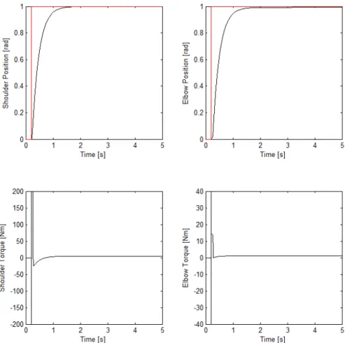
₂ are displayed in Figure 4.7. The values of the

control and smoothing parameters are tabulated in Table 4.2. As can be observed from Figure 4.5, the chattering behavior in the control signal disappeared and the steady state error is small. Figure 4.6 displays the phase plane trajectories. The sliding line is followed after a reaching phase. This behavior is in parallel with exponential (first-order) decay of the errors in Figure 4.5 towards zero.

The experience with the sliding mode controller and smoothing operation described in (4.27) and (4.28) indicate that admissible performance and chattering levels can be attained. However, this work also showed that tuning of the many parameters simultaneously is an elaborate task. This motivates an automatic tuning mechanism. The next chapter handles this problem by the use of GA.

29

Figure 4.5: Sliding mode control with control signal smoothing. Joint positions, step position references and control torques for the base and elbow are shown.

30

Figure 4.6: Sliding mode control with control signal smoothing. Phase plane trajectories for the base and elbow joints. The dashed lines are the sliding surfaces.

31

Figure 4.7: Smoothing functions

ρ

₁ and

ρ

₂ obtained by trial and error and used for the results

presented in Figures 4.5 and 4.6.

Table 4.2

Controller and Control Smoothing Parameters

1 max K 100 Kmax2 50 1

λ

2

λ

₂ 3 1 1 ε 0.2 ε1₂ 0.2 1 2 ε 2 ε2₂ 2 1 3 ε 10 ε3₂ 10 1 1 η 0.4 η1₂ 0.4 1 2 η 0.8 η2₂ 0.8