Florida International University
FIU Digital Commons
FIU Electronic Theses and Dissertations University Graduate School
2-21-2011
Performance Enhancement In Accuracy and
Imaging Time of a Hand-Held Probe-Based
Optical Imager
Sergio L. Martinez
Florida International University, [email protected]
Follow this and additional works at:http://digitalcommons.fiu.edu/etd
This work is brought to you for free and open access by the University Graduate School at FIU Digital Commons. It has been accepted for inclusion in FIU Electronic Theses and Dissertations by an authorized administrator of FIU Digital Commons. For more information, please [email protected]. Recommended Citation
Martinez, Sergio L., "Performance Enhancement In Accuracy and Imaging Time of a Hand-Held Probe-Based Optical Imager" (2011).
FIU Electronic Theses and Dissertations.Paper 397.
FLORIDA INTERNATIONAL UNIVERSITY Miami, Florida
PERFORMANCE ENHANCEMENT IN ACCURACY AND IMAGING TIME OF A HAND-HELD PROBE-BASED OPTICAL IMAGER
A thesis submitted in partial fulfillment of the requirements for the degree of
MASTER OF SCIENCE in
BIOMEDICAL ENGINEERING by
To: Dean Amir Mirmiran
College of Engineering and Computing
This thesis, written by Sergio L. Martinez, and entitled Performance Enhancement in Accuracy and Imaging Time of a Hand-Held Probe-Based Optical Imager, having been approved in respect to style and intellectual content, is referred to you for judgment. We have read this thesis and recommend that it be approved.
_______________________________________ Armando Barreto _______________________________________ Wei-Chiang Lin _______________________________________ Anuradha Godavarty, Major Professor Date of Defense: February 21, 2011
The thesis of Sergio L. Martinez is approved.
_______________________________________ Dean Amir Mirmiran College of Engineering and Computing
_______________________________________ Interim Dean Kevin O’Shea University Graduate School
ABSTRACT OF THE THESIS
PERFORMANCE ENHANCEMENT IN ACCURACY AND IMAGING TIME OF A HAND-HELD PROBE-BASED OPTICAL IMAGER
by
Sergio L. Martinez
Florida International University, 2011 Miami, Florida
Professor Anuradha Godavarty, Major Professor
The Optical Imaging Laboratory has developed a hand-held optical imaging system that is capable of 3D tomographic imaging. However, the imaging system is limited by longer imaging times, and inaccuracy in the positional tracking of the hand-held probe. Hence, the objective is to improve the performance of the imaging system by improving imaging time and positional accuracy. This involves: (i) development of automated single Labview-based software towards near real-time imaging; and (ii) implementation of an alternative positional tracking device (optical) towards improved positional accuracy during imaging. Experimental studies were performed using cubical tissue phantoms (1% Liposyn solution) and 0.45-cc fluorescence target(s) placed under various conditions. The studies demonstrated a 90% reduction in the imaging time (now ~27 sec/image) and also an increase from 94% to 97% in the positional accuracy of the hand-held probe. Performance enhancements in the hand-held optical imaging system have improved its potential towards clinical breast imaging.
TABLE OF CONTENTS CHAPTER PAGE Chapter 1: Introduction ... 1 1.1 Objective ... 2 1.2 Methods... 2 1.3 Hypothesis... 3 1.4 Significance... 3 1.5 Thesis Outline ... 3 Chapter 2: Background ... 5
2.1 Near Infrared Optical Imaging ... 5
2.2 Methods of Optical Imaging ... 6
2.2.1 Sources and Detectors ... 8
2.2.2 Techniques of Optical Imaging ... 9
2.3 Clinical Translation of Optical Imaging ... 11
2.3.1 Hand Held Optical Imagers ... 12
2.4 OIL’s Hand-Held Optical Imager ... 14
2.5 Tracking Devices ... 17
2.6 Co-registration with OIL’s Optical Imager... 21
2.7 Summary ... 23
Chapter 3: Materials and Methods ... 26
Part I Modifications Towards the First Generation Optical Imager ... 26
3.1 Automation of Co-registration ... 26
3.2 Study I: Experimental Evaluation of the Automated Software ... 29
3.3 Study 2: Tracker Evaluation ... 30
3.3.1 Study I: Effectiveness of three trackers towards 2D positioning ... 30
3.3.2 Electromagnetic Tracker Analysis ... 30
3.3.3 Acoustic Tracker Analysis ... 32
3.3.4 Optical Tracker Analysis ... 33
3.4 Optical Tracker Customization ... 33
3.4.1 2D Tracking LED Circuit ... 35
3.4.2 Converting Wiimote Raw Data to Distances ... 36
3.4.3 Operational Limitations of the Wiimote ... 39
3.4.4 Optical Tracker 2D Integration to Automated Software ... 40
3.4.5 2D Co-registration Testing with Tracker ... 43
3.4.6 Optical and Acoustic Tracker 2D Co-registration with Probe ... 44
3.4.7 Fine Movement Tracking with Optical Tracker ... 46
3.5 Customization of Optical Tracker for 3D Tracking ... 46
3.6 Optical Tracker LED Affect on Imaging ... 46
Part II Modifications Towards Second Generation Optical Imager ... 47
3.8 Software Development... 51
3.9 Co-registration ... 53
3.10 2D Co-registration Testing with Tracker ... 57
3.11 2D Tracking ... 58
3.12 2D Co-registered Imaging Testing ... 60
3.13 Summary ... 60
Chapter 4: Results and Discussion ... 62
Part I Modifications Towards the First Generation Optical Imager ... 62
4.1 Study 1: Automated Software ... 62
4.2 Study 2: Tracker Evaluation Results ... 63
4.2.1 Electromagnetic vs. Acoustic Tracking Results ... 63
4.2.2 Optical Tracker Limits ... 65
4.2.3 Optical vs. Acoustic Tracking Results ... 66
4.3 Optical and Acoustic Tracker 2D Co-registration ... 68
4.4 Optical Tracking LED Affect on Imaging ... 72
Part II Modifications Towards Second Generation Optical Imager ... 73
4.5 Second generation Optical Imager ... 73
4.6 Co-registration with the Second Generation Optical Imager ... 77
4.7 2D Tracking with the Second Generation Optical Imager ... 78
4.8 Summary ... 79
Chapter 5: Conclusions and Future Work ... 80
5.1 Conclusion ... 80
5.2 Future Work ... 83
REFERENCES ... 86
LIST OF TABLES
TABLE PAGE
Table 2.1 Comparison of trackers towards tomographic imaging with OIL’s hand held probe shows that optical tracking may provide to be the most
effective………..……...….20 Table 3.1 The comparison of features between first and second-generation optical
imagers..……….49 Table 3.2 Comparison of features of the first and second-generation co-registration
software……….……….…53 Table 3.3 Positions collected in the 2D tracking study for the second generation probe
heads. Both probe heads were moved in the same positions on separate phantoms where (0,0) is the bottom right position of the phantom. Therefore each of these positions was repeated 5 times per probe head.
………....58 Table 4.1 Error comparison of the tracking devices in two dimensional tracking. The
averages of the errors are shown here as well as the average distance from the true measured position as calculated using Equations 3 -
6………...……….…..67 Table 4.2 Comparison of the target location and errors of the probe location for both
trackers. The location of the target was taken from the images that were collected in the 2D studies with a 2% Liposyn filled cubical phantom. The true location of the target was compared to the location found in the images giving the errors shown above.……….71 Table 4.3 Table showing the error of the acoustic, optical, and multiple objects with
optical. Each of the co-registration software’s accuracy was compared in a study where the probe head with the tracker attached was moved along the face of a cubical phantom. The positions at which the probe(s) head was/were located were measured physically and through the co-registration software to provide an accurate comparison of the accuracy of each
LIST OF FIGURES
FIGURE PAGE
Figure 2.1 Time domain signal showing an input signal for tissue imaging. Image
collection is defined as a Temporal Point Spread Function as shown above. ... 9 Figure 2.2 Frequency domain signal showing a sinusoidal input signal for tissue imaging.
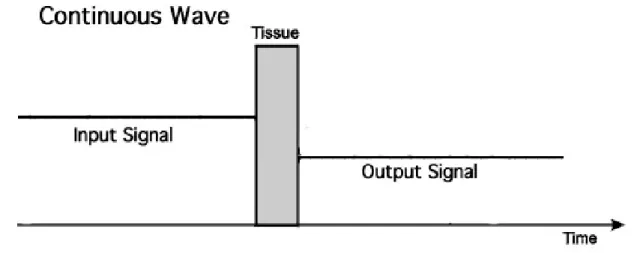
The signal collected also has a sinusoidal shape, however phase shifted. ... 10 Figure 2.3 Continuous wave signal shown is a simple non-modulated source signal for
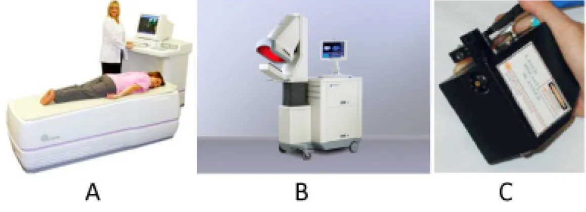
tissue imaging. The detected output light is typically of lower intensity. ... 11 Figure 2.4 Current optical imaging devices. A above is a large bed manufactured by
Imaging Diagnostic Systems, Inc. It involves the breast to be imaged through transillumination while placed in a hole on the imaging bed. B above is also a transillumination imager that requires compression of the breast for imaging [Wang, et al, 2010]. C above is a hand held imager, however is for spectroscopic
measurements [Bevilacqua, et al, 2000]]. ... 12 Figure 2.5 Hand held optical imagers currently in the research stage. A is a round hand
held imager containing 8 sources and a single detector [Chance et al, 2005]. B and C above are both hand held imagers involving optical and acoustic imaging in
combination with one another [Zhu et al, 1999]. ... 13 Figure 2.6 First Generation Hand-Held Probe Head [Jayachandran, et al. 2007] ... 15 Figure 2.7 OIL's hand held optical imager and a blank phantom where (i) is the source,
(ii) is the detector and (iii) is the hand held probe head in contact with a blank
phantom [Jayachandran, et al. 2007] ... 16 Figure 2.8 Acoustic Tracking Device (Logitech tracker manual, Logitech Inc., Fremont,
CA.) ... 18 Figure 2.9 Graphical depiction of the co-registration software's function in (A) obtaining
optical data from WinView and (B) positional data from MatLab simultaneously. The data is then (C) super imposed in LabView to obtain the (D) co-registered image on a mesh of the surface. ... 23 Figure 3.1 Graphical user interface of the new automated software. The focus window on
the right shows the raw image from the camera. Once the “Acquire Image” button is pressed the 2D image collected is displayed. ... 28 Figure 3.2 Flowchart of the software. (A) is where the previous software was run through
Figure 3.3 Polhemus Fastrak Electromagnetic Tracking Device. (A) is the transmitter, (B) is the receiver, and (C) is the control box ... 31 Figure 3.4 Representation of the cubical phantom with the labeled points of where the
tracker receiver was placed ... 32 Figure 3.5 Logitech Ultrasound 3D Head Tracker ... 32 Figure 3.6 Nintendo Wii controllers used as a tracking device where (a) are the Wii
controllers, (b) are the tracked infrared LED’s, and (c) is the Bluetooth waves from the Wii controllers that allow wireless communication with (d) the host computer. 34 Figure 3.7 Flowchart of Wiimote Data Collection Process ... 35 Figure 3.8 LED Circuit ... 36 Figure 3.9 Setup for the 2D tracking equation. The Wiimote was placed at multiple
distances from the (x,y) plane where the LED was placed. The LED was then moved in the x and y direction to determine the equation to convert the pixel values to distances. ... 37 Figure 3.10 Sample of one data set of collected positions to determine the formula to
convert pixels to cm. As can be seen the R2 value average for all samples collected was .99982 with standard deviation of 8.32E-05. The plots show a linear relation between the measured LED position and the pixel value given by the camera. The black line represents the line of best fit. ... 38 Figure 3.11 The angle for field of view was measured using simple geometry. ... 40 Figure 3.12 Flowchart for Wiimote Tracking Integrated into the Co-registration Software
... 42 Figure 3.13 Setup for Tracker and Co-Registration Testing ... 44 Figure 3.14 The figure depicts the motion that was performed on the large 20x20x20 cm
phantom with the probe head and tracker attached to obtain the location of the target in the images collected. A 2% Liposyn phantom and a 1μM indocyanine green (ICG) .45cc target were used. The arrows show the direction of the of the
movements of the probe head . ... 45 Figure 3.15 Depiction of how the effect of the LED on imaging was performed where a
2% Liposyn phantom was used and the LED was placed on the surface of the phantom and on the center of the probe head to see if the IR signal from the LED effects the images collected. ... 47
Figure 3.16 Second Gen Probe Head (left) and the first generation probe head (right). Although the second generation probe heads may be smaller individually, they have more flexibility and are one flexible piece on the probe face allowing for maximum contact while the first generation optical imager is three individual solid plates. .... 48 Figure 3.17 Second generation System in its Cart (left) compared to the first generation
optical imager (right). It can easily be seen that the second-generation system is much more compact and portable than the bench top first generation optical imager. ... 51 Figure 3.18 Second Generation Co-Registration Approach Software Front Panel ... 57 Figure 4.1 Comparison of the results obtained from the electromagnetic tracker and the
acoustic tracker. The transmitter end of each tracker was moved along the four corners of the face of a cubical phantom. ... 65 Figure 4.2 Comparison of tracked positional information using an optical and acoustic
tracker. The LED (optical tracker) and transmitter (ultrasound tracker) were moved in a linear fashion along the face of a cubical phantom. Positions were recorded at .5 cm increments. ... 67 Figure 4.3 Co-registered imaging demonstrating the detection of a target as the probe
head is moved in different positions along the face of a cubical phantom. The black circle represents the position of the.45 cc ICG target within a 2% Liposyn filled cubical phantom. The dotted black box is the outline of the probe head. ... 71 Figure 4.4 2D Contour Images of intensity signals acquired from the phantom surface
under the following conditions: (A) When the LED located on the hand-held probe were turned off, (b) Comparing the effect of the Tracker’s LED On and Off. The LED off image involved the LED being attached to the probe but not powered while the LED on image involved the LED being turned on while attached to the probe. The subtracted image involves the subtraction of the LED on image from the LED off image giving the difference of the two images. ... 73 Figure 4.5 2D surface contour plots of intensity distribution acquired on two 10 x 10 x
10 cc cubical phantoms using the 2 probe heads of the Gen-2 imager. A 0.45 cc absorption contrasted target filled with .08% by volume India Ink was placed in Image collected with the second generation imaging system. The top image displays the images taken with the target in place. The center images display the images taken of the phantom without the target in place. Finally the subtracted images show the lesion location once the background is subtracted from the target. ... 76
Figure 4.6 Co-registered images from the second generation optical imager. The image on the left corresponds to probe 1, and the right to probe 2. Each probe was on a separate cubical phantom and both images were collected with the same camera at the same time. The image is a previously recorded image and does not represent any signal coming from the probe heads or the phantom. ... 77
ACRONYMS
1D One Dimensional
2D Two Dimensional 3D Three Dimensional APD Avalanche Photodiode CCD Charge-Coupled Device
CW Continuous Wave
CT Computed Tomography
DOI Diffuse Optical Imaging EM Electromagnetic
FD Frequency Domain
FDPM Frequency Domain Photon Migration FIU Florida International University GUI Graphical User Interface
ICCD Intensified Charge-Coupled Device ICG Indocyanine Green
LED Light Emitting Diode
MRI Magnetic Resonance Imaging NIR Near-Infrared
OIL Optical Imaging Laboratory
PET Positron Emission Tomography PMT Photon Multiplier Tube
Chapter 1: Introduction
Near-infrared optical imaging is a promising, non-invasive technology with the potential of diagnostic breast imaging. In recent years there has been much research towards the clinical translation of bulky optical imagers, as well as the development of hand held optical imagers. However, current hand-held optical imagers are only capable of two-dimensional (2D) spectroscopic surface images and cannot perform three-dimensional (3D) tomography [Chance, et al. 2005; Chen, et al. 2004; No, et al. 2005; Sao, et a. 2003; Tromberg, et al. 2005; Xu, et al. 2007; Zhu, et al. 1999]. Recently, the Optical Imaging Laboratory (OIL) has developed a hand held optical imaging system that is capable of 3D tomography. To obtain measurements relevant for 3D tomographic imaging, a co-registration technique is employed, that allows registering the positional information of the hand-held probe on the tissue geometry during imaging studies. The feasibility of co-registered imaging and 3D tomography studies on tissue phantoms have been demonstrated in the past. [Ge, et al. 2008; Jayachandran, et al. 2007]. However, there are limitations in our hand-held optical imaging system in the path of our ongoing clinical translational efforts. These include:
(i) Longer imaging times: The optical imaging system and the positional
tracking device are operated independently via their respective software. This is computationally cumbersome and also tends to slow the overall imaging time.
(ii) Instability of the positional tracking device: The ultrasound-based tracking device used to obtain 3D positional information of the hand-held probe during imaging is unstable, thus causing inaccuracies in the 3D positional data. This
in turn tends to impact the location of the detected target during 2D and 3D imaging studies.
1.1 Objective
The objectives of my thesis involve the reduction of the overall imaging times as well as improve the stability and accuracy of the positional tracking device.
1.2 Methods
The methods used to achieve the objective are to:
(i) Develop an automated co-registration technique that can operate both the
optical imaging system and the positional tracking device simultaneously via a single LabView based software. This allows decrease in the overall imaging times as well as makes it user-friendly to perform imaging studies.
(ii) Implement an alternative positional tracking device (optical over ultrasound) and also develop the appropriate software relevant to the tracking device towards automated co-registered imaging. This allows improved stability and accuracy of the positional data during imaging studies, apart from being a cost-effective device.
The automated co-registration software as well as the alternate positional tracking device were developed and implemented into two generations of our optical imaging system.
1.3 Hypothesis
The hypothesis is twofold: (i) Simultaneous operation of multiple tasks during imaging (e.g. image acquisition, positional tracking, and image processing) can significantly reduce the overall imaging time, thus allowing a near real-time imaging in a clinical environment. Additionally, by operating the entire imaging system (including the positional tracking device) using single software, makes the imaging process user-friendly in a clinical setting. (ii) Implementation of an alternate tracking device that is more stable, accurate and cost-effective can improve the accuracy of co-registered imaging, which in turn can improve the quality of target detection.
1.4 Significance
The clinical application of the optical imaging device will complement currently employed imaging tools used towards breast cancer diagnosis. By automating the software, the image acquisition time is decreased to a near real-time imaging approach, which will allow for clinicians to acquire extensive images with least patient time during the diagnostic imaging procedure. By improving the effectiveness of the tracking device, the accuracy in tumor detections can potentially improve, thus preventing invasive methods of locating tumors that are falsely identified.
1.5 Thesis Outline
In chapter 2, the Background of optical imaging and a brief overview of currently available hand-held based optical imagers are described. Additionally, the Optical Imaging Laboratory’s custom built hand held optical imaging system (first generation) is introduced, detailing unique features and shortcomings. Immediately following is a
description of the tracking devices and the concept of co-registration. Chapter 3 is the Materials and Methods of automation of the entire imaging process, and the development and testing of a more accurate and stable tracking device. The development of a second generation hand-held optical imaging system (carried out as a team effort in the laboratory) and the implementation of the developed automated software and the tracking device are also described. Chapter 4 follows with the Results and Discussion of tissue phantom studies that demonstrate near real-time imaging using the automated co-registration software and the alternate positional tracking device. Additionally, the accuracy of the positional tracking device and its effectiveness in 2D target detectability is assessed and compared to the past tracking device. The experimental studies were performed on both the first and second generation hand-held optical imaging systems. Finally, chapter 5 concludes the thesis and summarizes the future direction of the work.
Chapter 2: Background 2.1 Near Infrared Optical Imaging
Breast cancer is the most highly diagnosed cancer in women in the world with an estimated 207,090 new cases in 2010[American Cancer Society, 2010]. Although treating breast cancer is highly important, preventative techniques, such as early diagnosis, are highly valuable in the research community. Current methods of diagnosis include x-ray, x-ray computed tomography (CT), ultrasound, positron emission tomography (PET), and magnetic resonance imaging (MRI). Although for many years these diagnosis techniques have proven to be effective methods of imaging with high sensitivity they suffer from various drawbacks such as
• Radiation from X-Ray and CT can cause harmful effects over
prolonged/multiple uses
• High discomfort used for compressing the breast in X-Ray, CT, and
ultrasound
• Ionization caused by PET can be harmful to the patient
• Poor resolution in ultrasound can make it difficult for doctors and
researchers to determine if and where lesions are present in the tissue
• High cost of MRI causes many people to avoid MRI if they cannot afford
it
• Poor specificity of all these modalities may cause a high number of false positives.
In order to improve on these diagnostic modalities, there is a desire for a less invasive, non-ionizing, high resolution and high specificity/sensitivity imaging technique that is low cost. One technology that has the potential of achieving these objectives is near infrared imaging (NIR).
Near-infrared imaging or optical imaging is a promising invasive, non-ionizing technology for breast cancer diagnosis among countless other uses, such as functional brain mapping and oximetry. NIR uses the therapeutic window of light, 700-900nm wavelength, where light is highly scattered and minimally absorbed in the tissue allowing for tissue characterization through their optical properties. Being minimally absorbed and highly scattered, NIR can also allow for deep tissue imaging giving functional information of biological systems. Although NIR has inherent absorptive properties in tissue, different tissue have different absorptive properties giving an NIR image contrast, which can be further be improved with fluorescing agents to more accurately improve the quality of a collected image using NIR.
2.2 Methods of Optical Imaging
Optical imaging (or NIR imaging), in general, can be performed through many different methods such as spectroscopy and diffuse optical imaging (DOI) among others. Spectroscopic imaging of breast tissue involves the launching of source light into the breast tissue where the reemitted light is then collected by a detector, typically a photodetector, photon multiplier tube (PMT) or avalanche photodiode (APD). Spectroscopy can measure the oxygen content of the hemoglobin in an area of interest thus giving functional information and optical properties of the area through investigation
of the spectra using an inverse algorithm. Diffuse optical imaging refers to the optical imaging of biological tissue in the diffusive regime [Biomedical Optics 2007. DOI systems can be placed in many different source and detector configurations depending on its application for imaging an object, in this case tissue. Image reconstruction in DOT involves both forward and inverse algorithms. In the forward algorithm, the distribution of reemitted light can be predicted based on presumed parameters for the source and object of interest. In the inverse algorithm, the distributions of the optical properties of the object of interest are reconstructed from a measured data set, respectively.
Breast imaging can be performed through configurations including planar transmission or planar reflection [Biomedical Optics 2007]. In general a source will illuminate the area of interest and the detectors will measure the reflected or transmitted light, depending on the configuration. Transmitted light refers to the light that travels through the tissue and is generally collected on the opposite side from where the light is launched. However, transmitted light can also be collected in other areas that are not directly in the same face at which the light was launched into the tissue. Reflected light is that light which is collected on the same face at which the light was launched. Reflectance does not necessarily mean the light hits the surface and reflects back, but it travels through the tissue and scatters in such a manner that it returns to the same face at which the light was launched. Subsequently a computer will take the information collected from the detector and reconstruct the data using complex mathematical techniques. The reconstructed data collected from the tissue will contain a 2D or 3D image mapping the hemoglobin concentrations in the tissue.
2.2.1 Sources and Detectors
In the case of NIR or optical imaging, the wavelengths fall between 700 – 900 nm since light in the tissue is minimally absorbed and preferentially scattered. In order to illuminate the area of interest laser diodes are typically used which emit a particular wavelength of interest. Laser diodes can be placed either in contact with the tissue or illuminate from a particular distance from the tissue producing a more disperse illumination method. Also, in order to transfer the light from one point to another for most systems, optical fibers are used. Although optical fibers can be used to send light from a source laser diode to the tissue, they are also used as a mechanism to transfer light from the tissue surface to the detector. Other methods of illumination include area illuminating white light and LED lighting. With white light the area of interest is illuminated with a halogen or xenon light source, which is usually used in spectral imaging in multiple wavelengths. Optical filters are used on the detector end to collect the wavelengths of interest.
Detectors in optical imaging include photon multiplier tubes (PMT), avalanche photodiodes (APD), and charge coupled devices (CCD). PMTs work in a fashion that multiplies the current produced by incident light in the order of 106, in multiple dynode stages, allowing for individual photons to be detected when the incident light is very low. APDs are a highly sensitive semiconductor electronic device that converts light to electricity by applying a high reverse bias voltage. CCDs work in a fashion where the CCD captures a light signal, which charges the capacitors of the CCD. The charge is then transferred through capacitive bins that manipulate the charge in a manner that converts
order to compensate for the low signal, an image intensifier is used with the CCD thus called an intensified charge coupled device (ICCD).
2.2.2 Techniques of Optical Imaging
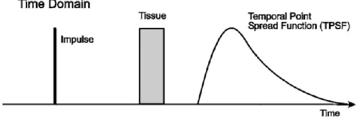
Optical imaging can be classified into three different techniques depending on the type of signal, which are time domain (TD), frequency domain (FD), continuous wave (CW). Time-domain (TD) mode involves a source emitted as an ultra short pulse of light, in the order of picoseconds, into a scattering object as shown in figure 2.1. The reemitted light signal’s response can be resolved through the use of a single photon counting system or streak cameras. The light is collected by a detector such as a CCD, APD, or PMT. Of the three modes, TD contains the most information about the tissue but is also the slowest and most expensive [Wang et al, 2007].
Figure 2.1 Time domain signal showing an input signal for tissue imaging. Image collection is defined as a Temporal Point Spread Function as shown above.
In FD mode, the emitted light source is amplitude modulated and the transmitted/reflected light modulation has a reduced modulation depth as shown in figure 2.2 [Wang et al, 2007]. Typically the output power of a laser diode source is modulated
at a particular frequency from a signal generator and emitted through the tissue. The transmitted/reflected light is collected by the detector, which is modulated as well. Since both source and detector are modulated in frequency domain, the data can be collected via homodyne or heterodyne technique. The homodyne technique is where the source and detector are modulated at the same frequency while the heterodyne technique involves different frequencies for source and detector. The collection of information through FD mode includes amplitude and phase of the signal, which can inherently describe the scattering and absorption coefficients of the tissue through detectors such as PMT, APD, or CCD. FD mode, although contains less information than TD mode, it is much faster and less expensive.
Figure 2.2 Frequency domain signal showing a sinusoidal input signal for tissue imaging. The signal collected also has a sinusoidal shape, however phase shifted.
In CW mode, the source light is time-invariant and contains no direct information about the time of flight of the signal [Wang et al, 2007]. The light is emitted by a laser diode source into the tissue where the reemitted light as shown in figure 2.3, and is then
collected by either a PMT, APD, or CCD. Although the CW mode does not contain no direct information to separate the absorption and scattering, it is the fastest and least expensive of the three modes.
Figure 2.3 Continuous wave signal shown is a simple non-modulated source signal for tissue imaging. The detected output light is typically of lower intensity.
2.3 Clinical Translation of Optical Imaging
Currently, research involving DOI has seen an increase in the clinical translation of this technology using either bulky bench top or hand-held based optical imagers (examples shown in figure 2.4) [Erickson, et al. 2008, Chance, et al. 2005; Chen, et al. 2004; No, et al. 2005; Sao, et a. 2003; Tromberg, et al. 2005; Xu, et al. 2007; Zhu, et al. 1999] for various applications. The larger bench top imagers typically include either a mechanism in which the subject lies face down where the breast is placed in a (semi-spherical) hole containing the source and detector for transmittance configuration of imaging or involving configurations for either transmittance or reflectance configurations with compression applied to the breast. Hand-held imagers are smaller and may or may
not require the application of pressure to the breast, however they have mostly involved in spectroscopic imaging and few tomographic imagers.
Figure 2.4 Current optical imaging devices. A above is a large bed manufactured by Imaging Diagnostic Systems, Inc. It involves the breast to be imaged through transillumination while placed in a hole on the
imaging bed. B above is also a transillumination imager that requires compression of the breast for imaging [Wang, et al, 2010]. C above is a hand held imager, however is for spectroscopic measurements
[Bevilacqua, et al, 2000]]. 2.3.1 Hand Held Optical Imagers
Current hand-held optical imagers (shown in figure 2.5) are primarily able to perform surface scans and provide spectroscopic information, but cannot perform three-dimensional (3D) tomography1 [Chance, et al. 2005; Chen, et al. 2004; No, et al. 2005; Sao, et a. 2003; Tromberg, et al. 2005; Xu, et al. 2007; Zhu, et al. 1999].
Figure 2.5 Hand held optical imagers currently in the research stage. A is a round hand held imager containing 8 sources and a single detector [Chance et al, 2005]. B and C above are both hand held imagers involving optical and acoustic imaging in combination with one another [Zhu et al, 1999].
The type of data that a hand held imager can collect is determined by the configuration of the source and detectors. A single source and detector pair will collect spectroscopic data for simple characterization at a particular point. Tomography usually requires multiple sources and detectors to characterize volumetric information by imaging in sections and then a reconstruction algorithm is used to display a 3D image of the collected slices or images. For these imaging techniques the source and detectors make contact with the breast tissue via a probe head, which is typically the hand held portion of the imager.
Other research groups have based their imaging approach on the photoacoustic methods [Zhu, et al. 1999], which combine ultrasound with the optical data. They obtain the physical information about the tissue as well as the depth aspect of the signal through an ultrasound imaging system while the optical sources and detectors that surround the ultrasound system also collect optical data from the tissue. The optical data is then co-registered with the ultrasound to combine the functional (from the optical data) with the
structural information (from the ultrasound data) and locate a tumor in the tissue [Zhu, et al 2010]. Other groups have developed FD and CW NIR spectroscopic imagers that are capable of collecting both the FD and CW simultaneously allowing for more information about the tissue than just FD or CW alone [Cerussi, et al, 2006; Cerussi, et al, 2007; Erickson, et al 2008], allowing for less post processing to acquire the tissue information. While yet other research groups have also included fluorophores in the tissue or phantoms to enhance the contrast of the image [Erickson, et al 2008].
Although various researchers have developed hand-held probe based imagers with multiple sources and detectors, the probe heads were smaller and the studies were more focused on 2D spectroscopic imaging. Other researchers have yet to successfully combine optical imaging with 3D tomography capabilities in a hand held based system. However in our Optical Imaging Laboratory (OIL), a hand held probe was developed, capable of 3D tomography with multiple sources and detectors placed on a large probe head, towards diagnostic breast imaging studies. OIL is the first to combine simultaneous illumination and detection in a multi-source, multi-detector tomographic hand held imager.
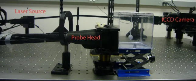
2.4 OIL’s Hand-Held Optical Imager
The hand held optical imager developed in our laboratory (OIL) is based on the homodyne imaging approach. It consists of three major components; (i) the laser diode source (ii) an ICCD detector and (iii) the hand held probe [Ge, et al. 2008; Jayachandran, et al. 2007] as can be seen in figure 2.6. The hand held probe seen in figure 1.6 consists of 165 detector fibers, 6 source fibers and a 3-piece face capable of contouring to curved
surfaces with tissue surface contact. The source fibers are connected to a collimated 785nm laser diode source, while the detector fibers are coupled to the ICCD and focused through a focusing lens. The optical imager is capable of collecting both FD and CW measurements. The source is temperature and current controlled and is coupled to a frequency synthesizer and amplifier for modulation. In order to perform FD optical imaging, the ICCD is also coupled with a frequency synthesizer and amplifier for modulation.
Figure 2.6 First Generation Hand-Held Probe Head [Jayachandran, et al. 2007]
The hand held optical imager has the following unique features:
1. Probe head that can contour to tissue curvatures: Uses a three piece probe face that flexes as seen in figure 2.6 [Jayachandran, et al. 2007].
2. Rapid imaging over large areas: Uses a multi-source illumination
technique with simultaneous detection [Jayachandran, et al. 2007].
3. 3D tomography: Simultaneously tracks 3D positional information and
optical data co-registered onto a mesh of the imaged surface [Ge, et al. 2008; Ge, et al. 2009].
Figure 2.7 OIL's hand held optical imager and a blank phantom where (i) is the source, (ii) is the detector and (iii) is the hand held probe head in contact with a blank phantom [Jayachandran, et al. 2007]
Optical images collected by the optical imager (2D surfaces) are used in appropriate inversion algorithms to obtain 3D image reconstructions. However, 3D image reconstruction is only achieved if the probe’s location is precisely tracked during imaging and superimposed with respect to the imaged surface. The recorded probe head position is acquired using a 3D motion tracker, which is attached to the probe head of the device. The accuracy of the position of a tumor within the tissue can be affected by the accuracy of the tracked position of the hand-held probe during imaging studies. Optical data collected from the camera is superimposed with the tracker data collected from the tracker in a process called co-registration (described in detail in Section 2.6). Therefore, for accurate 3D image reconstructions, an accurate positional tracker is required along with a post-processing tool to co-register for 3D tomography studies. In the following sections the approach of positional tracking and co-registration implemented for the current hand-held optical imaging system are described.
2.5 Tracking Devices
A tracking device is a useful tool towards 3D reconstructions since it allows the probe head’s location to be identified on a computerized mesh of the subject. Tracking devices that use mechanical, inertial, electromagnetic, acoustic, or optical methods can be used to track Optical Imaging Laboratory’s (OIL) probe head [Regalado 2009]. However, mechanical trackers have limited mobility since the object must be affixed to a reference point. Inertial trackers, by nature tend to drift their measurements over time, affecting their accuracy. Therefore mechanical and inertial trackers have not been considered to track the probe head. Since probe head is required to be moved freely in order to obtain multiple images, a positional tracker such as electromagnetic, acoustic, or optical is desired.
Originally an acoustic tracking device from Logitech is in use with the hand held optical probe. The method of tracking used is composed of a transmitter to emit ultrasound waves towards a receiver within its field of view. The receiver has three microphones and is connected to a control box. A transmitter is also connected to the control box and emits the ultrasonic wave towards the receiver. Each microphone on the receiver obtains an acoustic signal that is used to determine its position in space. Figure 3 illustrates the orientation of the acoustic tracker and the setup of its hardware for proper functionality. The acoustic tracker is dependent on a field of view from the transmitter to the receiver, where figure 2.8 illustrates the range of vision as well. Although the acoustic tracker can be accurate, its drawbacks include the lack of flexibility to be customized for a smaller area and instability of the measurements, which can affect the accuracy drastically. The original tracker software was written in C programming
language and its positional data obtained in real-time. However, in order to make the tracker functional with the LabView based co-registration software (see Section 2.6), the data obtained from the tracker was converted via MatLab to positional data appropriate for co-registration. The script converting the raw data to MatLab values causes the tracker to have a lag time (each time that the receiver is moved) of approximately 1 second.
Figure 2.8 Acoustic Tracking Device (Logitech tracker manual, Logitech Inc., Fremont, CA.)
To improve upon the current method of tracking’s instability, two other types of tracking methods will be analyzed, electromagnetic and optical. Table 2.1 describes the advantages and disadvantages of each of the trackers, which is described in more detail. Electromagnetic (EM) trackers are well known to be used in various applications (Raab, et al. 1979; Roetenberg, et al. 2007), are accurate, and do not require large hardware for tracking. The EM tracker uses orthogonal coils on the receiver and transmitter to determine the magnetic field vector of the coils. The relative magnetic field of the receiver and the transmitter determines the position and orientation of the receiver. They are very fast and very accurate even when obstructed by a large object since they do not
require a field of view. However, if metallic objects are present near the magnetic field of the tracker, the data is greatly affected.
Optical trackers operate very similar to the acoustic tracker since they require a field of view in order to track the object and vary in prices depending on the components necessary. The optical tracker can be very fast and very accurate depending on the detector used (Meeks, et al. 2005; Reed 2002). The electromagnetic, acoustic, and optical trackers will be assessed for accuracy of tracking to improve the accuracy of the co-registration (see Chapter 3).
Advantages Disadvantages
Table 2.1 Comparison of trackers towards tomographic imaging with OIL’s hand held probe shows that optical tracking may provide to be the most effective.
2.6 Co-registration with OIL’s Optical Imager
Co-registration is the method by which the collected image is super imposed with metallic objects or magnetic fields sight between transmitter and receiver • Expensive • Cannot be customized • Unstable
• Lag time of 1-2 sec
Electromagnetic Tracking • No line of sight is necessary • Can be wireless • Relatively Fast • Expensive • Affected by metallic objects and magnetic fields
Optical Tracking • Low cost
• Easily customized
• Wireless
• Fast and Stable
• Requires line of sight between detector and source
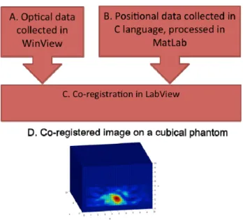
the positional data and then projected onto a computerized representation of the imaged surface [Regalado, et al. 2009]. To obtain a 3D reconstruction of a 2D image collected via an optical imager, the collected image must be superimposed with the positional data with respect to the imaged surface. The custom developed co-registration software (written in LabView) acquires the data collected from the optical imager (using WinView software) and superimposes it onto the tracker’s positional data (obtained using MatLab) in order to obtain a co-registered image. Figure 2.9 illustrates the combination of the various software outputs to obtain a single co-registered image. The optical images acquired via Winview are initially saved and further uploaded into the LabView based co-registration software, making it a time consuming process. On the other hand, the tracked positional information in Matlab is an in-built part of the co-registration software, with least lag time (~ 1 sec). This multi-software based co-registration approach causes the entire process of obtaining a co-registered image as long as 5 minutes each time. When multiple images need to be acquired and co-registered towards 3D tomographic imaging, the entire imaging process might take minutes to hours. Hence, there is a need to enhance the efficiency of the co-registration software by reducing the overall image acquisition time.
Figure 2.9 Graphical depiction of the co-registration software's function in (A) obtaining optical data from WinView and (B) positional data from MatLab simultaneously. The data is then (C) super imposed in
LabView to obtain the (D) co-registered image on a mesh of the surface. 2.7 Summary
In summary, the combination of the unique features of the developed optical imager (described in Section 2.4) has provided a novel method of 3D optical tomography via the use of a hand held probe head. Although all these features are unique and have provided the ability to perform 3D tomography, the hand held optical imager experiences the following shortcomings:
1. Lack of full contact with tissue: The three plate design of the probe head has sharp edges that do not make contact with the tissue.
2. Uneven source distribution: The six sources are collimated from a single laser where there is an uneven intensity distribution among the six sources. This uneven source distribution is difficult to account for in image reconstruction.
3. Multiple software co-registration: Multiple software causes the imaging processing to be longer, thus increasing the overall imaging time in a clinical set-up.
4. Unstable positional tracking: Instability arising from the tracker affects the accuracy of the reconstructions through error in the positioning of the collected images.
The potential solutions to these shortcomings have led to the development of the next generation imager. These solutions include:
1. A more flexible probe head with smooth (and no sharp) edges to contour with maximum contact onto different tissue curvatures (part of another student’s research in the laboratory).
2. An alternate instrumentation at the source end such that it provides
uniform intensity of multiple simultaneous sources (part of another student’s research in the laboratory).
3. A modified co-registration software that is fully-automated and also
minimizes the overall co-registration time (my thesis focus).
4. An alternate tracking device with improved stability and accuracy, at a lower cost and smaller size (my thesis focus).
Herein, my research goals are primarily focused:
Specific Aim 1: To reduce the imaging time during co-registration by minimizing the amount of manual input necessary for the software to
achieve a shorter time of completion, an automated software will be developed that will perform all the functions performed separately by Winview, MatLab and LabView.
Specific Aim 2: To improve the accuracy of the co-registered imaging via the use of efficient tracking devices. Electromagnetic, acoustic, and optical trackers will be assessed and compared. The comparison of the three trackers will determine the best fit for the optical imager.
My research goals will be primarily focused with improving the first generation imager. Once the first generation imager has shown improvement, the work completed will be implemented towards the second generation optical imager.
Chapter 3: Materials and Methods
The multi-software co-registration approach used in the first generation optical imager [Ge, et al. 2008; Ge, et al. 2009] will be converted to an automated software package. As the co-registration software is automated with a new software approach, the time of imaging will improve. However, improving the time for imaging will not suffice unless the accuracy and stability of positional tracking are improved. By comparing multiple tracking approaches, a more accurate and stable device can be selected to improve the overall accuracy of co-registration. The following chapter describes (i) the methods of automating and improving the co-registration process and (ii) the method of improving the tracking accuracy for the first and second generation optical imagers. Part I Modifications Towards the First Generation Optical Imager
3.1 Automation of Co-registration
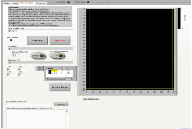
The original co-registration software for the imager involved a multi-software (MatLab, WinView, and LabView) co-registration approach to achieve a co-registered image as described in Section 2.5. A complete automation of the co-registration and image collection process was ideal for reducing the time of co-registration. By automating the image acquisition process with the positional data acquisition and co-registration, the amount of time to collect and co-register one image can be reduced. A simple graphical user interface (GUI) was created along with the automation to minimize user input. Figure 3.1 below is the part of the GUI where the images are collected. A simple click of a button acquires the image and then can be co-registered in another part of the GUI. Figure 3.2 below shows the flowchart for the process of the automated
co-registration software. The area labeled in A within the dotted box was originally the WinView based detector control and image acquisition software. The part labeled B, outside of the dotted box in the flowchart is the area which was created in LabView for the co-registration of the collected images. The flowchart describes the sequence of steps performed by the co-registration software. First the camera is initialized and focused, before an image is acquired (Steps 1-3). Parallely, the position of the hand-held probe is tracked using the tracker in 3D (Steps 6-7). Step 8 in the flowchart is the mathematical operation that correlates (superimposes) the positional data (Step 7) and the acquired image (Step 3) in order to position the 2D image on the (simulated) computerized probe. A post-processing subtraction technique is employed to account for background noise in the optical images during the image acquisition process (Step 9). This step is optional and used as needed during imaging studies. Prior to imaging studies, a discretized mesh of the tissue phantom being imaged is generated (Step 4) and uploaded into the co-registration software (Step 5). The correlated (and post-processed) optical images and positional data (from Step 9) are co-registered onto the 3D discretized tissue phantom mesh (Step 10) using the uploaded mesh (Step 5). The co-registered images are displayed (Step 11) and further stored (Step 12), such that the software is ready for acquiring the next set of images in near-real time until the experiment is complete (Step 13).
Figure 3.1 Graphical user interface of the new automated software. The focus window on the right shows the raw image from the camera. Once the “Acquire Image” button is pressed the 2D image collected is
Figure 3.2 Flowchart of the software. (A) is where the previous software was run through WinView and has now been integrated with (B) the LabView based co-registration software for full automation.
3.2 Study I: Experimental Evaluation of the Automated Software
The automated software was tested for comparison of the time of one image collection with the multi-software approach. Comparison of imaging time was performed during phantom studies where image data collection was done using continuous wave measurements from tissue phantoms. For both software the same computer was used which has a dual core (virtual quad core) Intel 3.2 GHz processor and 4GB of RAM on Windows XP (32-Bit).
3.3 Study 2: Tracker Evaluation
Currently an ultrasound tracker is used with the hand held optical imager. However, it has been observed throughout our experiments that there is a significant amount of instability during the tracking process. A fluctuation of about +/- .5 cm about the true position of the tracker has been observed. In order to reduce error, a more stable tracker is desired. Therefore, two different trackers were assessed, which include electromagnetic and optical trackers. For each tracking device, similar methods of accuracy testing were performed and will be described in the following Sections.
3.3.1 Study I: Effectiveness of three trackers towards 2D positioning
The effectiveness of the three tracking devices in accurate positional information in real-time was assessed via a comparison study. The effectiveness of the three trackers was assessed from 2D studies wherein the receiver or source end of the trackers was moved along the four corners of a phantom and the horizontal and vertical positional information was collected (keeping the depth constant). The measured positions and true physical positions were compared to determine the most effective tracker towards improvement of the co-registration for 2D co-registered imaging with the hand-held probe.
3.3.2 Electromagnetic Tracker Analysis
The study involved the evaluation of the electromagnetic tracker (Polhemus FasTrak, Polhemus, Colchester, VT) in comparison to the acoustic and optical trackers. The Polhemus Fastrak utilizes a wired setup where the receiver and transmitter are connected to a control box as shown in figure 3.3. Polhemus provides a stand-alone
software to collect positional data from the EM tracker. To test the tracker, the receiver was placed on a single face of a blank cubical phantom. The square face of the phantom measures 8.5 cm x 8.5 cm and the receiver end of the tracker was placed at each of the corners of the face (seen in figure 3.4) and measured physically as well as using the software. The accuracy of the tracker was determined by comparing the physically measured position of the receiver with the given position form the software. To test the accuracy of the magnetic tracker in true experimental situations, the tracker was also attached to the first generation hand held probe, which contains metal, in order to observe the effect that the metal has on its positional data.
Figure 3.3 Polhemus Fastrak Electromagnetic Tracking Device. (A) is the transmitter, (B) is the receiver, and (C) is the control box
Figure 3.4 Representation of the cubical phantom with the labeled points of where the tracker receiver was placed
3.3.3 Acoustic Tracker Analysis
The study also involved an evaluation of the acoustic tracker (Logitech 3D Head Tracker in figure 3.5) for comparison with the EM and optical tracking devices. The method of assessing the tracker’s accuracy was similar to the EM tracker where the receiver was placed at each of the corners of a single face of a blank cubical phantom and measured physically as well as through the software. The accuracy was compared through individual point collection and continuous data streaming, which was obtained for the determination of stability while moving the receiver, as well as leaving the receiver at rest.
3.3.4 Optical Tracker Analysis
The optical tracker (which will be discussed in section 3.4) was a customized Nintendo Wii Remote and was compared the EM and acoustic tracker. The method of assessing the tracker’s accuracy was similar to the EM tracker where the receiver was placed at each of the corners of a single face of a blank cubical phantom and and measured physically as well as through the software. The accuracy was compared through individual point collection, which was measured physically as well as through the custom software. Continuous data streaming was also obtained for the determination of stability while moving the LEDs, as well as leaving the LEDs at rest.
3.4 Optical Tracker Customization
The optical tracker chosen for the current study was a very inexpensive tracker originally used as a controller for a video game console. A Nintendo Wii Remote, or also called the Nintendo Wiimote (see figure 3.6), was used as the optical tracker with an AZiO micro Bluetooth Adapter for the computer connection. The Nintendo Wiimote contains an infrared camera with a 1024X768 pixel resolution with built-in post processing allowing for four LEDs to be tracked at a time.
Figure 3.6 Nintendo Wii controllers used as a tracking device where (a) are the Wii controllers, (b) are the tracked infrared LED’s, and (c) is the Bluetooth waves from the Wii controllers that allow wireless
communication with (d) the host computer.
In order for the tracker to be used with a computer, a connection must be made through Bluetooth and a custom code written to use its tracking capabilities. There are very few Bluetooth software, or Bluetooth stacks, which can appropriately control the amount of information coming from the Wiimote as a tracking device. Therefore BlueSoleil was used to handle the Bluetooth communication between the computer and the Wiimote. The figure below shows the flowchart of the Wiimote tracking process.
Figure 3.7 Flowchart of Wiimote Data Collection Process 3.4.1 2D Tracking LED Circuit
The Nintendo Wiimote originally uses (infrared) LEDs for the Nintendo Wii’s software to determine the position and movements of a user. Therefore, to use the Wiimote as a tracking device on a computer an infrared source array was developed to use as the object to be tracked. Infrared LEDs operating at 940 nm wavelength with a 100 mA forward current were used. Each circuit required 2 LEDs, three 1 Ohm resistors per LED, and a 1.5 V AA battery as per Ohm’s Law. The two LED’s were placed in parallel in order to supply enough current to them from a single battery. Figure 3.8 below illustrates the circuit used. Since the LED array is the object to be tracked by the Wiimote, any object attached to the LED array will also be tracked.
Figure 3.8 LED Circuit 3.4.2 Converting Wiimote Raw Data to Distances
The Wiimote was customized as required for the development of 2D tracking software since it was not inherently a tracking device. Tracking information acquired from the Wiimote is represented directly as raw data, where each given value by the Wiimote corresponds to a particular pixel value on the camera of the Wiimote. Therefore an experimentally derived equation was determined such that each pixel of the camera would correspond to a particular distance traveled in horizontal and vertical directions dependant on the distance the source was from the camera. To determine the equation for the conversion of the pixel value given by the camera to distance travelled by the LEDs, the Wiimote was placed at a fixed location and the source LEDs were moved. The LEDs were placed at 5 experimentally varied depths and 10 lateral/vertical positions at each depth, where each position was physically measured as shown in figure 3.9. Once the pixel value for each position and at each distance was given, equation 1 was determined through curve fitting. A sample data set collected at 30 cm depth is shown, where the formulae given are the best-fit line of the data collected. In order to achieve the actual slope of the line necessary for conversion as in equation 1, the slope of each line and for each data set was divided by the distance from which it was collected. An average was
then taken for the slope of each data set and used as the conversion factor in equation 1. In order to test the accuracy of the determined equation, 30 known and measured positions were taken and the (Nx,Ny) values given by the Wiimote were compared to the
measured positions.
Figure 3.9 Setup for the 2D tracking equation. The Wiimote was placed at multiple distances from the (x,y) plane where the LED was placed. The LED was then moved in the x and y direction to determine the
Figure 3.10 Sample of one data set of collected positions to determine the formula to convert pixels to cm. As can be seen the R2 value average for all samples collected was .99982 with standard deviation of
8.32E-05. The plots show a linear relation between the measured LED position and the pixel value given by the camera. The black line represents the line of best fit.
Equation 1
The variable d in equation 1 represents the measured distance in centimeters that the source (i.e. LED) is from the detector (i.e. Wiimote), (Px,Py) is the respective horizontal
and vertical pixel value given by the detector (Wiimote), and finally (Nx,Ny) is the actual
position of the source (LED) in centimeters. At each distance, a line of best fit was determined for the data collected, where the distance measured for the position of the pixel was a function of the pixel value given by the Wiimote (as shown in Figure 3.10). Each data set had a plot similar to Figure 3.10 with the line of best fit given by the equation of a line, y=mx + b. In order to determine the slope of the conversion equation (equation 1), the slope of each line was divided by the distance (between the Wiimote and
y = 0.0232x - 14.944 R² = 0.9997 y = 0.0243x - 8.095 R² = 0.9998 -12 -10 -8 -6 -4 -2 0 2 4 6 8 10 0 500 1000 1500 Measured Di stance (cm)
Pixel Value Given by Camera (px)
Curve Fitting at 30 cm distance
X direction Movement Y direction Movement Linear (X direction Movement) Linear (Y direction Movement)
N
x,
N
y(
)
=
(
.000783
×
d
)
•
(
P
x,
P
y)
LED) for each data set and then averaged. The value .000783 was determined to be the average slope (or the conversion factor) by the above formulation, with a standard deviation of 1.79E-05. The constant ‘b’ in this linear equation, y=mx+b, was not given in equation 1, since it is given by what pixel value the user determines to be zero, and will be described in 3.4.4 (which is related to the calibration of the tracker). By using equation 1, the 2D location of the LEDs can be obtained as the LEDs are moved in real time, as long as the distance from the x-y plane (where the LEDs are located) to the Wiimote is known (i.e. d in equation 1).
3.4.3 Operational Limitations of the Wiimote
Once equation 1 was verified, the limitations of operation of the Wiimote were determined. Knowing the operating limits of the Wiimote, experimental setups can then be determined so that the LEDs are always in view of the Wiimote, preventing errors due to exiting the field of view or detection limits of the Wiimote. The maximum distance of detection of the LEDs was determined by moving the LEDs away from the Wiimote until the LEDs were not visible to the Wiimote, where the distance was found to be 173 cm. Also, the maximal field of view was determined by fixing the Wiimote on an elevated surface and moving the IR LEDs known distances up, down, left, and right to detect the full field of view of the camera where the measured field of view was determined through simple geometry. Since the distance of the LED to the Wiimote was known, and the height of the LED was known, the angle at which the LED was from the Wiimote (θ) was determined as depicted in figure 3.11 and using equation 2. The maximum field of view angle of the Wiimote was found to be 43°.
Figure 3.11 The angle for field of view was measured using simple geometry. θ =tan−1 y x Equation 2
3.4.4 Optical Tracker 2D Integration to Automated Software
In order to be able to perform the co-registration in an experimentally comparable method, the software developed for 2D tracking was integrated into the automated software. The acoustic tracker files were removed from the software preventing the software from attempting to communicate with a non-existent tracker. Once the files were removed, the files created for communication with the tracker were integrated in place of the acoustic tracker’s files. The formula was directly encoded into the LabView software to quickly perform the calculations. MatLab was then used for the conversion of the Wiimote data in equation 1 and the output numbers for the LED location were used as inputs for the m-files that perform the co-registration mathematics. An input was added to the front panel of the software for the distance at which the LEDs are from the Wiimote, allowing for the calculation of the 2D position of the LEDs attached to the probe head. All the tracker data is collected and converted in real time to allow for the most accurate and fastest data collection possible.
Figure 3.12 below describes the flow of the co-registration process used in the developed software. The co-registration begins by loading the 3D mesh of the phantom into the software and the communication with one or more Wiimotes is initiated. Communication with the Wiimote’s allows for the real time acquisition of data from the Wiimote, which is converted to useful distance measurements through a MatLab script involving equation 1. The MatLab script is integrated to the Labview software to allow for automatic transfer of data through the software for real time tracking of the probe heads. In figure 3.12, the boxed area identifies the portion modified from the original ultrasound based registration software to the new optical tracking based co-registration software. The acquired images are co-registered onto the imaged surface by using the 2D positional information. Finally the image is saved and the process is repeated for each collected co-registered image.
Figure 3.12 Flowchart for Wiimote Tracking Integrated into the Co-registration Software
Although the tracking system accurately converts pixel data to positional values, a reference point can be used in order to have a zero point and track all positions in relation to that reference point. Initially starting the tracker at a reference point will display an arbitrary value for the position of the LED. However, this initial position is the reference point, which requires a value of (0,0). In order to reinitialize the system to zero at the reference point and determine all other positions in relation to the reference point, a method of re-initialization was developed. Subtraction of the initial position from every position given by the tracker allows the real positions and distances traveled to be displayed in relation to the reference point (0,0) as given by Equation 3.
in cm Equation 3
In equation 3, (Cx,Cy) is the new reinitialized position given by subtracting the initial (N0,N0) position of the tracker and the current (Nx,Ny) position from the tracker. (N0,N0) can now be considered the ‘b’ (or y-intercept) of the line equation, y=mx+b, as described in Section 3.4.2.
3.4.5 2D Co-registration Testing with Tracker
Implementation of the tracker was the first step of integration towards the first generation imager. Once the software was ready to be tested, the circuit developed for 2D tracking was used on an aluminum block to view the accuracy that the co-registration had of imaging (using a dummy image). A false image was loaded into the co-registration software, and a mesh of the cubical phantom was used. The aluminum block to be tracked was initialized at the bottom right of the cubical phantom and the false image was co-registered in position. The aluminum block was then moved in a manner mimicking the probe head’s movements during a phantom study. The Wiimote was placed a distance of 25, 35, and 45 cm from the LEDs and the aluminum block was moved to 20 different (x,y) positions for each distance on a 20cm × 20cm × 20cm cubical phantom. The accuracy of the tracker was determined, while testing the functionality of the co-registration software. Figure 3.13 below shows the set up of the study that was performed to determine the accuracy of the optical tracker during co-registration of a previously recorded image without the use of the probe heads. The phantom was annotated (using tape in two axes) to easily read the measured positions on the face of the phantom on which the LED source were to be placed and to compare the results given
C
x,
C
yfrom the computer to those measured positions. The co-registered images were saved and the values given by the co-registration software regarding the positions were compared to the physically measured values.
Figure 3.13 Setup for Tracker and Co-Registration Testing 3.4.6 Optical and Acoustic Tracker 2D Co-registration with Probe
The optical and acoustic trackers were compared in their ability to track the probe head as well as their impact on the position of the target in a phantom. As explained in section 3.3, the position of the receiver corresponds to the position of the probe head. The receiver of the acoustic tracker and the LED’s of the optical tracker were placed on the probe head and used with the co-registration software during phantom studies. A large cubical phantom (20cm × 20cm × 20cm) was filled with 2% Liposyn solution. A target with 1μM indocyanine green (ICG) of size 0.45cc was placed in the phantom at 1
cm depth, 5.5 cm vertically, and 9 cm horizontally as figure 3.14 depicts. The probe head was placed directly in contact with the face of the phantom and images were collected at heights of 1, 2, and 3 cm vertically and 4, 5, and 6 cm horizontally for a total of 9 images for acoustic and optical tracker based hand-held probe. At these multiple positions the target is visible in the images collected and the positions can be compared to the physical position of the probe head. In addition to 2D and 3D location of the probe head, the images collected are also used to determine the effect the tracking device has on locating the position of the target. The target is in a known location and the images that are collected will provide the coordinates for which the target is found on the probe face.
Figure 3.14 The figure depicts the motion that was performed on the large 20x20x20 cm phantom with the probe head and tracker attached to obtain the location of the target in the images collected. A 2% Liposyn phantom and a 1μM indocyanine green (ICG) .45cc target were used. The arrows show the direction of the

![Figure 2.5 Hand held optical imagers currently in the research stage. A is a round hand held imager containing 8 sources and a single detector [Chance et al, 2005]](https://thumb-us.123doks.com/thumbv2/123dok_us/1869481.2772790/25.918.293.744.106.321/figure-optical-imagers-currently-research-containing-sources-detector.webp)