Time Series Forecasting with Missing Values
Shin-Fu Wu, Chia-Yung Chang, and Shie-Jue Lee
Department of Electrical Engineering
National Sun Yat-Sen University
Kaohsiung 80424, Taiwan
{sfwu,cychang}@water.ee.nsysu.edu.tw, [email protected]
Abstract—Time series prediction has become more popular in various kinds of applications such as weather prediction, control engineering, financial analysis, industrial monitoring, etc. To deal with real-world problems, we are often faced with missing values in the data due to sensor malfunctions or human errors. Traditionally, the missing values are simply omitted or replaced by means of imputation methods. However, omitting those missing values may cause temporal discontinuity. Imputation methods, on the other hand, may alter the original time series. In this study, we propose a novel forecasting method based on least squares support vector machine (LSSVM). We employ the input patterns with the temporal information which is defined as local time index (LTI). Time series data as well as local time indexes are fed to LSSVM for doing forecasting without imputation. We compare the forecasting performance of our method with other imputation methods. Experimental results show that the proposed method is promising and is worth further investigations.
Keywords—Time series prediction, missing values,local time index, least squares support vector machine (LSSVM)
I. INTRODUCTION
In general, a time series can be defined as a series of observations taken successively every equally spaced time interval. The primary goal of time series prediction is to forecast the future trend of the data based on the historical records. Therefore, it plays an important role in the decision making for industrial monitoring, business metrics, electrical grid control and various kinds of applications. We can roughly categorize the time series problems as follows. If we want to forecast one time step ahead into the future, which is the most case of time series problems, it is called a one-step or single-step prediction. On the other hand, if we make a prediction that is multiple time step ahead into the future, it is called a multi-step prediction. There are two approaches to make a multi-multi-step prediction, direct and iterative. The direct approach is to build a model that forecasts multi-step ahead results directly while the iterative approach is to make multiple one-step predictions iteratively until it reaches the required step.
Recently, artificial intelligence is gaining popularity in the time series prediction. Support vector machine (SVM) is one of the most popular tools for time series prediction using artificial intelligence. The major development of SVM was done by Vapnik and his colleagues in the AT&T Bell Laboratories in the 1970s. It was initially set for classification problems and real-world applications such as optical character recognition. In [1], support vector machine was extended to solve regression problems. Support vector machine is free from local minimum from which neural networks suffer. However, the computa-tional burden of solving quadratic programming problems is
quite heavy. Least squares support vector machine (LSSVM) was introduced in [2] which transfers the constraint problems into a linear system. The LSSVM reduces the computational costs but the sparsity of the support vectors is lost. The weighed LSSVM was proposed [3] to offer an alternative solution to the sparsity problem. In recent years, LSSVM is adopted in different fields of applications, especially the time series prediction and financial forecasting.
In many real-world cases, we are faced with missing values in time series data. These missing values occurs due to sensor malfunctions or human errors. Various ad hoc techniques have been used to deal with missing values [4]. They include deletion methods or techniques that attempt to fill in each missing value with one single substitute. The ad hoc techniques may result in biased estimations or incorrect standard errors [5]. However, they are still very common in published re-searches [6][7][8]. Multiple imputation [9][10] and maximum likelihood [11] are two recommended modern missing data im-putation techniques. Multiple imim-putation creates several copies of original missing data and each of the copies is imputed separately. Analyzing each copy yields multiple parameter estimates and standard errors and they will be combined into one final result. On the other hand, maximum likelihood uses all the available data to generate estimates with the highest probability. Multiple imputation and maximum likelihood tend to produce similar results and choosing between them is sort of personal preference.
Performing time series prediction with missing data is a dif-ficult task. The temporal significance in time series prediction makes it different from other forms of data analysis. Ignoring those missing values destroys the continuity of a time series. Replacing the missing values with imputation methods alters the original time series and it may severely affect the prediction performance. It is hard to evaluate how the predicted results are affected by forecasting models or imputation methods. In this paper, we develop an approach to solve the prediction problems based on the structure of LSSVM. A series of local time indexes are introduced before the training phase of LSSVM. Time series data as well as local time indexes are fed to LSSVM for doing forecasting without imputation. This paper is organized as follows. In Section II, we give a general idea of the time series data with missing values and what we want to predict. In Section III, we describe how LSSVM works in Section III-A and detail the local time index (LTI) approach in Section III-B. In Section IV, we compare our methods with other imputation techniques on several time series datasets. In Section V, we summarize the results of our study and show the directions of future works.
INISCom 2015, March 02-04, Tokyo, Japan Copyright © 2015 ICST
II. PROBLEMSTATEMENT
LetSi¯ ={xi,¯ yi¯}, where1≤i≤m is the time index, be a series of multivariate data taken every equally spaced time interval∆t. That is,S¯1was taken att1,S¯2was taken att1+∆t,
. . . , and the final observationSm¯ was taken att1+ (m−1)∆t.
In a simple multivariate case, each observation contains two variables x¯ andy¯wherex¯ is the additional variable and y¯ is the desired output. On the contrary, each observation contains only one variabley¯in a univariate case. In this paper, we only consider the case with two variables as follows:
¯
xi = {xi,xi˙ }, (1)
¯
yi = {yi,y˙i} (2)
wherei= 1, . . . , mand
{
xi=null, xi˙ = 0 ifxi¯ is missing ; xi= ¯x, x˙i= 1 otherwise (3)
{
yi=null, yi˙ = 0 ifyi¯ is missing; yi= ¯y, y˙i= 1 otherwise (4)
Note that xandy are available data, and x˙ andy˙ denote the flags of available values. Ifx¯andy¯contains no missing values, our goal is to find the function f such that
ˆ
yt+q−1+s=f(xt, yt, xt+1, yt+1, . . . , xt+q−1, yt+q−1) (5)
where (xt, yt, xt+1, yt+1, . . . , xt+q−1, yt+q−1) is called the
input query, q is the query size, t is the time index, ands is step size. Ifs= 1in Eq. 5,f is called a single-step or one-step forecasting model. If s >1 in Eq. 5, f is called a multi-step forecasting model. The direct approach predicts ytˆ+q−1+s di-rectly from (xt, yt, xt+1, yt+1, . . . , xt+q−1, yt+q−1) while the
iterative approach is to predict ytˆ+q and then ytˆ+q+1,ytˆ+q+2,
. . . ,ytˆ+q−1+siteratively.
III. PROPOSEDMETHOD
In this section we describe how least squares support vector machine (LSSVM) is applied to time series prediction with missing values. The basic idea is “Local Time Index” (LTI) which ignores the missing values and adopts additional temporal information into the training patterns.
In the case with no missing values, we can formulate the training patterns P from Eq. 5 for the LSSVM as follows:
Pt = {Qt, Tt} (6)
Qt = (xt, yt, xt+1, yt+1, ..., xt+q−1, yt+q−1) (7)
Tt = yt+q−1+s (8)
whereqis the query size,t is the time index from1 toM = m−q−s+ 1, andsis the step size. Therefore,mobservations generateM training patterns.
A. Least Squares Support Vector Machine
Given a set of time series patternsPt={Qt, Tt}in Eq. 6. Our goal is to find the estimated function shown as follows:
ˆ
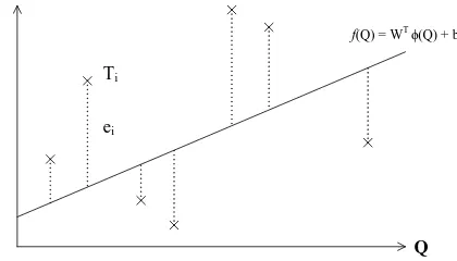
T =f(Q) =WTϕ(Q) +b (9)
We want tot minimize the error between T and Tˆ and keep W as small as possible. A large value of W will make this
model sensitive to the perturbations in the features which is not favourable. Therefore, the objective function can be written as
min 1 2∥W∥
2
+C 2
M
∑
i=1
e2i (10)
subject toTi=WTϕ(Qi) +b+ei (11) fori= 1, ..., M
whereei is the error andC is the regulation parameter which determines the rigorousness of this model. A large number of C allows a small error while a small number of C allows a large error in Eq. 10. An illustration of LSSVM is shown in Figure 1. We reformulate the objective function and constraints
Q
Ti
ei
f(Q) = WT ϕ(Q) + b
Figure 1. An illustration of LSSVM for time series prediction.
in Eq. 10 and Eq. 11 into Lagrangian formulation. There are two reasons for doing the Lagrangian formulation [12]. The first one is that constraints in Eq. 11 will be replaced by the constraints on the Lagrange multiplier themselves which are easier to handle. The second one is this reformulation will keep the input patterns in the dot products between vectors. There-fore, we introduce Lagrange multipliersαiwherei= 1, ..., M, one for each constraint in Eq. 11. The constraint equations are multiplied by the Lagrange multipliers and subtracted from the objective function. This gives the following Lagrangian:
Lp(W, b, e, α) =
1 2∥W∥
2
+C 2
M
∑
i=1
e2i + M
∑
i=1
αi(Ti−WTϕ(Qi)−b−ei)
(12)
Our goal is to minimize Eq. 12. The Lagrange multiplier αi can be either positive or negative due to the equality constraints of Karush-Kuhn-Tucker conditions [13][14]. By making derivatives ofLp vanish, we have the conditions for optimality:
∂Lp
∂W =W − M
∑
i=1
αiϕ(Qi) = 0
∂Lp ∂b =−
M
∑
i=1
αi= 0
∂Lp
∂ei =Cei−αi= 0 ∂Lp
∂αi =Ti−W
Tϕ(Qi)−b−ei= 0
These conditions can be written as the solution to the following set of linear equations:
[
K+CI 1M 1TM 0
] [
Λ b
]
=
[
Γ 0
]
(14)
where K is a M-by-M kernel matrix, kij = k(Qi, Qj) = ϕT(Qi)ϕ(Qj), Γ = [T
1 T2 ... TM]T, Λ = [α1 α2 ... αM]T
and 1M = [1 1 ... 1]T is a vector with M 1’s. After calculating the Λ and b in Eq. 14, the estimated function
ˆ Tj =
M
∑
i=1
αik(Qi, Qj) +b can be found. Therefore, we can make a prediction ofTj from the given input queryQj.
B. Local Time Index
Due to the introduction of missing values, we can not formulate the training patterns as Eq. 6 without any imputation. However, we do not want to manipulate the time series data which may cause more problems due to the performance of imputation methods. Ignoring the missing vales is the simplest idea but doing this will break the continuity of the time series. If we provide temporal information to those patterns with missing values, the forecasting model can somehow extract the temporal significance of certain time series data. This is the intuition of our method. From Eq. 1 and Eq. 2, we have m observed variables¯xandy:¯
¯
x = {x,x˙}, (15)
¯
y = {y,y˙} (16)
wherexandy may contain null elements due to missing val-ues. We ignore those missing values and extract the available sets of values from xandy. The available set can be written as follows:
Ax = {A1x, A
2
x, ..., A u x},
tx = {t1x, t2x, ..., tux} (17) Ay = {A1y, A2y, ..., Avy},
ty = {t1y, t2y, ..., tvy} (18)
where x has u available elements in total, Au
x is the uth available element inxand the corresponding global time index is tu
x, tux > txu−1 > ... > t1x. Similarly, y has v available elements in total, Av
y is thevthavailable element iny and the corresponding global time index is tv
y,tvy> tvy−1> ... > t1y. We can now formulate the training patterns from the available sets in Eq. 17 and Eq. 18. We take the formulation of theithtraining pattern for s-step prediction as an example. Firstly, we set thejth= (v−i+ 1)th element (Ajy) inAy as the training target, Ti. Secondly, we fetch the q elements in Ay as the inputs from variabley¯and we have to maintain the time indexes of those elements smaller than tj
y −s+ 1. For the additional variablex, we fetch the last¯ q elements and we also have to make sure that time indexes should be smaller than tj
y−s+ 1. After all the input elements are fetched, input query Qi is done and we can obtain a sequence of corresponding global time indexes GT Ii (with the target time index). We define the local time indexesLi as
tmin = min(GT Ii),
Li = GT Ii−tmin (19)
Finally, theith generated pattern can be written as
Pi={{Qi, Li}, Ti} (20) After all the patterns are generated, we normalize L to the range [0,1] by the maximum local time index. The detailed algorithm of local time index is described in Algorithm 1. This algorithm can be extended to more than one additional variable easily.
Algorithm 1 The algorithm of local time index with 2
vari-ablesx¯ andy¯
Construct Ax fromx;¯ Construct Ay from y;¯ i= 1;
END = false;
while END == falsedo
Qi→ϕ,Ti→ϕ;
j =v−i+ 1{fetch query fory¯}; l=u−i+ 2 {fetch query forx¯}; Set thejth element inA
y as the training targetTi;
fork= 1→q do
ydone = false;
while ydone == falsedo
if tj−k
y <(tjy−s+ 1) then Qi←(j−k)th element inAy; ydone = true;
else
j=j−1; ydone = false;
end if;
end while;
xdone = false;
while xdone == falsedo
if tl−k
x <(tjy−s+ 1) then Qi←(l−k)th element inAx; xdone = true;
else
l=l−1; xdone = false;
end if;
end while;
end for;{Qi is done!}
{Check stopping criterion!}
if size ofQi<2q then
END = true;
else
Retrieve GT Ii and calculateLi; Pi={{Qi, Li}, Ti};
end if;
i=i+ 1;
end while;
IV. EXPERIMENTALRESULTS
the closest observation to the missing value as the candidate. AR imputation is proposed in [15] and it uses auto-regression model (p = 4) to fill in missing values. They are tested on 3 generated datasets (sine function, sinc function, and Mackey-Glass chaotic time series) and 4 benchmark datasets (Poland electricity load, Sunspot, Jenkins-Box, and EUNITE competition). The experiments are performed in the following manner:
• Create a time series of data with R% missing rate at random.
• Training Phase:
1) Reconstruct the training time series using a imputation method (by mean, hot-deck and AR imputation).
2) Train the LSSVM prediction model with the reconstructed series.
3) For LTI, we generate the training patterns using Algorithm 1 and send them to LSSVM.
• Testing Phase:
1) Construct the testing query using a imputation method if it contains missing values.
2) For LTI, we generate the testing query in the same way as in the training phase.
3) Feed the testing query into the trained model and calculate the result.
The performance of each method is measured by the normal-ized root mean squared error (NRMSE) defined below:
NRMSE =
√∑Nt
i=1(yi−yˆi)2 Nt
ymax−ymin , (21) whereNtis the number of testing data,yi is the actual output value andyiˆ is the estimated output value, fori= 1,2, . . . , Nt. Note that ymax and ymin are the maximum and minimum, respectively, ofyi in the whole dataset. The following experi-ments are implemented in Matlab R2012b and executed on a computer with AMD PhenomTMII X4 965 Processor 3.4 GHz and 8 GB RAM.
A. Sine Function
The time series data of the Sine function is generated by the following equation:
y=sin(t) (22)
where t ∈ [−10,10) and the time interval of t is 0.02 and we generate 1000 time series samples. The first 500 samples are for training and the other 500 samples are for testing. The query sizeqis 4, step sizesis 1, and the parameters of LSSVM are determined in the training phase and they are not changed during the testing phase. The NRMSE and time consumption of each method are shown in Table I. From this table, we can see that LTI offers comparable or even better NRMSE values. Furthermore, LTI runs much faster.
Table I. COMPARISON ONNRMSEAND TIME ONSINE FUNCTION
R mean hot-deck AR LTI
5% 0.0513 0.0024 0.0069 0.0021 10% 0.0743 0.0037 0.0094 0.0030 15% 0.0979 0.0050 0.0151 0.0042 20% 0.1171 0.0063 0.0357 0.0050 25% 0.1275 0.0071 0.0358 0.0053 50% 0.3145 0.0155 0.1156 0.0124 time (sec) 7.6230 5.2508 26.1742 1.7851
B. Sinc Function
The time series data of the Sinc function is generated by the following equation.
y=
{ sin(t)
t , ift̸= 0; 1, ift= 0
(23)
where t ∈ [−10,10) and the time interval of t is 0.02 and we generate 1000 time series samples. The first 500 samples are for training and the other 500 samples are for testing. The query size q is 4, step size s is 1, and the parameters of LSSVM are determined in the training phase and they are not changed during the testing phase. The NRMSE and time consumption of each method are shown in Table II. Again,
Table II. COMPARISON ONNRMSEAND TIME ONSINCFUNCTION
R mean hot-deck AR LTI
5% 0.0579 0.0132 0.0165 0.0112 10% 0.0537 0.0191 0.0239 0.0101 15% 0.0950 0.0109 0.0108 0.0073 20% 0.1061 0.0176 0.0226 0.0153 25% 0.1156 0.0188 0.0209 0.0094 50% 0.1065 0.0286 0.0373 0.0283 time (sec) 5.1152 4.8754 27.3818 1.7188
we can see that LTI offers comparable or even better NRMSE values. Furthermore, LTI runs much faster.
C. Mackey-Glass Chaotic Time Series
The well-known Mackey-Glass time series [16] is gener-ated by the following equation:
dy(t) dt =
0.2y(t−τ)
1 +y10(t−τ)−0.1y(t) (24)
where τ = 17, the initial condition y(0) = 1.2, and the time step ∆t = 1. The data is sampled every 6 points and we generate 1000 data points. The first 500 samples are for training and the other 500 samples are for testing. The query size q is 4, step size s is 1 and the parameters of LSSVM are determined in the training phase and they are not changed during the testing phase. The NRMSE and time consumption of each method are shown in Table III. For this experiment, LTI offers better NRMSE values in particular whenR is low to moderate. Still, LTI runs faster than the other methods.
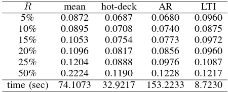
D. Poland Electricity Load
Table III. COMPARISON ONNRMSEAND TIME ONMACKEY-GLASS CHAOTICTIMESERIES DATASET
R mean hot-deck AR LTI
5% 0.1166 0.0975 0.1016 0.0806 10% 0.1137 0.0968 0.0994 0.0825 15% 0.1333 0.1096 0.1314 0.1215 20% 0.1493 0.1157 0.1401 0.1126 25% 0.1597 0.1279 0.1551 0.1407 50% 0.2494 0.2166 0.2672 0.2080 time (sec) 6.8915 5.4388 27.1048 1.8945
1,000 observations for training and the next 500 observations for testing. The query size q is 9, step size s is 1, and the parameters of LSSVM are determined in the training phase and they are not changed during the testing phase. The NRMSE and time consumption of each method are shown in Table IV. For this experiment, LTI runs much faster than the other
Table IV. COMPARISON ONNRMSEAND TIME ONPOLAND ELECTRICITYLOAD DATASET
R mean hot-deck AR LTI
5% 0.0872 0.0687 0.0680 0.0960 10% 0.0895 0.0708 0.0740 0.0875 15% 0.1053 0.0754 0.0773 0.0972 20% 0.1096 0.0817 0.0856 0.0960 25% 0.1204 0.0888 0.0976 0.1087 50% 0.2224 0.1190 0.1228 0.1217 time (sec) 74.1073 32.9217 153.2233 8.7230
methods.
E. Sunspot
This dataset [18] is a univariate time series data set which records the yearly sunspot number from year 1700. The data from year 1700 to 1920 are used for training and the data from year 1920 to 1987 are used for testing. The query size q is 10, step size s is 1, and the parameters of LSSVM are determined in the training phase and they are not changed during the testing phase. The NRMSE and time consumption of each method are shown in Table V. As can be seen, LTI
Table V. COMPARISON ONNRMSEAND TIME ONSUNSPOT DATASET
R mean hot-deck AR LTI 5% 0.1383 0.1310 0.1294 0.1235 10% 0.1561 0.1485 0.1545 0.1345 15% 0.1572 0.1325 0.1547 0.1443 20% 0.1882 0.1702 0.1795 0.1518 25% 0.1862 0.1568 0.1597 0.1408 50% 0.2731 0.1778 0.2217 0.2278 time (sec) 1.2732 1.0918 1.8899 0.6014
not only offer good estimations but also runs faster than the other methods.
F. Jenkins-Box Gas Furnace
This dataset [19] is a multivariate time series data set [20]. It consists of 296 pairs of examples {ai, bi} where ai is the input gas rate and bi is the CO2 concentration from the gas
furnace. We use these two variables to predict future CO2
concentration. The data with time index from 1 to 250 are used for training and those from 251 to 296 are used for testing. The query size q is 6, step size s is 1, and the parameters of LSSVM are determined in the training phase and they are not changed during the testing phase. The NRMSE and time consumption of each method are shown in Table VI. Again,
Table VI. COMPARISON ONNRMSEAND TIME ONJENKINS-BOXGAS FURNACE DATASET
R mean hot-deck AR LTI 5% 0.1015 0.0639 0.1722 0.0583 10% 0.0999 0.0628 0.1578 0.0556 15% 0.1164 0.0673 0.1636 0.0589 20% 0.1054 0.0831 0.1663 0.0709 25% 0.1177 0.0896 0.1544 0.0621 50% 0.1586 0.1010 0.1828 0.1162 time (sec) 1.2422 1.2225 2.2252 0.5116
for this dataset, LTI not only offer better estimations but also runs faster than the other methods.
V. CONCLUSION
We have presented a novel method to make prediction for time series data with missing values. We introduce the local time index to the training and testing patterns without using any kind of imputation as other methods do. When making prediction using LSSVM, the kernel function measures not only the values between two patterns, but also the temporal information we provide. The general performance of our proposed method is good and the time complexity is low as well. However, as other methods, over-fitting can be an issue with our method. There are some directions for the future research in this topic. One is to solve the over-fitting problem by applying fuzzy logic on the local time index. Another one is to provide extra weights to the LSSVM model based on the temporal information.
REFERENCES
[1] H. Drucker, C. J. C. Burges, L. Kaufman, A. J. Smola, and V. N. Vapnik, Support Vector Regression Machines, Advances in Neural Information Processing Systems 9, NIPS 1996, pp. 155-161, MIT Press.
[2] J. A. K. Suykens, T. Van Gestel, J. De Brabanter, B. De Moor, and J. Vandewalle, Least Squares Support Vector Machines, World Scientific Pub. Co., Singapore, 2002.
[3] J. A. K. Suykens, J. De Brabanter, L. Lukas, and J. Vandewalle, Weighted least squares support vector machines: robustness and sparse approximation, Neurocomputing, vol. 48, pp. 85-105, 2002.
[4] A. N. Baraldi and C. K. Enders, An introduction to modern missing data analysis, Journal of School Psychology, vol. 48, pp. 5-37, 2010. [5] R. J. A. Little and D. B. Rubin,Statistical Analysis with Missing Data,
2nd Ed., Hoboken, NJ: Wiley, 2002.
[6] J. L. Peugh and C. K. Enders,Missing data in educational research: A review of reporting practices and suggestions for improvement, Review of Educational Research, vol. 74, pp. 525-556, 2004.
[7] T. E. Bodner, Missing data: Prevalence and reporting practices, Psychological Reports, vol. 99, pp. 675-680, 2006.
[8] A. M. Wood, I. R. White, and S. G. Thompson, Are missing outcome data adequately handled? A review of published randomized controlled trials in major medical journals, Clinical Trials Review, vol. 1, pp. 368-376, 2004.
[10] D. B. Rubin, Multiple imputation after 18+ years, Journal of the American Statistical Association, vol 91, no. 434, pp. 473-489, 1996. [11] P. D. Allison, Missing Data, Thousand Oaks, CA: Sage Publications,
2001.
[12] C. J.C. Burges, A tutorial on support vector machines for pattern recognition, Data Mining and Knowledge Discovery, vol. 2, pp. 121-167, 1998.
[13] R. Fletcher, Practical Methods of Optimization, 2nd Ed., John Wiley and Sons, Inc., 1987.
[14] J. A. K. Suykens and J. Vandewalle, Least squares support vector machine classifiers, Neural Processing Letters, vol. 9, pp. 293-300, 1999.
[15] S. Stridevi, D. S. Rajaram, C. SibiArasan, and C. Swadhikar, Impu-tation for the analysis of missing values and prediction of time series data, IEEE-International Conference on Recent Trends in Information Technology, 2011.
[16] M. Mackey and L. Glass,Osillation and chaos in physiological control systems, Science, vol. 197, pp. 287-289, 2008.
[17] Poland Electricity Load Dataset website: http://research.ics.aalto.fi/eiml/datasets.html [18] Sunspot Dataset website:
http://sidc.oma.be/sunspot-data
[19] Jenkins-Box Gas Furnace Dataset website: http://www.stat.wisc.edu/ reinsel/bjr-data/