Data visualization of item-total correlation by median smoothing

(1)

Practical Assessment, Research, and Evaluation

Volume 21 Volume 21, 2016 Article 1

2016

Data visualization of item-total correlation by median smoothing

Chong Ho Yu Samantha Douglas Anna Lee

Min An

Follow this and additional works at: https://scholarworks.umass.edu/pare Recommended Citation

Recommended Citation

Yu, Chong Ho; Douglas, Samantha; Lee, Anna; and An, Min (2016) "Data visualization of item-total correlation by median smoothing," Practical Assessment, Research, and Evaluation: Vol. 21 , Article 1. DOI: https://doi.org/10.7275/3bwx-7134

Available at: https://scholarworks.umass.edu/pare/vol21/iss1/1

This Article is brought to you for free and open access by ScholarWorks@UMass Amherst. It has been accepted for inclusion in Practical Assessment, Research, and Evaluation by an authorized editor of ScholarWorks@UMass Amherst. For more information, please contact scholarworks@library.umass.edu.

(2)

Copyright is retained by the first or sole author, who grants right of first publication to is granted to distribute this article for nonprofit, educational

right to authorize third party reproduction of this article in print, electronic and database forms. Volume 21, Number 1, February 2016

Data V

isualizati

by

Chong Ho Yu, Min An,

This paper aims to illustrate how data visualization could be modeling, using an example with multi

item response theory and factor analysis to identify a psychometric model that investigates two or more latent traits. While it may seem convenient to accomplish two tasks by employing one procedure, users should be cautious of problematic items that affect both factor analysis and IRT. When sample sizes are extremely large, reliability analyses can misidentify even random number meaningful patterns. Data visualization, such as median smoothing, can be used to identify problematic items in preliminary data cleaning.

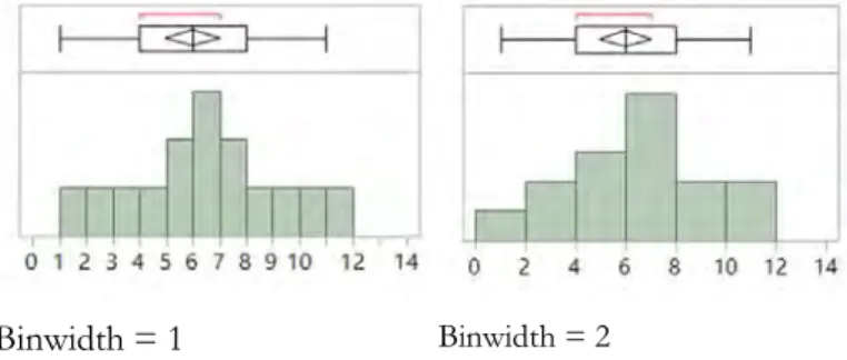
Data visualization is an indispensable tool for pattern recognition in data analysis (Cleveland, 1993; Few, 2009; Tufe, 1990, 1997, 2001 2006; Yu & Stockford, 2003; Yu, 2014). While some data visualization techniques display both raw data and smoothed structure (e.g. regression line) simultaneously, some aim to reduce data noise by smoothing only (summarizing data). Smoothing is prevalent in many data visualization techniques though users may not be aware of it. Take the histogram as an example. While requesting a histogram from any statistical software package seems to be straightforward, the appearance of the histogram is tied to the interval width, also known as the binwidth. Usually a statistical package does not show all data values with numerous bars. Rather, it groups values into several intervals (bins). When a wider binwidth is used, the histogram appears to be smoother. One of the problems of histogram binning is that the choice of binwidth is arbitrary. As a result, the same data set might appear differently in different histograms. For example, in Figure 1 the distribution of the histogram appears to be normal when the binwidth is set to one, but it turns to a skew distribution when the binwidth is

A peer-reviewed electronic journal.

Copyright is retained by the first or sole author, who grants right of first publication to Practical Assessment, Research & Evaluation.

is granted to distribute this article for nonprofit, educational purposes if it is copied in its entirety and the journal is credited. PARE has the right to authorize third party reproduction of this article in print, electronic and database forms.

isualizati

on of Item-Total C

orrelation

by

Median Smoothing

Chong Ho Yu, Samantha Douglas, Anna Lee, Azusa Pacific University

Min An, LinyiUniversity; Hong Kong Institute of Education

This paper aims to illustrate how data visualization could be utilized to identify errors prior to modeling, using an example with multi-dimensional item response theory (MIRT). MIRT combines item response theory and factor analysis to identify a psychometric model that investigates two or t may seem convenient to accomplish two tasks by employing one procedure, users should be cautious of problematic items that affect both factor analysis and IRT. When sample sizes are extremely large, reliability analyses can misidentify even random number meaningful patterns. Data visualization, such as median smoothing, can be used to identify problematic items in preliminary data cleaning.

spensable tool for pattern recognition in data analysis (Cleveland, 1993; Few, 2009; Tufe, 1990, 1997, 2001 2006; Yu & Stockford, 2003; Yu, 2014). While some data visualization techniques display both raw data and smoothed structure (e.g. regression line) simultaneously, some aim to reduce data noise by smoothing only (summarizing data). Smoothing is prevalent in many data visualization techniques though users may not be aware of it. Take the histogram as an example. While requesting a histogram from any atistical software package seems to be straightforward, the appearance of the histogram is tied to the interval width, also known as the binwidth. Usually a statistical package does not show all data values with numerous bars. Rather, it groups values several intervals (bins). When a wider binwidth is used, the histogram appears to be smoother. One of the problems of histogram binning is that the choice of . As a result, the same data set erent histograms. For example, in Figure 1 the distribution of the histogram appears to be normal when the binwidth is set to one, but it turns to a skew distribution when the binwidth is

changed to two. Nonetheless, the boxplo

histograms show that the distribution is indeed symmetrical. This simple illustration shows that data interpretation can be misconstrued when an analyst is not aware of the arbitrariness of smoothing preference.

Binwidth = 1 Binwidth = 2

Figure 1. Two histograms depicting the same data set with different binwidths.

Bubble Plot

Histograms depict only one

however, when the data set is bivariate or multi dimensional, smoothing becomes more complicated and difficult. When the sample size is very large, the dots in a bivariate scatterplot forms a big “cloud.” One way to simplify this over-plotted graph is the binning Practical Assessment, Research & Evaluation. Permission purposes if it is copied in its entirety and the journal is credited. PARE has the ISSN 1531-7714

orrelation

Azusa Pacific University

utilized to identify errors prior to dimensional item response theory (MIRT). MIRT combines item response theory and factor analysis to identify a psychometric model that investigates two or t may seem convenient to accomplish two tasks by employing one procedure, users should be cautious of problematic items that affect both factor analysis and IRT. When sample sizes are extremely large, reliability analyses can misidentify even random numbers as meaningful patterns. Data visualization, such as median smoothing, can be used to identify

changed to two. Nonetheless, the boxplots above both w that the distribution is indeed symmetrical. This simple illustration shows that data interpretation can be misconstrued when an analyst is not aware of the arbitrariness of smoothing preference.

Binwidth = 2

depicting the same data set with

Histograms depict only one-dimensional data; however, when the data set is bivariate or multi -dimensional, smoothing becomes more complicated and difficult. When the sample size is very large, the dots in a bivariate scatterplot forms a big “cloud.” One plotted graph is the binning

(3)

Practical Assessment, Research & Evaluation, Vol 21, No 1

Yu, Douglas, Lee, & An, Data Visualization

approach (Carr, 1991), which follows and extends the

same logic of grouping bars in a histogram. The difference is that in a bivariate plot data points are grouped in bivariate intervals and larger symb indicating more data points. This approach, which is known as the bubble plot, is available in several software packages, such as Mathematica (Wolfram, 2013) and JMP (SAS Institute, 2015) (See Figure 2). Specifically, when data are dense in a particula

of the scatterplot, the bubble becomes bigger. Conversely, when the data are sparse, the bubble is smaller. One shortcoming of the bubble plot approach is that the scale of the bubble is arbitrary. For example, in one plot a circle with an area of 1cm

represent 10 observations but in another it might symbolize 100.

Figure 2. Bubble plot. Density Contour Plot

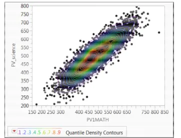
Another way to overcome over-plotting is the density contour plot. In this approach the density of data points is represented by both colors and contour lines. As shown in Figure 3, the large amount of data that concentrate on the centroid are depicted by colored contours. One advantage of this method is that noisy data are not hidden. Rather, the contours are superimposed on top of the raw data. However, this type of depiction is not intuitive and even a well

data analyst may not be able to discover the pattern or the trend in the data set. The obstacle is that if the

Vol 21, No 1

Visualization

approach (Carr, 1991), which follows and extends the

same logic of grouping bars in a histogram. The difference is that in a bivariate plot data points are grouped in bivariate intervals and larger symbols indicating more data points. This approach, which is known as the bubble plot, is available in several software packages, such as Mathematica (Wolfram, 2013) and JMP (SAS Institute, 2015) (See Figure 2). Specifically, when data are dense in a particular location of the scatterplot, the bubble becomes bigger. Conversely, when the data are sparse, the bubble is smaller. One shortcoming of the bubble plot approach is that the scale of the bubble is arbitrary. For example, of 1cm2_might

represent 10 observations but in another it might

plotting is the density contour plot. In this approach the density of data points is represented by both colors and contour lines. As shown in Figure 3, the large amount of data that concentrate on the centroid are depicted by colored contours. One advantage of this method is that noisy data are not hidden. Rather, the contours are superimposed on top of the raw data. However, this type of depiction is not intuitive and even a well-trained r the pattern or the trend in the data set. The obstacle is that if the

contour lines are not portrayed with additional labels, it is not informative at all (Boyd, 2015).

Figure 3. Density contour plot. Sunflower Plot

The sunflower plot is another

to over-plotting (Cleveland & McGill, 1984). In a sunflower plot, the density of the data points is symbolized by a glyph. The more observations the spot contains, the more rays it emanates from the center. If there are more observations in a particular location, the glyph would look like a “sunflower” (see Figure 4). However, Schilling, and Watkins (1994) explained that when there is only one observation in a spot, the symbol is just a dot rather than a sunflower. As a result, it is difficult to synthesize both dots and sunflowers into a coherent image. In addition, mentally translating the rays into frequency increases the cognitive load. Further, when there are two observations only, a single line extends from that point. It may mislead the analyst to perceive that only one observation is there.

Figure 4. Sunflower plot.

Page 2

contour lines are not portrayed with additional labels, it is not informative at all (Boyd, 2015).

unflower plot is another proposed solution plotting (Cleveland & McGill, 1984). In a sunflower plot, the density of the data points is symbolized by a glyph. The more observations the spot contains, the more rays it emanates from the center. If in a particular location, the glyph would look like a “sunflower” (see Figure 4). and Watkins (1994) explained that when there is only one observation in a spot, the symbol is just a dot rather than a sunflower. As a fficult to synthesize both dots and sunflowers into a coherent image. In addition, mentally translating the rays into frequency increases the cognitive load. Further, when there are two observations only, a single line extends from that point. ead the analyst to perceive that only one

(4)

Practical Assessment, Research & Evaluation, Vol 21, No 1 Page 3 Yu, Douglas, Lee, & An, Data Visualization

Another way to simplify an over-plotted

scattergram is median or mean smoothing. In this approach when the software algorithm encounters too many data, it can divide the data into several partitions along the x–axis and then calculate the median of y in each segment (Tukey, 1977). Hence, the analyst can look at the trend by visually connecting the medians. Mihalisin, Timlin, and Schwegler (1991) extended the preceding idea by using the mean rather than the median. However, using the median is recommended because the median is more resistant against extreme scores, especially when the distribution of a certain slice of the data set is highly skewed. It is the conviction of the authors that the median smoothing approach is more effective than all of the preceding methods. The meaning of median (middle point) is universally accepted while the scale of the bubble or the interval of contour lines is subject to the analyst’s preference. Hence, the pattern or the trend unveiled by median smoothing has a more objective ground. This will be demonstrated next.

Methodology

In this paper data visualization by median smoothing is illustrated by an example in item response theory (IRT), which is a powerful psychometric tool that is capable of estimating item attributes and person traits without the restriction of sample-dependence (Embretson & Reise, 2000). IRT assumes unidimensionality, meaning that a test or a survey used with these approaches should examine only a single latent trait of participants. In reality, many tests or surveys are multi-dimensional. If unidimensionality assumption is not satisfied, researchers can choose to remove unfit items, or to identify internal structure by conducting some exploratory factor analysis and confirmatory factor analysis. Then items belonging to different constructs can be scaled separately. However, critics charge that psychometric properties such as factor loadings are sample-dependent (Embretson & Reise, 2000; Wright & Mok, 2000), and thus structure produced from one study may be so unstable that it varies from sample to sample (Yan & Mok, 2012). To address these issues, multi-dimensional IRT (MIRT) was introduced as a synthesis of factor analysis and IRT (Adams, Wilson, & Wang, 1997; Kamata & Bauer, 2008). It performs well when sub-scales within an instrument are strongly correlated with each other (Wang, Yao, Tsai, Wang, & Hsieh, 2006).

MIRT aims to model latent covariance structures between multiple dimensions, and also to model these interactions (Hartig & Hohler, 2009). A classic example involves latent traits required for solving a math problem. When a math problem is presented in a formula or an equation (e.g. Solve y = 2x + 5; 2y = x + 10), the required problem-solving ability is mathematical skill alone. However, if a math problem is explained in text (e.g. A car is running 65 miles per hour and the distance between the starting point and the destination is 485 miles. How long does it take for the car to reach the destination?), both math and reading skills are required.

Several software packages are capable of running MIRT; these include Mplus, ITPRO, flexMIRT, EQSIRT, and SAS (SAS Institute, 2014). At first glance it is efficient to accomplish two tasks (identification of the factor structure and the item characteristics) concurrently. However, it is important to recognize that if problematic items are present in the data set, neither factor modeling nor IRT modeling can be successfully performed. This problem is especially severe when sample sizes are extremely large. Both factor analysis and IRT are very demanding in sample size. The recommended minimum sample sizes for factor analysis range from 150 to 500 (Comrey & Lee, 1992; Hutcheson & Sofroniou, 1999; MacCallum, Widaman, Preacher, & Hong, 1999; Mundfrom, Shaw, & Ke, 2005). For IRT, suggested minimum sample sizes could be as large as 1,000 or 2,000 (Baker, 1992; Hulin, Lissak, & Drasgow, 1982). With such large sample sizes, calibrations and estimations may not be very accurate. At the same time, problematic items may be hidden in the large data set.

There are many ways to detect and remove problematic items. In classical test theory, a typical approach is to examine the point-biserial correlation (item-total correlation) of each item. In IRT or Rasch modeling, it is common to examine discrimination parameters (Nikolausa et al., 2013) and infit or outfit Chi-square, in order to detect bad items (Lai, Cella, Chang, Bode, & Heinemann, 2003; Yu, 2013). This paper illustrates another way of identifying poor items - namely, data visualization of item-total correlation by median smoothing.

Data Source

As mentioned before, problematic items might be buried by an extremely large sample. To make the

(5)

illustration as realistic as possible, a large archival data

set was downloaded from the website, “Personality Tests” (http://personality-testing.info/). Specifically, data collected using the Consideration of Future Consequences Scale (CFCS) was chosen. The objective of CFCS is to measure to what extent individuals take potential future outcomes into account while doing things at the present time and to what extent their current behaviors are influenced by imagined outcomes. There were five possible answers on the CFCS: extremely uncharacteristic (1), somewhat uncharacteristic (2), uncertain (3), somewhat characteristic (4), and extremely characteristic (5). Higher scores indicated a greater level of consideration of future consequences. Originally the CFCS was developed as a one-dimensional scale (Strathman, Gleicher, Boninger, & Edwards, 1994). However, recent factor analyses suggested that this scale carries two dimensions: consideration of the immediate and consideration of the future (Heveya et al., 2010; Joireman, Balliet, Sprott, Spangenberg, & Schultz, 2008; Joireman, Shaffer, Balliet, & Strathman, 2012; Joireman, Strathman, & Balliet, 2006). The original sample size of the full data set was 15,035. Two hundred and sixteen observations were removed, due to erroneous data or missing values. As a result, the remaining number of observations was 14,819.

The original CFCS has 12 items and the revised version has 14. This data set is based on the original scale but in order to illustrate the importance of preliminary item selection the authors added two problematic items into the data set. As mentioned before, when sample sizes are too large, even random numbers may appear to form a pattern. Hence, if there are problematic items in the data set, they may not be detected. To demonstrate this problem, random number generating functions were used to insert two items (Q13 and Q14) into the scale. In Q13 the same probability (.2) was assigned to the five answer categories (1= extremely uncharacteristic, 2= somewhat uncharacteristic, 3= uncertain, 4= somewhat characteristic, 5= extremely characteristic). Therefore, this item had a uniform distribution. In Q14 a higher probability (.4) was assigned to the middle category (3), whereas lower probabilities were assigned to the other categories. Specifically, Category 2 and 4 have a probability of .2 to appear whereas Category 1 and 4 have a probability of .1. As a result, a normal distribution was created.

The uniform distribution of item Q13 was generated to mimic how the factors of ‘fatigue’ and ‘boredom’ affect data accuracy. If a survey is too long or participants perceive its items as irrelevant, participants might randomly select one of the five categories, rather than reading the questions carefully. These respondents might not choose the same answers (e.g. all ‘A’s or all ‘B’s) throughout the survey, in order to avoid detection of their feigned or mindless responses. As a result, each category would have an equal chance of being selected.

The normal distribution of item Q14 was generated in order to simulate problems with poorly worded and/or misfit items. Even if an item is intended to fit into a construct under study, a poorly worded item may confuse and mislead participants. For example, in a survey pertaining to the attitude towards science learning the following question could be asked: “Do you think that fundamental physics is difficult?” Fundamental physics is a study of the basic structure and universal properties of nature, such as particles and quantum fields. While some respondents may interpret this question correctly, some might think that it refers to elementary physics. Consequently, its response pattern might still be a normal curve, but it would be disconnected from all other items. In the case of a misfit item there would be no vagueness in the wording, but the item would not be strongly related to the construct under investigation. For example, in a survey about mental wellbeing the following question could be asked: “Do you consider yourself physically healthy?” Responses to this question would not indicate a significant association between happiness and physical health. In this case the responses would still be normally distributed but the item would be misfit to the focal construct.

Results

Exploratory Factor Analysis The original data set yielded a high Cronbach’s Alpha (.8717); no item(s) needed to be excluded in order to substantively improve the scale’s reliability. In other words, the response pattern to all of the questions was internally consistent (see Figure 5).

(6)

Figure 5. Cronbach’s alpha of the original 12 items.

Concurring with the literature, exploratory factor analysis (EFA) suggested a 2-factor solution based on the scree plot (see Figure 6) and the factor structure depicted in the loading plot (see Figure 7).

Figure 6. Eigenvalue and scree plot of the ori

As shown in Figure 7, questions 1, 2, 6, 7, and 8 were loaded in Factor 2, while all others were loaded in Factor 1. The loading plot also shows that the two clusters of vectors are apart from each other, implying their construct distinctness.

Vol 21, No 1

Visualization

. Cronbach’s alpha of the original 12 items.

Concurring with the literature, exploratory factor factor solution based on the scree plot (see Figure 6) and the factor structure

).

. Eigenvalue and scree plot of the original 12 items.

As shown in Figure 7, questions 1, 2, 6, 7, and 8 were loaded in Factor 2, while all others were loaded in Factor 1. The loading plot also shows that the two clusters of vectors are apart from each other, implying

Figure 7. Factor loadings and loading plot of 12 items.

However, the clear factor structure was disrupted by the introduction of the two problematic items (Q13 and Q14). Even though the so

items were nothing more than random numbers, reliability analysis based on Cronbach’s Alpha did not detect a problem. If Q13 were removed, the Alpha would increase from .8303 to .8539 (see Figure 8). If Q14 were dropped, the Alpha would increase from .8303 to .8467. Most people would not be alerted trivial difference as small as .0236 or .0164.

Figure 8. Cronbach’s Alpha of 14 items with random data.

Page 5

. Factor loadings and loading plot of 12 items.

However, the clear factor structure was disrupted by the introduction of the two problematic items (Q13 and Q14). Even though the so-called ‘data’ in these two items were nothing more than random numbers, a reliability analysis based on Cronbach’s Alpha did not detect a problem. If Q13 were removed, the Alpha would increase from .8303 to .8539 (see Figure 8). If Q14 were dropped, the Alpha would increase from .8303 to .8467. Most people would not be alerted by a trivial difference as small as .0236 or .0164.

(7)

With the presence of two problematic items, EFA

suggested a three-factor solution (see Figure 9); this resulted in confusion regarding the factor structure.

Figure 9. Eigenvalue and Scree plot of 14 items.

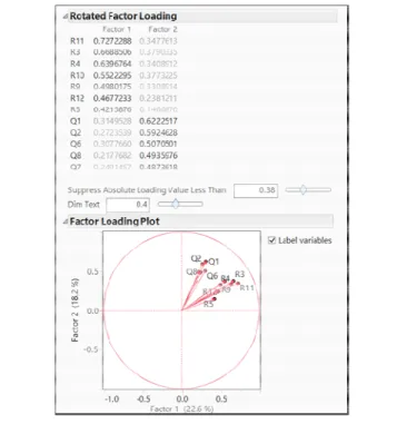
One may suspect that Q13 and Q14 do not belong to the original two factors, and thus they form a third factor. However, this is not the case. Figure 6 shows that Q13 and Q14 were not loaded onto any factor. Even if the loading value was increased to .38 before, Q9 became a one-item factor (Figure 10). In short, the two undetected and misfit items damaged the factor structure.

Figure 10. Factor loadings and loading plot of 14 items for a three-factor solution

When a two-factor solution was imposed on the data, it is obvious that Q13 and Q14 do not belong to any construct (see Figure 11).

Vol 21, No 1

Visualization

With the presence of two problematic items, EFA

factor solution (see Figure 9); this factor structure.

Eigenvalue and Scree plot of 14 items.

One may suspect that Q13 and Q14 do not belong to the original two factors, and thus they form a third factor. However, this is not the case. Figure 6 shows oaded onto any factor. Even if the loading value was increased to .38 as item factor (Figure 10). In short, the two undetected and misfit items damaged the

Factor loadings and loading plot of 14 items

factor solution was imposed on the data, it is obvious that Q13 and Q14 do not belong to

Figure 11. Factor loadings and loading plot of 14 items for a two-factor solution.

Confirmatory Factor Analysis

Interestingly, with such a large sample size the fitness indices of confirmatory factor analysis (CFA) also fail to alert the analyst about the existe

problematic items. CFA was run with SAS 9.4 (SAS Institute, 2014) on the original 12 items of the CFCS and results supported the proposed two

structure (see Table 1). The Adjusted Goodness of Fit Index (AGFI) results (.94) support the propose factor structure, since AGFI values are considered satisfactory when greater than .90 (Hooper, Coughlan, & Mullen, 2008). Steiger (2007) suggest

Mean Square Error of Approximation (RMSEA) is acceptable when less than .07, and Hu and Bentler (1999) stated that the Standardized Root Mean Square Residual (SMSR) is sufficient when less than .08. Both the RMSEA (.06) and SMSR (.03) resul

these suggested thresholds. Together, these fit indices suggest that the two-factor solution is a better fit than the original 12 item CFCS.

Table 1.CFA results for original 12 items AGFI

Parsimonious GFI RMSEA Estimate SRMR

Akaike Information Criterion

In order to assess the impact of the two problematic items (Q13 and Q14) on the factor structure of the CFCS, a separate CFA was run on the scale, which included questions 13 and 14 (see Table 2). Page 6

Factor loadings and loading plot of 14 items

Confirmatory Factor Analysis

Interestingly, with such a large sample size the fitness indices of confirmatory factor analysis (CFA)

fail to alert the analyst about the existence of problematic items. CFA was run with SAS 9.4 (SAS Institute, 2014) on the original 12 items of the CFCS and results supported the proposed two-factor structure (see Table 1). The Adjusted Goodness of Fit Index (AGFI) results (.94) support the proposed two factor structure, since AGFI values are considered satisfactory when greater than .90 (Hooper, Coughlan, & Mullen, 2008). Steiger (2007) suggested that the Root Mean Square Error of Approximation (RMSEA) is acceptable when less than .07, and Hu and Bentler that the Standardized Root Mean Square Residual (SMSR) is sufficient when less than .08. Both the RMSEA (.06) and SMSR (.03) results were within these suggested thresholds. Together, these fit indices factor solution is a better fit than CFA results for original 12 items

0.9448 0.7448 0.0632 0.0330 3126.5051

In order to assess the impact of the two problematic items (Q13 and Q14) on the factor structure of the CFCS, a separate CFA was run on the scale, which included questions 13 and 14 (see Table 2).

(8)

All results from the AGFI (.96), RMSEA (.05), and

SMSR (.03) indices meet the cut-off criteria. Therefore, the proposed two-factor structure for the 14

would be considered acceptable. The Akaike Information Criterion (AIC) result for the original 12 item scale (3126.51) did not greatly differ from the A of the 14-item scale (3152.86). Together, these results show that CFA failed to detect the problematic items (Q13 and Q14).

Table 2. CFA results on 14-item scale including Q13 and Q14

AGFI

Parsimonious GFI RMSEA Estimate SRMR

Akaike Information Criterion

As mentioned previously, MIRT is a synthesis of factor analysis and IRT. Nonetheless, when problematic items exist in the data set Cronbach’s Alpha, EFA, or CFA may fail to detect them initially. This problem would carry over to MIRT even though the polychoric correlation matrix was utilized in SAS. The polychoric correlation matrix is especially useful for analyzing items on self-report surveys, such as personality inventories that often use rating scales with a small number of response categories (e.g. 5 Likert scale). Pearson’s r works best with a high degree of variability. When the distribution of the item responses is narrow due to limited options, the between-item relationships tend to be attenuated in the Pearson’s correlation matrix. Factor analysis based on the polychoric matrix is supposed to reduce these types of statistical artifacts (Lee, Poom & Bentler, 1995; Tello, Moscoso, García, & Chaves, 2006). However, MIRT still suggests a 3-factor solution as EFA did before (see Figure 12 and Table 3).

Figure 12. Scree plot from PROC IRT for CSCF items. Vol 21, No 1

Visualization

All results from the AGFI (.96), RMSEA (.05), and

off criteria. Therefore, factor structure for the 14-item scale would be considered acceptable. The Akaike Information Criterion (AIC) result for the original 12 -item scale (3126.51) did not greatly differ from the AIC

item scale (3152.86). Together, these results show that CFA failed to detect the problematic items

item scale including Q13 0.9557 0.7878 0.0525 0.0286 3152.8633

As mentioned previously, MIRT is a synthesis of factor analysis and IRT. Nonetheless, when problematic items exist in the data set Cronbach’s Alpha, EFA, or CFA may fail to detect them initially. This problem would carry over to MIRT even though oric correlation matrix was utilized in SAS. The polychoric correlation matrix is especially useful report surveys, such as personality inventories that often use rating scales with a small number of response categories (e.g. 5-point works best with a high degree of variability. When the distribution of the item responses is narrow due to limited options, the item relationships tend to be attenuated in the alysis based on the polychoric matrix is supposed to reduce these types of statistical artifacts (Lee, Poom & Bentler, 1995; Tello, Moscoso, García, & Chaves, 2006). However, factor solution as EFA did

Scree plot from PROC IRT for CSCF items.

Table 3 is the output of the interpret parameter estimates of all 14 items yielded by PROC IRT. All p values are less than .0001, and the patterns of the slopes and standard errors of all items

viewing the table alone, even experienced researchers may not be able to tell that Q13 and Q14 contain messy data.

Table 3.Interpret parameter estimates of all 14 items yielded by PROC IRT

Item Parameter Estimate Q1 Intercept1 5.16127 Intercept2 2.88533 Intercept3 2.02889 Intercept4 -1.88742 Q2 Intercept1 2.63126 Intercept2 1.09539 Intercept3 0.20938 Intercept4 -2.20241 R3 Intercept1 3.95101 Intercept2 0.91459 Intercept3 0.16281 Intercept4 -2.58373 R4 Intercept1 3.62955 Intercept2 0.86535 Intercept3 0.10111 Intercept4 -2.36039 R5 Intercept1 1.43904 Intercept2 -0.68285 Intercept3 -1.32029 Intercept4 -2.89727 Q6 Intercept1 3.41807 Intercept2 1.55048 Intercept3 0.86638 Intercept4 -1.3699 Q7 Intercept1 4.2757 Intercept2 2.42502 Intercept3 1.69437 Intercept4 -0.96843 Q8 Intercept1 3.66918 Intercept2 1.80879 Intercept3 0.3596 Intercept4 -1.75766 R9 Intercept1 3.49884 Intercept2 1.13264 Intercept3 0.45408 Intercept4 -1.7882 R10 Intercept1 3.84987 Intercept2 1.28205 Intercept3 0.53106 Intercept4 -2.05369 R11 Intercept1 4.67062 Intercept2 1.29876 Intercept3 0.4193 Intercept4 -2.79894 R12 Intercept1 2.85794 Intercept2 0.63506 Intercept3 -0.58329 Intercept4 -2.63574 Q13 Intercept1 1.3547 Page 7

Table 3 is the output of the interpret parameter estimates of all 14 items yielded by PROC IRT. All p -values are less than .0001, and the patterns of the slopes and standard errors of all items look alike. By viewing the table alone, even experienced researchers may not be able to tell that Q13 and Q14 contain

Interpret parameter estimates of all 14 Estimate Std. Error p 0.10362 <.0001 0.06246 <.0001 0.04878 <.0001 1.88742 0.04569 <.0001 0.0393 <.0001 0.02646 <.0001 0.02314 <.0001 2.20241 0.0345 <.0001 0.05552 <.0001 0.02793 <.0001 0.02581 <.0001 2.58373 0.04005 <.0001 0.0549 <.0001 0.02733 <.0001 0.0249 <.0001 2.36039 0.03969 <.0001 0.02273 <.0001 0.68285 0.01947 <.0001 1.32029 0.02192 <.0001 2.89727 0.035 <.0001 0.04184 <.0001 0.02507 <.0001 0.02194 <.0001 0.02412 <.0001 0.07396 <.0001 0.04563 <.0001 0.03612 <.0001 0.96843 0.02771 <.0001 0.04637 <.0001 0.02653 <.0001 0.02015 <.0001 1.75766 0.02598 <.0001 0.05493 <.0001 0.02821 <.0001 0.0242 <.0001 0.03381 <.0001 0.05021 <.0001 0.02656 <.0001 0.02349 <.0001 2.05369 0.03148 <.0001 0.06848 <.0001 0.03184 <.0001 0.02788 <.0001 2.79894 0.04531 <.0001 0.03429 <.0001 0.01991 <.0001 0.58329 0.01981 <.0001 2.63574 0.03177 <.0001 0.02035 <.0001

(9)

Intercept2 0.40542 0.01677 Intercept3 -0.41711 0.01679 Intercept4 -1.36453 0.02041 Q14 Intercept1 2.19625 0.02737 Intercept2 0.85683 0.01796 Intercept3 -0.82922 0.01786 Intercept4 -2.19915 0.02741

Detection by Data Visualization

When a sample size is small, one may be able to detect problematic items by viewing a scatterplot of total scores (the average of all items except the item under investigation), along with the scores for each item. When a sample size is large, however, data points jam together. This makes pattern recognition difficult and sometimes even impossible (see Figure 13). This issue is known as over-plotting.

Figure 13. Over-plotting: Patterns are hidden in the scatterplot when data points are displayed.

Method

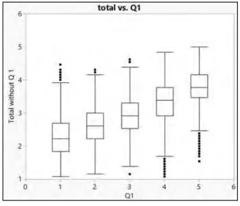
The remedy to this problem is ‘median smoothing’ – that is, changing the display of individual data points to summarized box plots (Tukey, 1977; Yu & Behrens, 1995; Yu, 2014). Figure 14 displays usage of this technique, indicating the relationship between Q1 and the total without Q1. The boxplots in this figure summarize totals at different levels of Q1 scores. This figure clearly indicates that the medians and boxes for Q1 indicate an upward trend; this trend is consistent with the total response pattern in Q1-Q12. Figure 15 indicates another example of this response pattern.

Vol 21, No 1 Visualization <.0001 <.0001 <.0001 <.0001 <.0001 <.0001 <.0001

When a sample size is small, one may be able to detect problematic items by viewing a scatterplot of total scores (the average of all items except the item the scores for each item. When a sample size is large, however, data points jam together. This makes pattern recognition difficult and sometimes even impossible (see Figure 13). This

are hidden in the

The remedy to this problem is ‘median smoothing’ that is, changing the display of individual data points to summarized box plots (Tukey, 1977; Yu & Behrens, displays usage of this technique, indicating the relationship between Q1 and the total without Q1. The boxplots in this figure summarize totals at different levels of Q1 scores. This figure clearly indicates that the medians and boxes for pward trend; this trend is consistent Q12. Figure 15 indicates another example of this response pattern.

Figure 14. Median smoothing of total without Q1 by Q1

Figure 15. Median smoothing of total without Q2 by Q2

Figures 16 and 17 indicate that the preceding trend is absent in both Q13 and Q14. In short, this graphical inspection enables researchers to spot problematic items that Cronbach’s Alpha and factor analysis failed to detect.

Page 8

Median smoothing of total without Q1 by

. Median smoothing of total without Q2 by

Figures 16 and 17 indicate that the preceding trend is absent in both Q13 and Q14. In short, this graphical inspection enables researchers to spot problematic items that Cronbach’s Alpha and factor analysis failed

(10)

Conclusion

In this paper, we illustrated how data visualization can be utilized to identify errors prior to modeling. We used MIRT as an example, due to the fact that IRT is inherently a visual procedure, meaning that interpretation of it necessitates various graphs item-person map, item characteristic curve, item information function curve, test information function curve, and many others). However, very often data visualization of IRT is performed by psychometricians after modeling instead of being used as a d

prior to parameter estimation. It is important to mention that the principle of data visualization is in

Vol 21, No 1

Visualization

Median smoothing of total without Q13 by

In this paper, we illustrated how data visualization can be utilized to identify errors prior to modeling. We used MIRT as an example, due to the fact that IRT is inherently a visual procedure, meaning that interpretation of it necessitates various graphs (i.e. person map, item characteristic curve, item information function curve, test information function curve, and many others). However, very often data visualization of IRT is performed by psychometricians after modeling instead of being used as a diagnosis tool prior to parameter estimation. It is important to mention that the principle of data visualization is in

alignment with the philosophy of exploratory data analysis, which emphasizes examining the data structure, checking assumptions, spotting

fixing errors before committing the data to confirmatory data analysis (Behrens & Yu, 2003; Turkey, 1977; Yu, 2010). The preceding example illustrates that sometimes even random noise could be mis-identified as structure. Despite the versati

MIRT, users who work with large data sets are advised against jumping into usage of MIRT without having first conducted a preliminary item removal. While reliability analysis may fail to identify problematic items, data visualization (such as media

effective for unveiling hidden problems.

References

Adams, R. J., Wilson, M., & Wang, W. C. (1997). The multidimensional random coefficient m

model. Applied Psychological Measurement

Baker, F. B. (1992). Item response theory

Marcel Dekker.

Behrens, J. T., & Yu, C. H. (2003). Exploratory data analysis. In J. A. Schinka & W. F. Velicer, (Eds.),

psychology Volume 2: Research methods in psychology

64). New Jersey: John Wiley & Sons, Inc.

Boyd, J. (2015). Contour (isolines) plots. Retrieved from

http://www-personal.umich.edu/~jpboyd/eng403_chap4_contourp lts.pdf

Carr, D. B., & Nicholson, W. L. (1988). Explor4: A program for exploring four–dimensional data using Stereo Glyphs, dimensional constraints, rotation, and masking. In W. S. Cleveland & M. E. McGill (Eds

graphics for statistics (pp.309–329). Belmont, CA: Wadsworth.

Cleveland, W. S. & McGill, R. (1984). The many faces of a scatterplot. Journal of the American Statistical Association

79, 807–822.

Cleveland, W. S. (1993). Visualizing data

AT&T Bell Lab.

Comrey, A. L., & Lee, H. B. (1992).

analysis. Hillsdale, NJ: Erlbaum. Embretson, S., & Reise, S. (2000).

psychologists. New York, NY: Psychology Press.

Few, S. (2009). Now you see it: Simple visualization techniques for quantitative analysis. Oakland, CA: Analytics Press.

Page 9

alignment with the philosophy of exploratory data analysis, which emphasizes examining the data structure, checking assumptions, spotting outliers, and fixing errors before committing the data to confirmatory data analysis (Behrens & Yu, 2003; Turkey, 1977; Yu, 2010). The preceding example illustrates that sometimes even random noise could be identified as structure. Despite the versatility of MIRT, users who work with large data sets are advised against jumping into usage of MIRT without having first conducted a preliminary item removal. While reliability analysis may fail to identify problematic items, data visualization (such as median rendering) is effective for unveiling hidden problems.

References

Adams, R. J., Wilson, M., & Wang, W. C. (1997). The multidimensional random coefficient multinomial logit

Applied Psychological Measurement, 21(1), 1-23.

Item response theory. New York, NY:

Behrens, J. T., & Yu, C. H. (2003). Exploratory data analysis. In J. A. Schinka & W. F. Velicer, (Eds.), Handbook of psychology Volume 2: Research methods in psychology (pp. 33-64). New Jersey: John Wiley & Sons, Inc.

Boyd, J. (2015). Contour (isolines) plots. Retrieved from

personal.umich.edu/~jpboyd/eng403_chap4_contourp

cholson, W. L. (1988). Explor4: A program dimensional data using Stereo–Ray Glyphs, dimensional constraints, rotation, and masking. In W. S. Cleveland & M. E. McGill (Eds.), Dynamic

329). Belmont, CA:

Cleveland, W. S. & McGill, R. (1984). The many faces of a

Journal of the American Statistical Association,

Visualizing data. Murray Hill, NJ:

Comrey, A. L., & Lee, H. B. (1992). A first course in factor

. Hillsdale, NJ: Erlbaum.

Embretson, S., & Reise, S. (2000). Item response theory for

. New York, NY: Psychology Press.

Now you see it: Simple visualization techniques for

(11)

Hartig, J., & Hohler, J. (2009). Multidimensional IRT models

for the assessment of competencies. Studies in Educational Evaluation, 35, 57-63.

Heveya, D. Pertla, M., Thomasa, K., Maherb, L., Craigb, A., & Chuinneagain, N. (2010). Consideration of future consequences scale: Confirmatory factor analysis.

Personality and Individual Differences, 48, 654–657. Hooper, D., Coughlan, J., & Mullen, M. (2008) Structural

equation modeling: Guidelines for determining model fit. Electronic Journal of Business Research Methods, 6(1), 53-60.

Hu, L. T., & Bentler, P. M. (1999). Cutoff criteria for fit indexes in covariance structure analysis: Conventional criteria versus new alternatives. Structural Equation Modeling: A Multidisciplinary Journal, 6(1), 1-55.

Hulin, C. L., Lissak, R. I., & Drasgow, F. (1982). Recovery of two- and three parameter logistic item characteristic curves: A Monte Carlo study. Applied Psychological Measurement, 6, 249-260.

Hutcheson, G., & Sofroniou, N. (1999). The multivariate social scientist: Introductory statistics using generalized linear models. Thousand Oaks, CA: Sage Publications.

Joireman, J., Balliet, D., Sprott, D., Spangenberg, E., & Schultz, J. (2008). Consideration of future

consequences, ego-depletion, and self-control: Support for distinguishing between immediate and CFC-future sub-scales. Personality and Individual Differences, 48, 15-21.

Joireman, J., Shaffer, M., Balliet, D., & Strathman, A. (2012). Promotion orientation explains why future oriented people exercise and eat healthy: Evidence from the two-factor consideration of future consequences 14 scale. Personality and Social Psychology Bulletin, 38, 1272-1287.

Joireman, J., Strathman, A., & Balliet, D. (2006). Considering future consequences: An integrative model. In L. Sanna & E. Chang (Eds.), Judgments over time: The interplay of thoughts, feelings, and behaviors (pp. 82-99). Oxford: Oxford University Press.

Kamata, A. & Bauer, D. (2008). A note on the relation between factor analytic and item response theory models. Structural Equation Modeling, 15, 136–153. Lai, J., Cella, D., Chang, C. H., Bode, R. K., & Heinemann,

A. W. (2003). Item banking to improve, shorten and computerize self-reported fatigue: An illustration of steps to create a core item bank from the FACIT-Fatigue scale. Quality of Life Research, 12, 485–501.

Lee, S.-Y., Poon, W. Y., & Bentler, P. M. (1995). A two-stage estimation of structural equation models with continuous and polytomous variables. British Journal of Mathematical and Statistical Psychology, 48, 339–358. MacCallum, R. C., Widaman, K. F., Preacher, K. J., & Hong

S. (2001). Sample size in factor analysis: The role of model error. Multivariate Behavioral Research, 36, 611-637. Mihalisin, T., Timlim, J., & Schwegler, J. (1991).

Visualization and analysis of multi–variate data: A technique for all fields. In G. M. Nielsen & L.

Rosenblum (Eds.) Proceedings of 1991 IEEE Visualization Conference (p.171–178). Los Alamitos, CA: IEEE. Mundfrom, D., Shaw, D., & Ke, T. L. (2005). Minimum

sample size recommendations for conducting factor analyses. International Journal of Testing, 5, 159-168. Nikolausa, S, Bodea, C., Taala, E., Oostveenb, J., Glasc, C.,

& van de Laara, M. (2013). Items and dimensions for the construction of a multidimensional computerized adaptive test to measure fatigue in patients with rheumatoid arthritis. Journal of Clinical Epidemiology, 66, 1175-1183.

Samejima, F. (1969). Estimation of a latent ability using a response pattern of graded scores. Psychometrika Monographs, 34 (Suppl. 4).

SAS Institute. (2014). SAS 9.4 [Computer software]. Cary, NC: Author.

SAS Institute. (2015). JMP 12 [Computer software]. Cary, NC: Author.

Schilling, M. F., & Watkins, A. E. (1994). A suggestion for sunflower plots. American Statistician, 48, 303–305. Steiger, J. H. (2007). Understanding the limitations of global

fit assessment in structural equation modeling.

Personality and Individual differences, 42, 893-898.

Strathman, A., Gleicher, F., Boninger, D. S., & Edwards, C. S. (1994). The consideration of future consequences: Weighing immediate and distant outcomes of behavior.

Journal of Personality and Social Psychology, 66, 742-752. Tello, H., Moscoso, C., García, I., & Chaves, S. (2006).

Training Satisfaction Rating Scale: Development of a measurement model using polychoric correlations.

European Journal of Psychological Assessment, 22, 268-279. Tufte, E. R. (1990). Envisioning information. Cheshire, CT:

Graphic Press.

Tufte, E. R. (1997). Visual explanations: Images and quantities, evidence and narrative. Cheshire, CT: Graphic Press.

(12)

Tufte, E. R. (2001). The visual display of quantitative information.

Cheshire, CT: Graphic Press.

Tufte, E. R. (2006). Beautiful evidence. Cheshire, CT: Graphic Press.

Tukey, J. W. (1977). Exploratory data analysis. Reading, MA: Addison-Wesley Publishing Company.

Wang, W. C., Yao, G., Tsai, Y. J., Wang, J. D., & Hsieh, C. L. (2006). Validating, improving reliability, and estimating correlation of the four subscales in the WHOQOL-BREF using multidimensional Rasch analysis. Quality of Life Research, 15, 607-620.

Wolfram, Inc. (2013). Mathematica (version 9) [Computer software]. Champaign, IL: Author.

Wright, B. D., & Mok, M. M. C. (2000). Rasch models overview. Journal of Applied Measurement, 1(1), 83-106. Yan, Z., & Mok, M. M. C. (2012). Validating the coping

scale for Chinese athletes using multidimensional Rasch analysis. Psychology of Sport and Exercise, 13(3), 271-279.

Yu, C. H. (2013). A simple guide to the item response theory (IRT) and Rasch modeling. Retrieved from

http://www.creative-wisdom.com/computer/sas/IRT.pdf

Yu, C. H. (2010). Exploratory data analysis in the context of data mining and resampling. International Journal of Psychological Research, 3(1), 9-22. Retrieved from

http://revistas.usb.edu.co/index.php/IJPR/article/vie w/819 .

Yu, C. H. (2014). Dancing with the data: The art and science of data visualization. Saarbrucken, Germany: LAP. Yu, C. H., & Stockford, S. (2003). Evaluating spatial- and

temporal-oriented multi-dimensional visualization techniques for research and instruction. Practical Assessment, Research & Evaluation, 8(17). Retrieved from

http://pareonline.net/getvn.asp?v=8&n=17

Yu, C. H., & Behrens, J. T. (1995). Applications of scientific multivariate visualization to behavioral sciences.

Behavior Research Methods, Instruments, and Computers, 27, 264-271.

Citation:

Yu, Chong Ho, Douglas, Samantha, Lee, Anna, & An, Min. (2016). Data visualization of item-total correlation by median smoothing. Practical Assessment, Research & Evaluation, 21(1). Available online:

http://pareonline.net/getvn.asp?v=21&n=1 Corresponding Author

Chong Ho Yu, Ph.D. Department of Psychology Azusa Pacific University 901 E. Alosta Ave Azusa Pacific University Azusa CA 91702