A Dissertation by
JIANPING HUA
Submitted to the Office of Graduate Studies of Texas A&M University
in partial fulfillment of the requirements for the degree of DOCTOR OF PHILOSOPHY
December 2004
A Dissertation by
JIANPING HUA
Submitted to Texas A&M University in partial fulfillment of the requirements
for the degree of
DOCTOR OF PHILOSOPHY
Approved as to style and content by:
Zixiang Xiong
(Chair of Committee) Andrew K. Chan(Member)
Edward R. Dougherty
(Member) Costas N. Georghiades(Member)
Andreas Klappenecker
(Member) (Head of Department)Chanan Singh December 2004
ABSTRACT
Topics in Genomic Image Processing. (December 2004) Jianping Hua, B.E., Tsinghua University, P.R. China;
M.S., Tsinghua University, P.R. China Chair of Advisory Committee: Dr. Zixiang Xiong
The image processing methodologies that have been actively studied and developed now play a very significant role in the flourishing biotechnology research. This work studies, develops and implements several image processing techniques for M-FISH and cDNA microarray images. In particular, we focus on three important areas: M-FISH image compression, microarray image processing and expression-based classification. Two schemes, embedded M-FISH image coding (EMIC) and Microarray BASICA: Background Adjustment, Segmentation, Image Compression and Analysis, have been introduced for M-FISH image compression and microarray image processing, respec-tively. In the expression-based classification area, we investigate the relationship between optimal number of features and sample size, either analytically or through simulation, for various classifiers.
ACKNOWLEDGMENTS
First of all I would like to thank my advisor, Professor Zixiang Xiong, for his steadfast support, constant encouragement and expert guidance in my research. He has pro-vided me an environment conducive to learning and quality research. I have equally deep appreciation to Professor Edward R. Dougherty, for his optimism, extensive knowledge and deep insights. I would also like to thank Professor Andrew K. Chan, Professor Costas N. Georghiades and Professor Andreas Klappenecker for serving as my committee members. I am much indebted to Dr. Qiang Wu who has been of great help during my internship. I would also like to thank Dr. Yidong Chen for the creative talks we had.
Furthermore, I owe my appreciation to the colleagues in the multimedia lab, genomic signal processing lab, wireless lab and Advanced Digital Imaging Research. It is a pleasure to having worked with all of you. In particular I would like to thank Zhongmin Liu, Samuel Cheng, Jianhong Jiang, Tianli Chu, Yong Sun, Zhixin Liu, Yang Yang, Qian Xu, Min Dai, Vladimir Stankovic, Xiaobo Zhou, Yuefei Xiao, Chao Sima, Ashish Choudhary, Ranadip Pal, Sanju Nair, Ivan Ivanov, Ulisses Braga-Neto, Yoganand Balagurunathan, Jun Zheng, Shengjie Zhao, Jing Li, Yu Zhang, Wenyan He, Beng Lu, Zigang Yang, Yan Wang, Xianyou Li, Yu-ping Wang and Tiehan Chen for their sincere help. In addition, I want to thank my friends back in China: Zhiwei You, Wei Wang, Yiduo Yu, Liang Zhang, Pingping Zhuang, Deng Lu, and many many others for your encouragement and friendship.
I would like to express my profound gratitude to my parents and my loving wife, Shaoyan Zhang for their love and support.
Finally, I would like to thank everyone else whose names I have not yet mentioned. Without your generous help and support, I would never have finished this dissertation.
TABLE OF CONTENTS
CHAPTER Page
I INTRODUCTION. . . . 1
A. M-FISH and cDNA Microarray Imaging Technology . . . . 2
B. Issues of Genomic Image Processing . . . 4
C. Organization of the Dissertation . . . 8
D. Main Contributions . . . 9
II M-FISH IMAGE COMPRESSION . . . . 10
A. Wavelet-based Medical Image Coding Schemes and M-FISH Image Compression . . . 10
B. Embedded M-FISH Image Coding (EMIC) . . . 12
1. Segmentation and Shape Coding . . . 13
2. Integer Wavelet Transform . . . 14
a. 2-D Shape-adaptive Integer Wavelet Transform . 14 b. 3-D Integer Wavelet Transform Structure . . . 15
3. Fractional Bit-plane Coding . . . 16
a. Object-based Coding . . . 18
4. Wavelet Coefficient Context Modeling . . . 18
a. A General Approach of Optimal Context Modeling 19 b. Optimal Context Modeling for EMIC . . . 22
C. Experimental Results . . . 28
1. Lossless Coding Performance for the Foreground Objects 28 a. EMIC Results with Different Wavelet Filters and Decomposition Levels . . . 28
b. Comparison with Other Lossless Coding Techniques 29 2. Lossy-to-lossless Coding Performance for the Back-ground Objects . . . 31
a. EMIC Results with Different Wavelet Filters and Decomposition Levels . . . 31
b. Comparison with JPEG-2000 . . . 34
III MICROARRAY IMAGE PROCESSING . . . . 40
A. Overview of Micorarray Image Processing . . . 40
CHAPTER Page
1. Signal Estimation . . . 42
a. Mann-Whitney-test-based Segmentation . . . 44
b. Speeding Up Mann-Whitey-test-based Segmen-tation Algorithm . . . 46 c. Post Processing . . . 49 d. Background Adjustment . . . 50 2. Image Compression . . . 53 a. Data Analysis . . . 53 b. Image Compression . . . 54
C. Experimental Results and Discussion . . . 61
1. Comparisons of Wavelet Filters and Decomposi-tion Levels . . . 62
2. Comparisons of Lossless Compression . . . 64
3. Comparisons of Lossy Compression . . . 66
a. Comparisons Based on l1 and l2 Distortions . . . 67
b. Comparisons Based on Scatter Plots . . . 69
c. Comparisons Based on Gene Expression Data . . 69
IV OPTIMAL NUMBER OF FEATURES . . . . 74
A. Problem Overview . . . 74
B. Analytical Results of Quadratic Discriminant Analysis . . 78
1. Normal Approximation to the Discriminant Distribution 81 2. Determination of the Optimal Number of Features . . 86
3. Experimental Results . . . 92
C. Simulation on Various Classifiers . . . 100
1. Simulation Structure for Synthetic Data . . . 101
2. Simulation Results on Synthetic Data . . . 104
3. Real Patient Data . . . 112
V CONCLUSION . . . . 117
REFERENCES . . . . 119
APPENDIX A . . . . 131
APPENDIX B . . . . 133
LIST OF TABLES
TABLE Page
I Correlation coefficients between the current coefficient and its neighbors. The (6,2) wavelet filters with three-level decomposi-tion are used. The correladecomposi-tions are averaged over eight randomly selected training image sets. The results underDAPI column are obtained when current coefficient is in DAPI channel, andOthers
column when it is in other channels. . . . . 24 II Lossless compression results for the foreground objects of M-FISH
images using EMIC with different integer wavelet filters and de-composition levels. The shown compression ratios are in bits
/pixel/channel and are averaged over the eight test image sets. . . . 29 III Lossless compression results of the foreground objects. The
bit-rates shown are in bits/pixel/channel and are averaged over 88 M-FISH image sets. The (6,2) wavelet filters are used with three
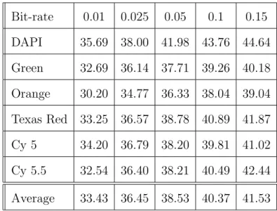
levels of decomposition in EMIC and EWV. . . . . 31 IV PSNR (in dB) of each channel of M-FISH image set “A0101XY”
reconstructed at different bit-rates in bits/pixel/channel. The
(2,4) wavelet filters are used with a five-level decomposition. . . . . . 33 V The comparisons on the number of repetitions between Chen et
al.’s algorithm and our modified method used in BASICA at dif-ferent significance levels. Results are averaged over 504 spots in both channels from different test images. Both algorithms set
m=n= 8 and use the same randomly selected samples from the
predefined background for the Mann-Whitney test. . . . . 49 VI Lossless compression results (in bpp) of BASICA using different
integer wavelet filters with one-level wavelet decomposition. The
TABLE Page VII Lossless compression results (in bpp) of BASICA using the 5/3
wavelet filters with different wavelet decomposition levels. The
results are averaged over the NIH images. . . . . 63 VIII Lossless compression results (in bpp) of different coding schemes. . . 66 IX The equations used in calculating the variance ofaij,i= 1,2, . . . ,7,
j = 1,2, . . . , d and their cross-over terms. The upper-right trian-gle shows the terms among a1j, a2j, . . . , a7j, j = 1,2, . . . , d. The
lower-left triangle shows the terms between a1i, a2i, . . . , a7i and
LIST OF FIGURES
FIGURE Page
1 Two (out of six) channels of a typical M-FISH image set “A0101X”
with size 645× 517 × 6. (a) DAPI channel. (b) Texas Red channel. 3 2 Part of a typical cDNA microarray image in RGB composite
for-mat. . . . . 5
3 Block diagram of the encoder in EMIC for M-FISH image compression. 13 4 Wavelet representation of the foreground objects. (a) The
fore-ground objects of Fig. 1 which include all the chromosomes. (b) The wavelet-domain coefficients after two-level critically sampled
integer wavelet transform of the foreground objects. . . . . 15 5 The 18 8-connected neighbors are categorized into 6 types of
neighbors. These neighboring coefficients and the current coeffi-cient are spanned in three consecutive channels, e.g. DAPI, Spec-trum Green (where the current coefficient locates), and SpecSpec-trum
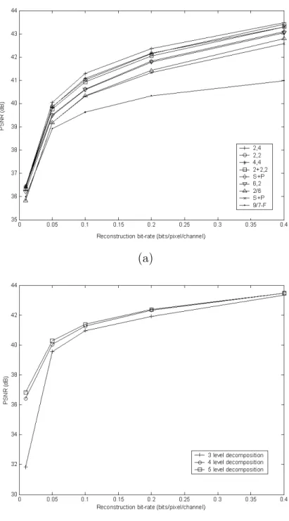
Orange. . . . . 23 6 PSNR performance of EMIC under different wavelet filters and
decomposition levels. The results shown are the average PSNRs of eight sample M-FISH image sets reconstructed at different bit-rates. (a) Comparison between the nine wavelet filters, all with four-level decomposition. (b) Comparison between different levels
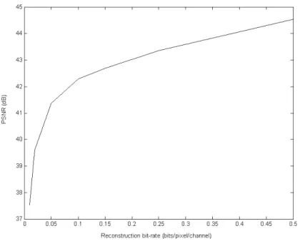
of decomposition using the (2,4) wavelet filters. . . . . 35 7 Average PSNRs from using EMIC for lossy coding of the
back-ground objects at different bit-rate. The results are averaged over
FIGURE Page 8 Two channels of M-FISH image set “A0101XY” reconstructed at
different bit-rates. The images in the left column are from the DAPI channel and the right from the Texas Red channel. (a) The original images. (b) Reconstructed at 0.01 bits/pixel/channel. (c) Reconstructed at 0.025 bits/pixel/channel. (d) Reconstructed at 0.05 bits/pixel/channel. (e) Reconstructed at 0.1 bits/pixel/channel. (f) Reconstructed at 0.15 bits/pixel/channel. The bit-rates
re-ferred are for coding the background only. . . . . 37 9 The major units of BASICA. . . . . 42 10 Segmentation and post-processing of two typical spots. The left
column shows the original microarray spots in RGB composite format. Some intensity adjustments are applied in order to show them clearly. The middle column shows the corresponding seg-mentation results using the Mann-Whitney test with significance level α = 0.001. The right column shows the final segmentation
results after post-processing. . . . . 51 11 (a) Part of a typical cDNA microarray image in RGB composite
format. Some intensity adjustments were applied in order to show
the image clearly. (b) The segmentation results of (a). . . . . 52 12 Rate-distortion curves of log-ratio in terms of (a)l1distortion and
(b)l2 distortion with different wavelet decomposition levels at dif-ferent reconstruction bit-rates. 5/3 wavelet filters were used. The segmentation was performed at three different significance levels
α= 0.001,0.01 and 0.05 and three log-ratios and their correspond-ing distortions were then obtained. The distortions shown are the
averages of the three significance levels over the NIH images. . . . . . 65 13 Rate-distortion curves of log-ratio in terms of l1 distortion (left
column) and l2 distortion (right column) under different recon-struction bit-rates for different compression schemes. (a) Results based on the NIH images. (b) Results based on the SGI images.
FIGURE Page 14 Scatter-plots of log-ratio (left column) and log-product (right
col-umn) estimated from original images and reconstructed images using different schemes. (a) Results based on a NIH image. Black: BASICA at 4.3 bpp; Magenta: BASICA w/o shifts at 4.3 bpp; Green: BASICA w/o PP at 4.7 bpp; Red: JPEG-2000 at 4.0 bpp. (b) Results based on a SGI image. Black: BASICA at 4.1 bpp; Magenta: BASICA w/o shifts at 4.1 bpp; Green: BASICA w/o PP at 4.2 bpp; Red: JPEG-2000 at 4.0 bpp. The significance level
in the Mann-Whitney test is α= 0.05. . . . . 70 15 The disagreement rates vs. the bit-rates. The threshold
parame-ter θ = 1. The segmentation was performed at significance level
α= 0.05. The left column plots depict the detection disagreement rates vs. the bit-rates. The right column plots depict the iden-tification disagreement rates vs. the bit-rates. The disagreement rates shown are the averages of all images. (a) Results based on
the NIH images. (b) Results based on the SGI images. . . . . 73 16 (a) µQ1 d,n vs. d at different λ ’s. n = 40, µ= 1; (b) µQ0d,n vs. d at different µ’s andλ’s. n = 40. . . . . 88 17 (a) µQ0d,n σQ0 d,n vs. d at different µ’s and λ’s. n= 40; (b) µQ1d,n σQ1 d,n vs. d at different µ’s andλ’s. n = 40. . . . . 90 18 Optimal feature size at different sample sizes. All features are
uncorrelated. µ= 1, and λ varies from 1
8 to 8. . . . . 94 19 Optimal feature size at different sample sizes. All features are
uncorrelated. µ= 1
4, and λ varies from 1
8 to 8. . . . . 95 20 Optimal feature size at differentµ’s. All features are uncorrelated.
Sample size is fixed at N = 100, and λ varies from 1
8 to 8. . . . . 96 21 Optimal feature size at differentµ’s. All features are uncorrelated.
Sample size is fixed at N = 40, and λ varies from 1
8 to 8. . . . . 97 22 Optimal feature size at different sample sizes. All features are
equally correlated withρ= 0.2. µ= 1, and λ varies from 1
FIGURE Page 23 Optimal feature size at different µ’s. All features are equally
cor-related with ρ = 0.2. Sample size is fixed at N = 100, and λ
varies from 1
8 to 8. . . . . 99 24 Optimal feature size vs. sample size for LDA classifier. Linear
model is tested. σ2 is set to let Bayes error be 0.05. (a) Uncorre-lated features. (b) Slightly correUncorre-lated features,G= 5, ρ= 0.125.
(c) Highly correlated features,G= 1, ρ= 0.5. . . . . 105 25 Optimal feature size vs. sample size for regular histogram
classi-fier. Uncorrelated features. σ2 is set to let Bayes error be 0.05.. . . . 106 26 Optimal feature size vs. sample size for perceptron and SVM
classifiers. (a) Linear model, uncorrelated features,σ2 is set to let Bayes error be 0.05. (b) Linear model, correlated features,G= 1,
ρ= 0.25. σ2 is set to let Bayes error be 0.05.. . . . 108 27 Optimal feature size vs. sample size for perceptron and SVM
classifiers. Nonlinear model, correlated features,G= 1, ρ= 0.25.
σ2 is set to let Bayes error be 0.05. . . . . 109 28 A case of perceptron classifier: linear model, uncorrelated
fea-tures,σ2 is set to let Bayes error be 0.05. (a) Optimal feature size vs. sample size. (b) Relationship among E[εd(Sn)], E[∆d(Sn)],
and εd for n = 10, 20 and 30. . . . . 111
29 Optimal feature size vs. sample size for 3NN and Gaussian kernel classifiers. Correlated features, G = 1, ρ = 0.25. σ2 is set to let
Bayes error be 0.05. . . . . 113 30 Optimal feature size vs. sample size for 3NN classifiers.
Corre-lated features, G = 1, ρ = 0.25. σ2 is set to let Bayes error be
0.05. . . . . 114 31 Error rate vs. feature size for various classifiers on real patient
CHAPTER I
INTRODUCTION
Since the introduction of the first transgenic plants in 1983, the modern biotechnology has bloomed into a $200 billion industry, extending from pure scientific research into daily merchandises such as food and medicine[1]. In spite of the fiery debate in the ethics aspect, the modern biotechnology exhibits substantial importance to medical research. Nowadays, more than 4000 medical disorders caused by defective genes have been identified, and one out of ten people encounters at least one type of such disorders in his/her lifetime. These facts raise intensive demands in the development of biotechnology in various areas. In treatment, the first case of gene therapy took place in 1990 at NIH. In diagnosis, it is predicted that genetic tests on 25 diseases will be available in most hospitals in 10 years, including commonly seen diseases such as cancer and diabetes. In pharmaceutics, Gleevec, a promising new drug for leukemia, has been put into market. It along with several other drugs reveal the trend of a new generation of medicines designed under the principles of a new science subject named pharmacogenomics. The fast developing technology now exceeds far beyond biology itself, and poses challenging problems in various areas. Due to the multidisciplinary nature of genome-related research, researchers of different backgrounds have been summoned to contribute to this promising field.
Among all these cross-over areas, the methodologies that have been studied and developed by the image processing community – in particular, image processing, com-pression, signal estimation and pattern recognition, are among the most powerful tools for biologists and medical doctors. In modern biotechnology, a huge amount of data
are now obtained in image format, hence raise extraordinary demands on efficient genomic image processing and related data/signal processing. For example, some images for direct inspections by the physicians require highly efficient compression and transmission, and some images for further analysis necessitate accurate informa-tion extracinforma-tion. Also the data obtained through image processing call for powerful signal processing and data mining technology to help biologists understand the true biological meanings behind them. The work proposed here is intended to deal with some of the most important image processing issues associated with two types of genomic image: multiplex fluorescence in situ hybridization (M-FISH) image and cDNA microarray image.
A. M-FISH and cDNA Microarray Imaging Technology
Genome is the smallest element in any living organism that contains all the infor-mation of its cellular structures and activities[2]. Living organism of each biological species has its very own genome, and each cell, the basic working unit of the organism, contains a complete copy of the genome. In each cell, the genome is distributed along the chromosomes, which are the carriers of entwined DNAs. Segments of the DNA with certain nucleotide sequences are called genes, which are expressed or depressed to control the synthesis of protein. The human genome contains about 30,000 genes. M-FISH and microarray imaging technologies are two powerful tools recently devel-oped, which intend to show the properties of genome on the chromosome level and gene level, respectively.
M-FISH imaging is a recently developed technology for molecular cytogenetic analysis [3]. In contrast to the conventional single-staining-based methods, M-FISH specimens are obtained by simultaneous hybridization with a set of chromosome
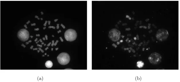
spe-cific DNA probes, each labeled with a different combination of fluorescent dyes. M-FISH images are acquired through a fluorescence microscope with a turret of multiple optical filters for imaging each of the individual fluorescent dyes separately. These are visible in different optical wavelengths referred to as spectral channels. Thus an M-FISH image set is comprised of a number of images, each aligned to the coordinates of a reference image by performing image registration. Fig. 1 shows two (out of six) channels of a typical M-FISH image set.
M-FISH technology enables multi-color karyotyping thanks to the combination of multiple fluorescent dyes used in the chromosome specific DNA probes. Furthermore, it facilitates unambiguous detection of target-specific chromosomal alterations in hu-man and other mammalian cells, which is especially useful for elucidation of subtle or complex chromosomal rearrangements [4]. For these reasons, M-FISH technology has been increasingly used for the diagnosis of genomic abnormalities in the rapidly growing field of cancer cytogenetics.
(a) (b)
Fig. 1. Two (out of six) channels of a typical M-FISH image set “A0101X” with size 645 × 517 × 6. (a) DAPI channel. (b) Texas Red channel.
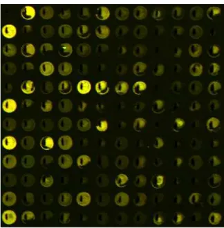
quan-titatively characterize the relative abundance of gene transcripts [5, 6]. Contrary to the conventional methods, microarray technology promises to monitor the tran-script production of thousands of genes or even the whole genome simultaneously. It thus provides a new and powerful tool for genetic research and drug discovery. To produce cDNA microarrays, the mRNA of the control and test samples are first reverse-transcribed into cDNA, and fluorescently labeled with different dyes (typically red and green). Then the fluorescent targets are mixed and allowed to hybridize with gene-specific cDNA clones printed in an array format on a glass microslide. Finally by scanning the microslide with a laser and capturing the photons emitted from different dyes into different channels with a confocal fluorescence microscope, a two-channel 16-bit microarray image is obtained, in which the pixel intensities reflect the level of mRNA expression. Fig. 2 shows a portion of a typical microarray image in RGB composite format, where the red and green channels correspond to the two channels of the microarray image obtained while the blue channel is set to zero. Each round spot in the figure corresponds to the hybridization site of a certain gene. With the techniques from various areas like image processing, classification, clustering, statisti-cal data analysis, etc., cDNA microarray images can shed light on the complex genetic regulation rules long sought by the biologists and clinicians.
B. Issues of Genomic Image Processing
Genomic image processing can be roughly categorized into three major areas: pro-cessing, compression, and analysis. Usually data analysis cannot be performed prior to image processing, while compression sometimes can be performed separately. Basic image processing tasks mainly consist of procedures such as geometric adjustment, noise filtering, segmentation and enhancement. As the very first step of genomic
im-Fig. 2. Part of a typical cDNA microarray image in RGB composite format. age processing, its accuracy is critical to the reliability of subsequent data analysis. Although many genomic images can be analyzed by the biologists directly after pro-cessing, data analysis methods can further help the biologists understand the data from different aspects, and establish a possible link between the data and their biolog-ical meanings. For example, classification can associate the data with certain biologi-cal functions/diseases, hence help the clinicians make diagnosis decisions. Clustering can be used to obtain a holistic view of the data, and to seed a feature selection algorithm for classification. And genetic regulatory networks can help construct the dynamic system involving different genes and suggest the potential medical inter-ventions/treatments. Besides processing and analysis, image compression is another important issue. The images obtained through expensive biological experiments with precious samples need to be archived for later process and double-check, or even being revisited in the future with much advanced technologies. Moreover, current genomic imaging technologies become more and more involved with parallel techniques which
endeavor to provide as much as possible information to the biologists in one shot. For example, both M-FISH and cDNA microarray apply simultaneous hybridizations with multiple fluorescent dyes across a whole set of chromosomes/genes. These fac-tors will significantly increase both the number and the size of the genomic images to be archived. Thus efficient image compression algorithms are highly desired.
It is impractical to perform a thorough research on all the issues. Hence only selected problems in each category are studied in this dissertation:
• M-FISH image compression: Although image compression1 techniques gen-erally fall into two categories: lossy and lossless compression, lossless compres-sion is preferred in most medical applications due to the possibility of informa-tion loss associated with lossy compression[7]. Current method for archiving M-FISH images is to store them channel by channel by losslessly compressing each channel using techniques such as Lempel-Ziv-Welch (LZW) coding [8, 9]. However, M-FISH image has an important characteristic that is distinct from many other types of medical images: it has a foreground which includes infor-mation essential to the diagnosis or analysis, and can be viewed as the region of interest (ROI). On the other hand, the remaining background only provides some reference information. This property opens a door to ROI coding, which encodes the foreground and background independently. In this work we will design a wavelet-based ROI coding scheme for M-FISH image.
• Microarray image processing: Unlike most other medical images, the in-formation of microarray images lies in the intensity of each spot, which is not intended to be analyzed under visual inspection. Thus the signals in microarray 1We use image coding and image compression interchangeably in this dissertation.
images must be estimated with appropriate image processing procedures before any analysis is taken. In this work we will design an efficient microarray signal estimation scheme which can perform a series of basic image processing func-tions, including segmentation and background adjustment, to estimate signals for later analysis.
Besides signal estimation, owing to the large data volume associated with mi-croarray images (each typically takes about 15MB to store), highly efficient compression is necessary. Hence in this work, we will design a good progres-sive compression scheme that provides sufficiently accurate genetic information for data analysis at low bit-rates, while still ensuring good lossless compression performance.
• Expression-based classification: Classification via gene expression level es-timated from the microarray images requires designing a classifier that takes a vector of gene expression levels as input features, and outputs a class label, which predicts the class containing the input feature vector. Given the joint feature-label distribution, increasing the number of features always results in decreased classification error; however, this is not the case when a classifier is designed via a classification rule from sample data. Typically, for fixed sam-ple size, the error of a designed classifier decreases and then increases as the number of features grows. The problem is especially acute when sample size is very small and the potential number of features is very large, which are ex-actly the cases encountered in expression-based classification, where the typical sample size is well under 100, and the available gene expression levels usually up to thousands. Thus it is crucial to obtain a general understanding of the range of feature-set sizes that can provide good performance for a particular
classification rule at certain sample size. In this study we will investigate this relationship for various classifiers.
C. Organization of the Dissertation
The major work accomplished in this dissertation consists of three parts: 1) M-FISH image compression; 2) microarray image processing; 3) determination of the optimal feature size as a function of sample size for expression-based classification.
Chapter II discusses the M-FISH image compression where a new coding scheme, the embedded M-FISH image coding (EMIC), is presented. We first review the shape-adaptive integer wavelet transforms and the object-based bit-plane coding which can generate separate embedded bitstreams that allow continuous lossy-to-lossless com-pression of the foreground and background. Then we propose a method of designing an optimal context model for the bit-plane coding that specifically exploits the sta-tistical characteristics of M-FISH images in the wavelet domain. Experiments have been done to compare our proposed scheme with other popular schemes like LZW coding, JPEG-LS and JPEG-2000.
In Chapter III we target at the microarray image processing for signal estima-tion and image compression. We present Microarray BASICA: an integrated image processing scheme including tools like segmentation, background adjustment and im-age compression for cDNA microarray imim-ages. For the signal estimation part, we first present a fast Mann-Whitney-test-based segmentation algorithm, followed by the post-processing procedure, and finally the background adjustments. For the im-age compression part, we first introduce a new distortion measurement for cDNA microarray image compression and then present a coding scheme by modifying the embedded block coding with optimized truncation (EBCOT) algorithm [10].
Chapter IV investigates the relationship between the optimal number of features and sample size for various classifiers in expression-based classification. Both para-metric and non-parapara-metric classifiers are discussed. First we provide an analytical approach for the quadratic discriminant analysis (QDA) based on the statistic rep-resentation derived by MacFarland and Richards [11]. Then for linear discriminant analysis(LDA) and non-parametric classifiers, we take advantage of the massively parallel computation and perform simulations on the carefully designed distribution models and real patient data.
In Chapter V, we summarize the dissertation on the accomplished works and provide a perspective for the future research in genomic image processing.
D. Main Contributions
• Developed a wavelet-based progressive coding scheme for highly efficient com-pression of M-FISH images. To achieve this, a new context model design method is proposed.
• Designed a microarray image processing scheme, which performs efficient signal estimation and image compression.
• Found an analytic method to determine the optimal number of features at different sample sizes for QDA classifier.
• Studied the optimal number of features as a function of sample size for various classifiers based on both well-designed distribution models and real patient data. A reference web-site is established to provide a resource for the community in assessing the feature-set sizes.
CHAPTER II
M-FISH IMAGE COMPRESSION∗
This chapter presents a new wavelet-based image coder specifically designed for M-FISH image compression. The chapter starts with a brief introduction of the current achievements in wavelet-based image coding, especially in medical image compression. Then our new scheme, embedded M-FISH image coding (EMIC), is discussed in detail.
A. Wavelet-based Medical Image Coding Schemes and M-FISH Image Compression Image compression techniques generally fall into two categories: lossy and lossless compression. Although lossy compression can achieve higher compression ratios, medical diagnosis is often compromised with its usage due to the information loss [7]. Thus lossless compression is preferred in most medical applications. The current method for archiving M-FISH images is to store them channel by channel by losslessly compressing each channel as tiff image using techniques such as Lempel-Ziv-Welch (LZW) coding [8, 9].
However, LZW coding of M-FISH images fails to exploit either the two-dimensional (2-D) pixel correlation within each channel or the dependencies among different chan-nels (each chromosome is located in the same spatial position across different chanchan-nels within an M-FISH image set.) This suggests that standard 2-D JPEG [13] or JPEG-2000 [14] coding would outperform LZW coding and that new 3-D wavelet-based coding techniques [15]-[19] could further improve M-FISH image compression.
Shapiro’s embedded zerotree wavelet (EZW) coder [20] and the later work by
∗°c2004 IEEE. Reprinted, with permission, from “Wavelet-based compression of
m-fish images”, J. Hua, Z. Xiong, Q. Wu, and K. R. Castleman, IEEE Trans. on Biomedical Engineering, to appear.
Said and Pearlman on set partitioning in hierarchical trees (SPIHT) [21, 22] revolu-tionized the field of wavelet image coding. The new JPEG-2000 standard is based on a scheme called embedded block coding with optimal truncation (EBCOT) [10]. Inspired by the success of wavelet image coding, several authors have extended the ex-isting frameworks to 3-D medical volumetric data compression [16, 17, 18, 19, 23, 24], achieving better results than those from the 2-D approaches [25, 26] and the early work of 3-D wavelet-based medical image compression [15]. Among them, 3-D extensions of SPIHT and EBCOT, namely 3-D SPIHT [27] and 3-D embedded subband cod-ing with optimal truncation (3-D ESCOT) [28] achieve the best codcod-ing performance published so far in the literature [17]. An attractive feature of the wavelet-based ap-proach is that, with an integer wavelet transform, one can generate a single embedded bitstream1 that allows progressive lossy-to-lossless compression.
M-FISH images have an important characteristic that is distinct from many other types of medical images: the chromosome regions (the regions of interest to cytoge-neticists for evaluation and diagnosis), which are identical among all channels, are well determined and segmented prior to the storage of each image set. These chro-mosome regions provide diagnostic information and should be losslessly compressed. On the other hand, the remaining background images, which may contain cell nuclei and stain debris, are kept as well in routine cytogenetics lab procedures for specimen reference rather than for diagnostic purposes. Since they usually provide little useful information, lossy compression for them is acceptable. M-FISH images can thus be viewed as consisting of two types of regions of interest (ROI): foreground objects (chromosomes) and background objects (interphase nuclei and stain debris, etc.). 1An embedded bitstream has the property that each additional bit improves the quality of the decoded images and that the whole bitstream can be truncated at any point to provide a set of decoded images with quality commensurate with the bit-rate.
Consequently, regions-of-interest coding [29] should be used to treat the foreground and background objects differently (e.g., lossless coding of the foreground objects and lossy-to-lossless coding of the background objects). In [30], an efficient wavelet-based regions-of-interest coding scheme is already proposed for lossy-to-lossless compression of both the foreground and background objects of single-channel chromosome images. Hence it is natural to apply wavelet-based regions-of-interest coding to M-FISH image compression.
B. Embedded M-FISH Image Coding (EMIC)
In this section we introduce wavelet-based embedded M-FISH image coding (EMIC). EMIC seeks to encode M-FISH images adaptively with respect to the image content. Recall that each M-FISH image set can be classified into two types of ROI: fore-ground objects and backfore-ground objects. Lossless compression is always needed for the foreground objects as they include all the chromosomes, which are essential to cytogeneticists’ evaluation and diagnosis. Lossy compression is acceptable in most cases for the background objects, which contain little diagnostic information. EMIC goes a step further by providing lossy-to-lossless compression for both the foreground and background objects.
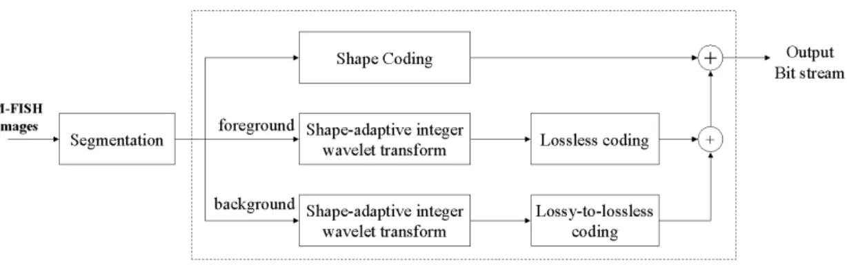
Fig. 3 depicts the block diagram of the encoder in EMIC. A set of M-FISH images is first segmented into the foreground and background objects. This is followed by shape coding of the segmentation mask shared by all image channels. Then we apply critically sampled integer wavelet transforms to both the foreground and background objects, and encode the shapes of the objects as a small header in the bitstream. After the transforms, object-based bit-plane coding is employed to generate one lossless bitstream for the foreground objects and another layered lossy-to-lossless bitstream
for the background objects. In forming the final encoded bitstream, we follow the syntax that the bitstream generated by shape coding goes first, followed by those corresponding to the foreground objects and the background objects, respectively. The encoding procedure is reversed in the decoder. Although we only aim for lossless compression of the foreground and lossy-to-lossless compression of the background, lossy compression of the foreground objects can also be achieved in EMIC by simply decoding at lower bit-rates. The lossy mode is desirable in applications requiring progressive image transmission, such as telemedicine and fast searching and browsing of M-FISH images. The rest of this section describes different components of EMIC in detail.
Fig. 3. Block diagram of the encoder in EMIC for M-FISH image compression.
1. Segmentation and Shape Coding
Before object-based bit-plane coding, segmentation must be performed to delineate the foreground objects from the background objects. EMIC can either use an existing segmentation mask generated interactively under the supervision of cytogeneticists, or obtain it through an adaptive thresholding algorithm (e.g., [31]) applied on the DAPI channel of each M-FISH image set.
Different spectral channels of an M-FISH image set share the same segmentation mask. An 8-connected differential chain code [31] is used to compress the segmenta-tion mask. Shape coding of the segmentasegmenta-tion mask typically costs about 2.5 kbytes per M-FISH image set. Compared to the average lossless compression results on the foreground objects shown later, this overhead due to shape coding is nominal.
2. Integer Wavelet Transform
It was shown in [32] that every finite impulse response wavelet or filter bank can be decomposed into lifting steps. In addition to achieving as much as a two-fold speed-up over filtering-based implementations, the lifting-based approach also makes it very easy to have an integer-to-integer mapping, which is a must for lossless image compression [33]. Different wavelet filters are compared for lossy image compression in [34] and lossless image compression in [35]. In general, the 5/3 filters [33] outperform other wavelet filters for lossless compression, while the Daubechies 9/7 filters [36] are the overall best for lossy compression2. As reported in [33, 35, 37], different wavelet filters excel at different types of images, hence it was not clear which filters are the best for M-FISH images. Thus in Section C we evaluate the 5/3 and 9/7 filters along with seven other commonly used filters [35], i.e., S+P, (2+2,2), (4,2), (2,4), (6,2), (4,4) and 2/6 filters, to experimentally determine the best among this augmented set of filters for M-FISH image compression.
a. 2-D Shape-adaptive Integer Wavelet Transform
After the segmentation of M-FISH images, both the foreground and background ob-jects are arbitrarily shaped, which demands shape-adaptive integer wavelet trans-2These filters are chosen as the default filters for lossless and lossy image compres-sion, respectively, in JPEG-2000 [14].
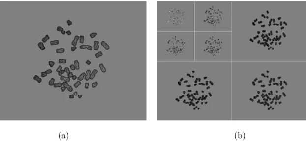
forms. In EMIC, we use odd-symmetric extensions over the ROI boundaries [38]. Fig. 4 shows the foreground objects in Fig. 1 (a) and their two-level critically sam-pled integer wavelet transforms via lifting. It is easy to see that a segmentation mask in the image domain induces a mask for each subband in the transform domain. This wavelet-domain segmentation mask will be used later in the stage of object-based bit-plane coding.
(a) (b)
Fig. 4. Wavelet representation of the foreground objects. (a) The foreground objects of Fig. 1 which include all the chromosomes. (b) The wavelet-domain coefficients after two-level critically sampled integer wavelet transform of the foreground objects.
b. 3-D Integer Wavelet Transform Structure
In 3-D wavelet video coding, we usually use the same wavelet filters in all three dimensions to perform separable wavelet decompositions for both the foreground and background objects. For each object, the 2-D spatial transform and spectral transform (along spectral channels) are done separately by first performing a 2-D dyadic wavelet decomposition on each channel, and then performing a 1-D wavelet decomposition
along the resulting channels3. After the transform, there are eight different types of subbands (e.g., LLL, LLH, LHL, HLL, LHH, HLH, HHL, and HHH bands, where the three alphabets from left to right denote the horizontal, vertical, and spectral dimension, respectively.) Similar to JPEG-2000, after transposing some subbands, we can finally end up with only four types (e.g., LLL, LHL, HHL, and HHH bands.) From our experiments, we find that none of the wavelet filters previously men-tioned can efficiently exploit the correlation across different channels. This can be partially explained by the noticeable difference in the average foreground pixel values across these channels (see Fig. 1). This does not mean those cross-channel co-located pixels are not correlated, they actually are as they correspond to the same set of chromosomes. It merely means that 1-D spectral transform across different M-FISH channels is not an efficient way of exploiting this correlation. Hence in EMIC, we allow the option of not performing the 1-D spectral transform after the 2-D spatial transform of each channel. This option eliminates the spectral highpass bands, such as the HHH bands, and relies on efficient context modeling to exploit the correlation among all six channels in adaptive arithmetic coding [39].
3. Fractional Bit-plane Coding
After the shape-adaptive integer wavelet transform, the wavelet coefficients are com-pressed with bit-plane coding. EMIC employs the bit-plane coding scheme used in embedded wavelet video (EWV) coding [40], which was originally designed for low bit-rate video coding. Below we briefly review the fractional bit-plane coding scheme in EWV which is a 3-D extension of 2-D EBCOT [10] in the JPEG-2000 standard. It offers high compression efficiency and other functionalities (e.g., error resilience and 3The pixel mean of ROIs is subtracted off before wavelet decomposition, as is done in coders like SPIHT [21] and 3-D SPIHT [27].
random access) for image coding. Major components of this scheme are discussed below.
Coding primitives: The state of a coefficient is initially set to insignificant and changed to significant when the coefficient’s first non-zero bit-plane value is encoded. Depending on the states of the nearby coefficients, the current coefficient’s binary information bit at each bit plane is coded using one of the following three primitives: a) Zero coding (ZC): When a coefficient is not yet significant in the previous bit planes, this primitive is used to code whether it becomes significant or not in the current bit plane. b) Sign coding (SC): Once a coefficient becomes significant in the current bit plane, SC is called to code its sign. c) Magnitude refinement (MR): This primitive is used to code the bits of a coefficient if it is already significant.
Fractional bit-plane coding: Using the above three coding primitives in bit-plane coding, one can generate an embedded bitstream for each subband. Specifically, the coding procedure consists of the following three consecutive passes in each bit plane: a) Significance propagation pass: This pass processes coefficients that are not yet significant but have a preferred neighborhood. We use the ZC and SC primitives to code these coefficients’ significance information and, if necessary, their sign bits. b) Magnitude refinement pass: Coefficients that became significant in previous bit planes are coded in this pass. The binary bits are coded by the MR primitive. c) Normalization pass: Processed in this pass are coefficients that are not coded in the previous two passes; these coefficients are not yet significant, so the ZC and SC primitives are applied. Each of the above passes processes one fractional bit plane in the natural raster-scan order.
Bitstream construction and scalability: In this stage, bitstreams corresponding to different subbands will be truncated and multiplexed into a final bitstream. First, an operational R-D curve for each subband can be obtained through the fractional
bit-plane coding. Then, given a target bit-rateR0, optimal rate allocation, i.e., minimum distortion, over all subbands is achieved when operation points on all operational R-D curves have equal slope λ. Lossless coding is achieved by encoding all bit planes, i.e., setting λ to zero. The bitstream with multiple layers is obtained by breaking each subband’s bitstream into multiple layers for different rates, and multiplexing them. Since each subband is coded separately, it can achieve scalability in both rate and resolution with great flexibility.
a. Object-based Coding
The extension of fractional bit-plane coding to shaped-adaptive coding is straight-forward and efficient. The wavelet-domain representation of a typical M-FISH image set’s foreground objects is shown at Fig. 4 (b). Because the shape-adaptive integer wavelet transform is critically sampled, the number of wavelet coefficients is the same as that in the original foreground objects. Using the wavelet-domain segmentation mask, we can easily decide whether a coefficient belongs to the object. If any neighbor of that coefficient falls outside the object, we just set that neighboring coefficient’s value to zero and never code it. The object-based EMIC scheme is inherently better than 3-D SPIHT [27], whose rigid cubic zerotree structure is almost surely inefficient in covering an arbitrarily shaped object.
4. Wavelet Coefficient Context Modeling
The generic context model in [28, 40] for arithmetic coding is designed for natural video sequences. However, for any special class of images like M-FISH data, a generic context model cannot fully exploit the peculiarities that are data specific. Thus, designing a particular context model for M-FISH images is essential for better arith-metic coding performance. In this section we focus on optimizing the context model
in EMIC. We first describe a general approach to optimal context modeling for a given data source. We then explain how to apply this approach to the context model design problem in EMIC.
a. A General Approach of Optimal Context Modeling
Consider a data sequence x1, x2, . . . , xN drawn from alphabet set X of a stationary
random process X. For each sample xi, one can form its context model C using its
preceded samples, i.e., xi−1, ..., x1, x0. Assuming X is anm-th order Markov process, which is reasonable for wavelet-domain image coefficients4, its context model C for
xi can be naturally made up of the m symbols xi−1, ..., xi−m. Then for large N, the
minimum code length (in bits per symbol) is the m-th order conditional entropy,
H(X|C), of X given C [41].
Rissanen has shown in [42] that for a given K-parameter context model C, the minimum model adaptation cost is ∆C = 12(K/N) log2N per symbol. Although a context model with higher K decreases H(X|C) [41], it also induces a higher context model adaptation cost ∆C. For a binary Markov process generated from the
raster-scan of bit planes,K is equal to the number of contexts, i.e., 2m. One way to limit the
model cost is to quantize the 2m contexts intok,k ¿2m, withQ(C)∈ {¯c
1,c¯2, . . . ,c¯k}.
Thus the aim of optimal context modeling is to minimize the average codelength
Lc(X) =H(X|Q(C)) + ∆Q(C). (2.1) To find the optimal context model, one must determine the optimal number of con-texts k, the context decision region Ai = {C : Q(C) = ¯ci} for each context ¯ci, and
the corresponding conditional probability p(X|Q(C) = ¯ci), for 1 ≤ i ≤ k. A direct
4Although wavelet coefficients are almost uncorrelated, there still remains high-order dependencies among them.
approach is to begin with a small k (e.g., k= 2); for eachk, find the optimal context model and compute the corresponding Lc(X); increase k until the model adaptation
cost ∆Q(C) becomes dominant, i.e., untilLc(X) stops decreasing or even increases for
several successive k’s.
For a givenk, the key to optimal context modeling is to find the optimal quantizer
Q(C) that minimizes H(X|Q(C)) in Eq. (2.1). Since H(X|Q(C)) ≥ H(X|C) due to the convexity of the entropy function H(·), it has been shown in [43] that the optimization procedure is equivalent to minimizing
H(X|Q(C))−H(X|C) = X
c
p(c)D(p(X|c)kp(X|Q(c)))
= D(p(X|C)kp(X|Q(C))), (2.2) where D(p(X|c)kp(X|Q(c))) is the relative entropy between p(X|c) and p(X|Q(c)) under a given context c, and D(p(X|C)kp(X|Q(C))) is the conditional relative en-tropy (Kulback-Leibler distance [41]) between the conditional distribution of X given
C and the conditional distribution of X given Q(C).
There is no close-form solution to the problem in Eq. (2.2). However, ifD(p(X|C)k p(X|Q(C))) is viewed as the cost function andD(p(X|c)kp(X|Q(c))) as the distance measure, then it is similar to a hard clustering problem [44]: cluster the contexts into k distinct decision regions to minimize the cost function. Thus the K-means algorithm in classification (or the LBG algorithm in vector quantization [45]) which iteratively updates the decision regions and the conditional probability distributions can be used to find a local-optimal solution. It is shown in [43] that for any context
c with the optimal cluster Q(c) = ¯ci, updating its decision region has to follow the
condition
for any Q0(c) 6= Q(c). Here we point out that updating the conditional
proba-bility distribution p(X|Q(C)) is based on another condition that, for the optimal
p(X|Q(C) = ¯ci) of decision region Ai, X c∈Ai p(c)D(p(X|c)kp(X|Q(c)))≤ X c∈Ai p(c)D(p(X|c)kp0(X|Q(c))) (2.4) for any p0(X|Q(c))6=p(X|Q(c)). This condition can be easily proved from Eq. (2.2).
Below we give a detailed description of the general context clustering algorithm. Cluster 2m contexts into k contexts
• Initialization: Choose an initial set of conditional probability distributions
p(X|Q(C) = ¯c1), . . . , p(X|Q(C) = ¯ck). • Repetition:
– Update the decision regions: for each context c, let
Q(c) = arg min ¯
c D(p(X|c)kp(X|Q(c) = ¯c)). (2.5)
– Update the conditional probability distributions: for each decision region
Ai, let p(X|Q(C) = ¯ci) = arg min q(X|¯ci) X c∈Ai p(c)D(p(X|c)kq(X|c¯i)) = X c∈Ai p(c)p(X|c)/X c∈Ai p(c), (2.6) where the second equation follows the results obtained through the La-grange multiplier method under the constraint Pxq(x|¯ci) = 1. Note that
the optimal probability distribution is the centroid of the current region, which confirms the suggestion in [43].
– Evaluation: compute the cost function D(p(X|C)kp(X|Q(C))) under the current context model parameters.
• Stopping criterion: continue until the cost does not change between two succes-sive iterations.
With this approach, the 2m contexts are clustered intok contexts to form the optimal
context model.
b. Optimal Context Modeling for EMIC
The general approach to context modeling described above assumes the input data sequence is m-th order Markov. In practice, m is not known a priori. Only by determining m first can we correctly form the context model for the current wavelet coefficient.
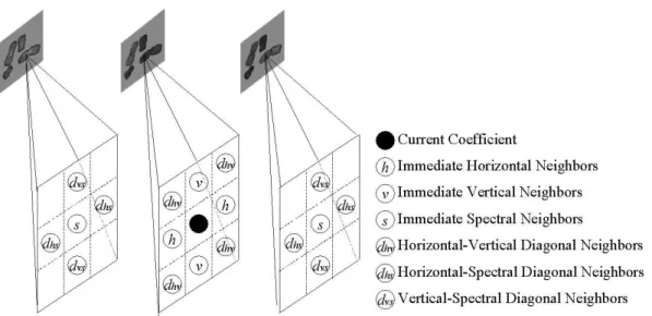
To achieve this, we consider 18 samples in the 3-D neighborhood of the current coefficient (see Fig. 5). We first put these 18 neighbors into 6 categories: immedi-ate horizontal neighbors (h), immediate vertical neighbors (v), immediate spectral neighbors (s), horizontal-vertical diagonal neighbors (dhv), horizontal-spectral
diago-nal neighbors (dhs) and vertical-spectral diagonal neighbors (dvs).
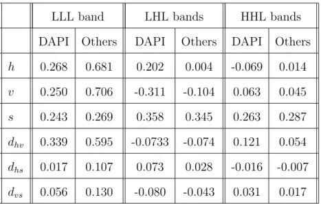
We compute the correlation between the current coefficient and those in each category in different wavelet subbands. The correlation coefficients obtained over eight randomly picked training image sets are shown in Table I. We single out the DAPI channel from other channels because the correlation pattern of DAPI channel is significantly different from other channels. One interesting observation from Table I is that the correlation between the current coefficient and the immediate spectral neighbors is around 0.3 for all subbands and channels. Although these numbers are probably over-estimated due to some isolated pixels with large values, they indicate that there are positive correlations among channels that can be exploited. Another observation is that for all channels except DAPI, the intra-channel correlation is much
Fig. 5. The 18 8-connected neighbors are categorized into 6 types of neighbors. These neighboring coefficients and the current coefficient are spanned in three con-secutive channels, e.g. DAPI, Spectrum Green (where the current coefficient locates), and Spectrum Orange.
higher in the LLL band and drastically lower in other subbands. We also see that the two categories of neighbors dhs and dvs, i.e., horizontal-spectral diagonal neighbors
and vertical-spectral diagonal neighbors, are almost uncorrelated with the current coefficient in all subbands. Thus we drop them and form the context model with the 10 coefficients in the remaining four categories for the ZC primitive. For coding the current coefficient, however, the context model includes all coded bits of the 10 neighboring coefficients. For the SC primitive, like many other coders [14, 46], only the six direct neighbors, i.e., h,v and s neighbors, are involved.
The iterative scheme described in the general approach requires the information of conditional probability distributionp(X|c) for each contextc. However, in practical implementation, this distribution can only be obtained from limited training data. The situation becomes even worse for wavelet-based M-FISH image coding, where the foreground objects are further decomposed into different subbands. The p(X|c)
Table I. Correlation coefficients between the current coefficient and its neighbors. The (6,2) wavelet filters with three-level decomposition are used. The correlations are averaged over eight randomly selected training image sets. The results un-der DAPI column are obtained when current coefficient is in DAPI channel, and Others column when it is in other channels.
LLL band LHL bands HHL bands
DAPI Others DAPI Others DAPI Others
h 0.268 0.681 0.202 0.004 -0.069 0.014 v 0.250 0.706 -0.311 -0.104 0.063 0.045 s 0.243 0.269 0.358 0.345 0.263 0.287 dhv 0.339 0.595 -0.0733 -0.074 0.121 0.054 dhs 0.017 0.107 0.073 0.028 -0.016 -0.007 dvs 0.056 0.130 -0.080 -0.043 0.031 0.017
estimated under limited training symbols can lead to a context model that has good performances only on training images, a problem similar to overfitting in pattern recognition [44]. To avoid this, the total number of contexts should be judiciously chosen to ensure sufficient training symbols in each context. On the other side, since context clustering is an irreversible procedure, special attention must be paid to avoid merging contexts that might belong to different decision regions.
Binary quantization is one way of reducing the context size. A binary-valued state variable σ[i, j, k] that characterizes the significance of coefficient x[i, j, k] at position [i, j, k] is introduced. It is initialized to 0 and toggled to 1 when x[i, j, k]’s first non-zero bit-plane value is encoded. This value is already used in Sec. B.3 of this chapter to decide which coding primitive to use. It quantizes the coded bits of each coefficient in the context model into a binary value, and hence efficiently reduce the
context size. However, with 10 binary symbols in the context, a total of 210 contexts are still too many to obtain reliable p(X|c) in M-FISH context modeling.
There is no reason to treat coefficients in the same category defined in Fig. 5 differently, we thus let h, v, s, and dhv denote the number of coefficients that are
already significant in their own categories. Since the case that most coefficients in one category are simultaneously significant is very rare, we further cap h, v, and s
at one, and dhv at two. With this procedure, the context size is reduced to 24 for
the ZC primitives. And for the LLL and HHL bands, h and v are merged into h+v
and the context size is further reduced to 18. As for the SC primitives, we use the 13 contexts provided in EWV [40]. Although the context size seems relatively small, our experiments show that this is sufficient for coding of the foreground objects.
We point out that the fractional bit-plane coding scheme is actually another type of context clustering. It effectively clusters the contexts into three context state sets, i.e., ZC, SC, and MR primitives, and provides great flexibility by introducing fractional bit planes. It was shown in [47] that the associated performance loss is nominal. Thus our context modeling procedure starts with fractional bit-plane coding and ends with separate optimization of sub-context models for the ZC, SC, and MR primitives. However, whenever there is no confusion, we will still call them context modeling in the sequel.
The general context modeling approach is based on the assumption that the input data sequence is stationary. However, from Table I we see that the data sequence is not stationary (e.g., the DAPI channel and other channels are statistically different). Also the binary sequence generated under the fractional bit-plane coding scheme of EMIC is not stationary among different fractional bit planes.
To ensure the stationarity of the data sequence, we only consider the data from one type of subbands at a time, and treat DAPI channel and other channels
in-dependently. This means that we need to design separate optimal context models for sub-sequences of the data from different subbands and channels. Then for each sub-sequence we convert the binary sequence into a non-binary sequence, where each symbol is made up of the bits from all fractional bit planes, i.e., x = {x1, . . . , xB},
where B is the number of fractional bit planes, and xi is the symbol in fractional bit
plane i. Note that since each bit is coded only once in one of the three fractional bit planes that form that bit plane, xi can actually have three possible values: 1, 0 and
VOID, where the VOID corresponds to the case when no bit is coded in the current fractional bit plane. It is reasonable now to assume that each new input sequence is stationary. Then by assuming that the probability distribution ofxi depends only on
its context, the average codelength can be written as
EX[L(X)] = − N X i=1 X X P(x) log2p(xi|C) = − N X i=1 X X B X j=1 P(x) log2p(xji|Cj) = B X j=1 N ·H(Xj|Cj), (2.7)
whereN now denotes the number of symbols coded in each fractional bit plane. Then the cost function in Eq. (2.2) becomes
H(X|Q(C))−H(x|C) = B X j=1 X c pj(c)D(pj(Xj|c)kpj(Xj|Qj(c))) = B X j=1 D(pj(Xj|Cj)kpj(Xj|Qj(Cj))). (2.8) Although this approach can find the optimal context model for each fractional bit plane, it also scales the total number of contexts by the number of fractional bit planes, which will induce high context adaptation cost. One thus must consider
different fractional bit planes jointly in order to achieve a good balance between the conditional entropy H(X|Q(C)) and the context adaptation cost ∆Q(C).
By observing the training sets of M-FISH images we notice that for each contextc, the conditional probability distribution P(X|c) changes smoothly between adjacent fractional bit planes. This implies that different fractional bit planes can use the same optimal context model to reduce context adaptation cost. Thus in optimizing the context model, we let Qi(c) =Qj(c), 1≤i, j ≤B.
The iterative optimization procedure in Sec. B.4.a of this chapter is used to design the context model for the ZC and SC primitives in different subbands. For the MR primitive, since the refinement bits are known to be almost uniform, EMIC does not perform any context model optimization and keeps the one used in EWV [40]. Separate context models are designed for the DAPI channel and other channels in the LLL, LHL, and HHL subbands. Thus six context models are obtained for each ZC or SC primitive.
The memory usage of the 3-D context model in EMIC is larger than EBCOT’s 2-D model but much smaller than EWV’s 3-D model. Compared to EWV’s generic context model, EMIC only uses a total of 10 neighbors and 6 tables for the ZC primitive. Thus the look-up tables for the ZC context assignment have a maximum of 6×210items, which are 128 times smaller than EWV’s 3×218items for three tables, and are about 6 times larger than EBCOT’s 2×29 items for two tables. Compared to EBCOT and EWV, the look-up tables for the SC primitive in EMIC cost more memory. But since the SC primitive’s context tables are much smaller than the ZC primitive’s, the overall memory cost is actually determined by the latter. As for the complexity issue, setting up the look-up tables takes little time and once it is done, these tables are easy to use. Thus our M-FISH specific context model design does not bring more complexity to the coding procedure than the general context models
in EBCOT or EWV.
C. Experimental Results
Experiments have been conducted to test the performance of EMIC on a total of 88 different M-FISH image sets from a publicly available M-FISH image database (http://www.adires.com /05/Project/MFISH DB/MFISH DB.shtml). Each set has six channels, all with size 645 × 517 and eight bit resolution. These M-FISH image sets belong to the ASI group of test images in the database.
1. Lossless Coding Performance for the Foreground Objects a. EMIC Results with Different Wavelet Filters and Decomposition Levels
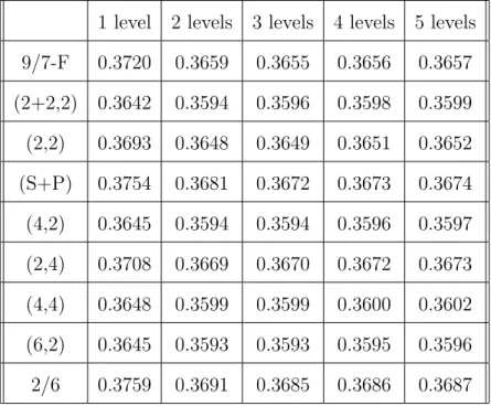
Table II lists the lossless compression results of EMIC with different wavelet filters and decomposition levels. For these tests we randomly selected 8 out of the 88 image sets. We tested all the nine integer wavelet filters mentioned in Sec. B.2.a of this chapter with the level of wavelet decomposition ranging from one to five. From these results we notice that with the same decomposition level, the (2+2,2), (4,2), (4,4), and (6,2) wavelet filters perform closely and they achieve slightly higher compression ratios than the others. For all nine wavelet filters, the compression ratio reaches a peak at the decomposition level of two or three. After that, the compression ratio peaks out and even starts to decrease slightly. Unlike zerotree-based coding schemes, EMIC does not always perform better when the decomposition level increases. This is because the increase in decomposition level results in more small-size subbands. As each subband has its own model-adaptation cost in arithmetic coding, the loss in adaptation cost cancels out the gain from using more decomposition levels at some point. Among the nine wavelet filters and five different decomposition levels, the
(6,2) wavelet filters with a two-level or three-level decomposition performed the best during this test on the eight M-FISH image sets.
Table II. Lossless compression results for the foreground objects of M-FISH images using EMIC with different integer wavelet filters and decomposition levels. The shown compression ratios are in bits /pixel/channel and are averaged over the eight test image sets.
1 level 2 levels 3 levels 4 levels 5 levels 9/7-F 0.3720 0.3659 0.3655 0.3656 0.3657 (2+2,2) 0.3642 0.3594 0.3596 0.3598 0.3599 (2,2) 0.3693 0.3648 0.3649 0.3651 0.3652 (S+P) 0.3754 0.3681 0.3672 0.3673 0.3674 (4,2) 0.3645 0.3594 0.3594 0.3596 0.3597 (2,4) 0.3708 0.3669 0.3670 0.3672 0.3673 (4,4) 0.3648 0.3599 0.3599 0.3600 0.3602 (6,2) 0.3645 0.3593 0.3593 0.3595 0.3596 2/6 0.3759 0.3691 0.3685 0.3686 0.3687
b. Comparison with Other Lossless Coding Techniques
We have compared EMIC against several popular lossless coding schemes: LZW in WinZip 8.0, JPEG-LS, and JPEG-2000. We used the JPEG-LS Reference En-coder V.1.00 implementation by Hewlett-Packard for JPEG-LS coding and Taub-man’s Kakadu V2.2 implementation for JPEG-2000 coding. Because the 2-D based JPEG-LS and JPEG-2000 coders cannot compress the multi-channel M-FISH image set as a whole, the six channels in each set were coded separately when these two
coders were used, and the sums of six compressed file sizes are reported.
Since LZW and JPEG-LS can only handle lossless compression of regularly shaped images, we set the background pixels in test images to zero for these coders. For JPEG-2000, because coding of the foreground and the background is not done separately, no lossless reconstruction of the foreground objects can be guaranteed until the whole image set is recovered. Therefore, the same test images with zero background for LZW and JPEG-LS were used for the JPEG-2000 tests to ensure lossless recovery of the foreground objects. Lossless compression results from differ-ent coders are summarized in Table III. EMIC turns out to perform much better than the other popular coders under study. It achieves an average saving of 78%, 72%, and 17% over LZW, JPEG-2000, and JPEG-LS, respectively. Note that the result of EMIC already includes the overhead of shape coding of the segmentation mask, which, as described in Sec. B.1 of this chapter, is around 2.5 kbytes, or 0.01 bits/pixel/channel for each M-FISH image set. LZW-based WinZip 8.0 gives the poorest result, mainly because it does not take advantage of the 2-D or 3-D structure of the image data. The performance of JPEG-2000 is not very good either because its wavelet transform is not critically sampled, thus more samples need to be coded in the wavelet domain. JPEG-LS performs better than LZW and JPEG-2000 but is still behind EMIC. Furthermore, in contrast to LZW and JPEG-LS, EMIC is capable of providing a scalable lossy-to-lossless bitstream for a given image set. This progres-sive coding property is achieved in EMIC’s encoding process by inserting truncation points to form a layered bitstream. The decoder can simply stop at any truncation point. Bitstream scalability is desirable in applications requiring progressive image transmission, such as in telemedicine and fast browsing of M-FISH images.
Besides the above popular coding schemes, we also provide results based on EMIC with the generic context model from EWV, which we denote as EWV in Table