Technical Efficiency Estimation via Metafrontier Technique with Factors that Affect Supply Chain Operations

(1)

Technical Efficiency Estimation via Metafrontier Technique

with Factors that Affect Supply Chain Operations

Ibrahim Mosaad El-Atroush*

Department of Economics, Tanta University Egypt, Egypt and

Department of Economics, City University London, U.K.

Gabriel Montes-Rojas

Department of Economics, City University London, U.K.

Abstract

This paper presents a metafrontier production function and investigates factors that affect textile and apparel supply chain operations for firms operating under different technologies and ownership structures. Results show variability in efficiency scores. In addition, we find supply chain operations shift the production function and enhance technical efficiency.

Key words: apparel; metafrontier; supply chain variables technical efficiency; textiles JEL classification: C23; C51; D24; L67

1. Introduction

The textiles and apparel (T&A) industry is a sustainable industry which accommodates continual changes in fashions and designs to create new activities and products in highly competitive local and international markets. It has numerous and heterogeneous activities, including converting fibers to fabrics and producing a wide range of products such as technical textiles and apparel. For decades, Egypt has been known as a high quality exporter of raw cottons and cottony products that have been internationally recognized for their unique features. The Egyptian T&A industry is one of the county’s leading sectors, representing greater labor intensity and lower capital intensity relative to other industries. It accounts for 20% of non-oil exports and employs one million workers, representing 30% of the manufacturing workforce and 7% of total employment. The apparel industry is 30% of the T&A employment and women’s apparel is 70% of the total apparel workforce (World Bank, 2006).

*_{Correspondence to: Tanta University, Faculty of Commerce, Said Street, Tanta, Egypt. Email:}

(2)

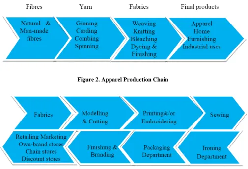
In 2010, exports were USD 3 billion, up more than 6 times since 2004. Private sector firms account for 93% of total exports of apparel, 93% of the total industry’s workforce, 90% of total wages, and 85% of the industry’s capital formation (CAPMAS, 2010). However, Egyptian T&A exports account for less than 1% of global trade in T&A, suggesting that Egypt is not efficiently utilizing its capabilities. The way T&A products are delivered to consumers, in terms of lead time and cost, have changed, with the competitive environment becoming increasingly aggressive (Kilduff, 2000). A typical textiles supply chain has four consecutive phases from raw materials to final products as shown in Figure 1. In contrast, the apparel industry phases from fabrics to retail sales are shown in Figure 2.

Figure 1. Textiles Production Chain

Figure 2. Apparel Production Chain

Although Egypt has comparative advantages in exporting T&A products, its advantages decrease as the process moves down the production chain (Abdelsalam and Fahmy, 2009). The T&A industry has a complete supply chain with many operations that represent separate activities, yet the supply chain does not operate efficiently. Producers face barriers that range from narrow internal efficiency to exhaustive supply chain efficiency. Our primary objective in this article is to study factors that affect Egyptian T&A firms’ supply chain operations and their ability to compete globally. Additionally, producers are struggling to improve their products’ quality to compete in rapidly evolving markets. To do so, producers need to reduce product and service costs, to shorten delivery periods, and to lower inventory costs (Kritchanchai and Wasusri, 2007). A related objective in this article is to measure

(3)

firms’ efficiency scores across geographic regions and to compare them relative to a shared metafrontier then add key factors that affect supply chain operations to assess their impact on efficiency scores. These factors are as follows.

1. Planning for industrial firms (P): an industrial firm’s ability to set plans and strategies aimed at managing its resources that goes towards satisfying customers’ demand for products or services via monitoring supply chain operations efficiently through industrial planning and marketing planning. In this context, good planning yields high quality products with low costs and short lead times.

2. Raw materials or sourcing process (SP): a firm’s ability to follow best purchasing strategies aimed at obtaining cheap and high quality raw materials regardless their source (local or international). This includes ordering and receiving shipments, verifying them, and transferring them to manufacturing units. Thus, efficient sourcing enables the firm to choose among varied sorts of supplies with inexpensive and high quality inputs and avoids bottlenecks in the production process.

3. Hauling or delivery system (DS): the flow of raw materials and final products through a firm, whether it uses its own transport means or hires a service, including developing a network of warehouses and picking carriers to get products to customers. Having an efficient delivery system satisfies customers’ orders within target lead times and enhances the firm’s ability to replenish low inventory in a timely fashion.

4. Inventory and returns system (RS): this factor deals with a firm’s inventory and returns flow. This includes the ability of the firm to control its inventory and minimize customers’ returns and implementing strategies address surpluses via promotions, fairs, and so on. Efficiency in this factor reflects efficient management and structure of the firm.

Visible supply chain operations (SCV) are estimated via a single framework following the Good et al. (1993) methodology in which the impact of SCV shifts the production technology and affects the mean output, where any increase in the mean output enhances efficiency. Thus, the main goals of the paper are to compute comparable technical efficiency ( TE ) for firms operating under different technologies and to examine the roles of factors that affect supply chain operations.

2. Metafrontier Model

For a single output, the technology frontier is defined as a stochastic frontier (SF) production function for R_{different regions within the industry. For} the jth

region, there are data on Nj firms, and its regional SF model is: ( ) ( )

( ) ( ( ), ( )) it j it j

V U

it j it j j

Y = f x β e − , i=1, ,_K N_j, t=1, ,_K T, j=1, ,_K R, (1) where Yit(j) is the output of the ith firm in the tth time period in the jth region,

(4)

) (j it

x is a vector of values of functions of inputs used by the ith firm in the tth time period in the jth region, β(j) is the parameter vector associated with the x

variables for the SF for the jth region, vit(j) is a random error component which is

assumed to be identically and independently distributed as (0, 2 )

) (J V

N σ , and uit(j) is

the inefficiency component which is assumed to be distributed as (0, 2 )

) (j u N+ σ _{. More} precisely, we assume: ) ( ) ( ) ( ) ( ) ( ) , ( () () ) ( j it j it j it j it j it U X V U V j j it j it f x e e Y ₌ _β − _≡ β + − . (2)

The exponent of the production function is linear in the parameter vector β(j) for the

vector of inputs xit for the ith firm in the tth period. Following Battese and Coelli

(1992), the metafrontier production function model for the industry is: * ) , ( * * _β Xitβ it it f x e Y ≡ ≡ , 1 1, , R j j i N N = = _K =

_∑

, t=1, ,_K T, (3)

where β*_{is the vector of parameters for the metafrontier function with:} ) ( * j it it x x β ≥ β . (4)

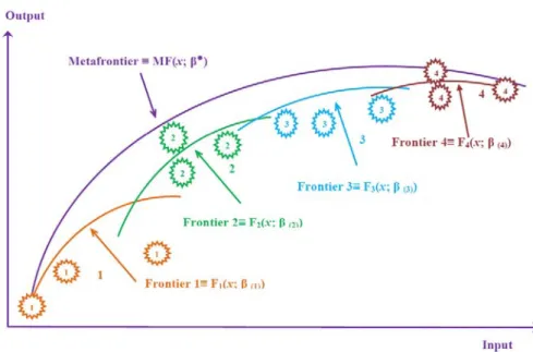
The metafrontier production function values (as a deterministic parametric function) are no smaller than the deterministic components of production functions of different regions and time periods. The metafrontier is assumed to be a smooth function and not a segmented envelope as in Figure 3. For instance, the private firms are illustrated with four SF models representing four regions (Alex, Canal, Delta and G. Cairo firms) as in Figure 3 where observed values are indicated by numbers that relate to the particular regional frontiers and their unobservable stochastic frontier outputs are shown by the numbers above them. The values of the curves corresponding to the circled numbers can be considered as means of the potential stochastic frontier outputs for the given levels of the inputs. Metafrontier function values are no less than the deterministic functions associated with SF models for different groups involved. Some SF outputs may exceed metafrontier values, as can be seen for one of the group 4 points in Figure 3. The same methodology is implemented for other three regions.

Equations (3) and (4) follow Hayami and Ruttan’s (1970) concept of the metaproduction function: “The metaproduction function can be regarded as the envelope of commonly conceived neoclassical production functions” (p. 82). This framework is also consistent with the Battese et al. (2004) model of a metafrontier function where a production function of specified functional form does not fall below the deterministic functions for the SF models of the groups involved. This model assumes that data generation models are only defined for the frontier models for the firms in the different groups. We can obtain maximum likelihood estimates (MLEs) of the parameters of the metafrontier model in (2) and (4) and of the SF for each group such that the estimated function envelops the deterministic components of the estimated SFs. This deterministic metafrontier is solved via linear

(5)

programming (LP).

Figure 3. Metafrontier and Regional SF Functions

Output for the thi firm in the tth time period, defined by the SF for the jth group in (2), is alternatively expressed in terms of the metafrontier of (3) by:

) ( * * ) ( ) ( it itj it j it j it x V x x U it e e e e Y − + × × = β β β . (5)

The first factor in (5) is the TE relative to SF forthe jth region:

) ( ) ( ) ( j it j it j it U V x it it e e Y TE − + = = _β . (6)

The second factor in (5) is the technology gap ratio (TGR) for the observation for the sample firm involved:

* ) ( β β it j it x x it e e TGR = . (7)

The TGR measures the ratio of the output for the frontier production function for the jth group relative to the potential output (the metafrontier function) obtained via observed inputs. It has values between 0 and 1 because of (4). The TE

for the thi firm relative to the metafrontier, denoted * it

(6)

observed output relative to the metafrontier output adjusted for the corresponding random error, i.e., the last factor in (5):

) ( * * j it it V x it it e Y TE = _β₊ . (8)

Equations (5)–(8) imply an alternative expression for the (_TE*_{) relative to the}

metafrontier:

it it

it TE TGR

TE*= × _. ₍₉₎

Thus the TE_{relative to the metafrontier function (}_TE*_{) is the product of}_TE

relative to the regional SF and TGR. Since both TE and TGR are between 0 and 1,

*

TE is also between 0 and 1 but is less than the group TE.

The private firms are situated in four regions: Alex zone firms (Beheira and Alexandria governorates), Canal zone firms (Port Said, Ismailia, Suez, and Sharqia governorates), Delta zone (Dakahlia, Gharbia, Qalyubia, and Monufia governorates), and greater Cairo zone (Cairo and Giza governorates). The public firms are located in three regions: Cairo and Upper Egypt zone (Cairo, Giza, Qalyubia, Minia, Asyut, Sohag, and Qena governorates), Delta zone (Gharbia, Dakahlia, Damietta, and Sharqia provinces), and Alex zone (Alexandria, Behera, and Port Said governorates). Carrying out SF analysis at the regional level is desirable since industry firms in different regions probably operate under different technologies and different ownership structures. Additionally, metafrontier production function estimation for the industry permits us to compare firms’ TE in different regions relative to the metafrontier and to examine technology gaps in particular regions relative to the industry. Empirical results are obtained through the SF production model with time-varying inefficiency effects, proposed by Battese and Coelli (1992). The first Cobb-Douglas SF model, representing the production technology for T&A firms for a specific region, can be expressed as:

it t j l it j m it j k it it K M L Y =β +

_∑

β +

_∑

β +

_∑

β +γ +ε = = = 4 1 4 1 4 1 0 it it it =v −u ε (10)

[

]

{

exp ( )

}

it t i U = −η t T− u. (11)

The merit of the Cobb-Douglas form is that the coefficients βk, βm, and βl

are the output elasticities of the inputs, and their sum provides the elasticity of scale. This form is chosen to characterize the T&A industry for several reasons. First, it has been shown to be theoretically sound and attractive due to its computational feasibility and availability of adequate degrees of freedom for statistical testing (Heady and Dillon, 1969). Second, this assumption avoids multicollinearity present in some activities across sectors. Moreover for public sector firms, there were too few observations to estimate the translog form despite there being large and

(7)

extra-large firms. Selecting this technology form for the region-specific and metafrontier model imposes consistency that is useful for efficiency comparisons.

Finally, the main four variables affecting supply chain operations—P, SP, DS, and RS—are added to the previous model to examine their impacts on the production technology function:

4 4 4 0 1 1 1 4 4 4 4 1 2 3 4 1 1 1 1 . it k it m it l it t j j j it it it it it j j j j Y K M L P SP DS RS β β β β γ α α α α ε = = = = = = = = + + + + + + + + +

∑

(12)

3. Model Justification for the Egyptian T&A Industry

The concept of a stochastic metafrontier function is a modified version of the standard metaproduction function approach which has an error term that comprises a symmetric random error and a nonnegative technical inefficiency. The stochastic metafrontier approach was adopted by Gunaratne and Leung (2001) in a study of the efficiency of aquaculture farms in several countries. It is also possible to use non-stochastic approaches to construct metafrontier functions. The Egyptian T&A industry has unique characteristics, including covering a number of regions with distinct social, economic, and infrastructural features. Easy access to production inputs and other infrastructural facilities (helpful in achieving lower costs per unit of output) is not evenly distributed all over the country (e.g., in G. Cairo and Delta zones). Regions differ widely regarding differences in available stocks of physical and human capital. Social and economic infrastructure, e.g., number of ports, access to markets, business management expertise, roads and electricity, also vary across regions of production. These factors are chief determinants of the level of TE of a firm situated in any particular region. Although the core production function for different regions is the same, these environmental factors cause the underlying production function to shift away from the metafrontier. Therefore, it is appropriate to consider production technology itself as dissimilar across regions.

While geographical factors play an important role in creating differences in the technology across groups of firms, such differences may also arise due to differences in ownership structure and in the organizational structure of a firm. For example, a firm in the public sector may perform differently from one in the private sector even though both are located in same region. In our empirical analysis, we examine the extent of systematic differences in the TE levels of firms due to geographical location and ownership type. We investigate how much variation in these factors affects the levels of TE for individual firms. We also examine whether the production technology itself varies across groups due to variation in these factors by comparing respective TGR.

(8)

4. Description of Variables and Data

Data on Egyptian T&A firms were obtained through annual industrial statistics bulletins of Egyptian T&A firms from the Central Agency of Population, Mobilization, and Statistics (CAPMAS) from 2001 to 2008 for the public firms and from 2006 to 2008 for the private firms covering all firms’ sizes, ages, and activities. These data were combined with those acquired through questionnaires and interviews obtained by the Business Sector Information Centre (BSIC, 2010) to construct the main factors that are hypothesized to affect supply chain operations.

Output (Yit) represents the natural logarithm of the total value of manufacturing

output of the ith firm in the tth year in Egyptian pounds at constant 2001 prices. Labor (Lit) is the natural logarithm of total paid wages per year in Egyptian pounds

at constant 2001 prices (x1). Materials (Mit) are the natural logarithm of total costs

of raw materials purchased by the firm during the year in Egyptian pounds at constant 2001 prices (x2). Capital (Kit) is the natural logarithm of all operating

costs as a proxy of capital, including expenditures on electricity, fuel and lubricants, maintenance and repairs of capital goods, buildings and machinery rents, and machinery upgrading, during the year (x3). And εit is a compound error term

including vit (a two-sided “noise” component) and uit (an inefficiency component).

Both vit and uit are distributed independently of each other and of the regressors.

Factors hypothesized to affect supply chain operations were obtained via questionnaires and available historical information for each firm during a 3-year period for private units and an 8-year period for public entities. Interviews were also conducted with firms’ chief executives, production units’ managers, employees, and workers for both sectors. The questionnaire asked 40 questions relating to supply chain variables: 16 questions about planning processes (8 for marketing planning and 8 for industrial planning), 12 questions for sourcing processes, 6 questions for delivery system processes, and 6 questions for stock and returns process. Additional questions asked about workers numbers, educational levels, and general firm information. All questions were given the same weights (2 for “yes” and 1 for “no”) to calculate factor means for Pit, SPit, Dsit, and Rsit.

The TE of a firm operating under one particular production technology is not necessarily comparable with that of a firm operating under a different production technology. Battese et al. (2004) adopt a model that assumes that there exists only one data-generating process for the firms operating under a given technology. The metafrontier function is a principal function that incorporates the deterministic components of the SF production functions for firms that operate under different technologies. Data cover Egyptian T&A sector firms in three regions for public firms and four for private firms, with 838 private firms (379 textiles and 459 apparel) covering all six T&A activities described below.

1. Yarn: includes natural fibers (e.g., cotton, flax, silk, jute, and wool) and synthetic fibers (e.g., acrylic, polyester, nylon, and viscose).

(9)

2. Weaving: includes cotton weaving, flax weaving, natural and synthetic silk and nylon weaving, jeans weaving, finishing knitting fabrics, other types of knitting fabrics, making fabrics tapes, and other types of weaving.

3. Fabrics: includes bleaching, dyeing, printing, and finishing stages for natural and man-made fibers and home furnishing, underwear, and apparel fabrics. 4. Home furnishing: includes making curtains and table linens, quilts, covers,

bed linens, embroidered home furnishing, blankets making, terry towels, and kitchen towels.

5. Underwear and socks stage: includes men and boys’ underwear, women and girls’ lingerie, knitted underwear, brassieres, boys and girls’ socks, women’s socks, men’s socks, and gloves.

6. The apparel stage: includes suits, shirts, pajamas, T-shirts, men and boys’ wear, women and girls’ wear, kids’ wear, sportswear, swimming wear, leather wear, sewing women wear, sewing men wear, jumpers, and knitting products, other types of knitting wear, sewing domestic wear, scarves, ties, and other types of apparel.

Activities 1–4 belong to textiles and activities 5–6 belong to apparel. The apparel sector is labor intensive with highly differentiated products, while the textiles sector is capital intensive with less differentiated products.

The private firm sample covers includes small (1–25 workers), medium (26– 100 workers), large (101–1000 workers), and extra-large firms (over 1000 workers). It also includes firms that produce for local and global markets. The large and extra-large firms are fully integrated, meaning these firms may be engaged in more than one activity, such as weaving, fabrics, and apparel. Small and medium firms are engaged in at least one activity, and most private firms have their own transport means to obtain industry inputs from suppliers and to deliver products to clients.

Additionally, all 25 firms in the public firm sample are large and extra-large firms with sizes varying from 500 to 21969 workers. The public firms are mainly textiles producers. Their activities range from fully integrated activities covering all T&A supply chain processes to firms engaged in only a single textile process. Each firm also has its own transport means and most firms produce for both local and foreign markets. All data for both sectors about industry inputs and outputs were obtained in current prices then deflated to obtain constant 2001 prices. Separate deflators were used for outputs, wages, raw materials, and capital.

5. Empirical Results 5.1 Private Sector Firms

Empirical results for textile and apparel private firms are illustrated as follows.

5.1.1 Textiles Sector Firms

(10)

firm data combined with data acquired via questionnaires and interviews conducted by the BSIC to construct SCV. Tables 1, 2, and 3 illustrate descriptive statistics for private and public T&A firms. Table 1(a) reports MLEs of the production function for textiles firms. The elasticity of labor is 16%, materials is 58%, and capital is 17% and these firms exhibit decreasing returns to scale without SCV, whereas corresponding values are 19%, 61%, and 21% and these firms show constant returns to scale with SCV. Input coefficients are significant.

Table 1. Summary of Textiles Firm Output, Inputs, P, SP, DS, RS, Size, Age, GB, B, and EXR

Variable Mean Min Max St. Dev.

Output 6.1080 4.2080 8.4700 0.8020 Labor 5.0389 3.9837 7.7694 0.6990 Material 5.8528 3.6593 8.1046 0.8390 Capital 4.8536 2.9789 7.8300 0.8841 Planning 1.5282 1.0400 1.900 0.1717 Sourcing 1.5678 1.0800 1.9500 0.1766 Delivery System 1.5190 1.2000 1.8500 0.1415 Returns System 1.5707 1.2500 1.9400 0.1503 Size 1.0026 0 2 0.8428 Age 0.6174 0 1 0.4862 GB 0.3017 0 1 0.4592 B 0.5154 0 1 0.5000 EXR 0.3289 0 1 0.4700

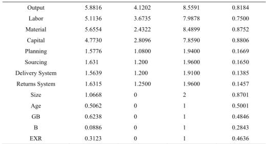
Table 2. Summary of Apparel Firm Output, Inputs, P, SP, DS, RS, Size, Age, GB, B, and EXR

(11)

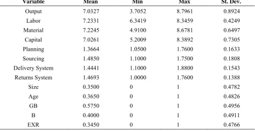
Table 3. Summary of Public Firm Output, Inputs, P, SP, DS, RS, Size, Age, GB, B, and EXR

Table 1(a). MLEs for Production Function Panel Data Time Varying for Textiles Firms

Variable Coefficient Model 1 without (SCV) Model 2 With (SCV) Metafrontier LP (SCV) Constant β0 1.424 (.069)*** 1.396 (.086)*** 1.643 (0.070)*** Labor (Lit) β1 0.156 (0.017)*** 0.192 (.018)*** 0.185 (0.012)*** Material (Mit) β2 0.576 (0.007)*** 0.614 (0.007)*** 0.617 (0.010)*** Capital (Kit) β3 0.173 (0.014)*** 0.213 (0.014)*** 0.201 (0.015)*** Year γt –0.019 (0.011)* –0.018 (.0112)* –0.018 (0.004)*** Planning (Pit) α1 – –0.161 (0.146) –0.156 (0.079)** Sourcing Process (Spit) α2 – 0.148 (0.146) 0.054 (0.083) Delivery System (Dsit) α3 – 0.155 (0.128) 0.174 (0.070)*** Returns System (Rsit) α4 – –0.114 (0.115) –0.056 (0.068)

Estimated Efficiencies Mean Min Max St. Dev.

Efficiency without SCV 0.8384 0.6424 0.9848 0.076 Efficiency with SCV 0.8430 0.6828 0.9884 0.075 Notes: N=1137. *, **, and *** denote significance at 10%, 5%, and 1% levels in a two-tailed test.

Mean TE without SCV is 84% with range 64% to 98%, and the mean with SCV is 84% with range 68% to 99%.

Table 1(b) presents TE, metafrontier _TE*_{, and}_TGR_{ratios for Alex, Delta, G.}

Cairo, and Canal regions. For the Alex region, mean TE without SCV is 70%, _TE*

is 28%, and hence TGR is 40%; with SCV corresponding values are 73%, 33%, and 46%. For the Delta region, mean TE without SCV is 81%, _TE*_{is 63%, and}_TGR

is 78%; with SCV corresponding values are 81%, 66%, and 81%. For G. Cairo region, mean TE without SCV is 88%, _TE*_{is 88%, and}_TGR_{is 100%; with SCV}

(12)

corresponding values are identical. For the Canal region, mean TE is 49%, _TE*_is

5% (which is the lowest across regions), and TGR is 11%; with SCV corresponding values are 86%, 86%, and 100%, meaning that Canal region firms have the highest response to SCV among textiles firms. It is interesting to note that Delta and G. Cairo regional frontiers are tangent to the metafrontier; the maximum value for the technology gap ratio (i.e., 1) was obtained for both regions and for Canal with SCV.

Table 1(b). TGR and TE Regional Frontiers and TE* for Textiles Private Firms Region/statistic Values without SCV Values with SCV

Alex Mean Min Max St. Dev. Mean Min Max St. Dev. Metafrontier TE* 0.2810 0.2622 0.9812 0.0855 0.3322 0.3034 0.9719 0.0824 Regional TE 0.6986 0.4386 0.9837 0.1334 0.7258 0.4933 0.9857 0.1282 TGR 0.4022 0.3978 0.7716 0.1273 0.4577 0.4416 0.8412 0.1013 Delta Metafrontier TE* 0.6680 0.6302 0.9954 0.0438 0.6560 0.6941 0.9988 0.0389 Regional TE 0.8599 0.6615 0.9832 0.0656 0.8764 0.7240 0.9846 0.0609 TGR 0.7786 0.5564 1.000 0.0735 0.8103 0.5816 1.000 0.0543 G. Cairo Metafrontier TE* 0.8564 0.7322 0.9823 0.0357 0.8737 0.7416 0.9818 0.0381 Regional TE 0.8748 0.7343 0.9799 0.0615 0.8740 0.7418 0.9825 0.0611 TGR 0.9790 0.6671 1.000 0.0837 0.9999 0.6973 1.000 0.0766 Canal Metafrontier TE* 0.0544 0.0409 0.9586 0.1923 0.8597 0.6042 0.9648 0.0335 Regional TE 0.4851 0.1289 0.9621 0.2432 0.8598 0.6509 0.9650 0.0713 TGR 0.1122 0.0344 0.6218 0.2513 0.9999 0.6018 1.000 0.0466

After obtaining efficiency scores for each region, the efficiency scores are regressed against firm’s size, age, governmental barriers (GB), bureaucracy (B), and exchange rate (EXR) dummies as regressors. The Hausman test for fixed vs. random effects supports fixed effects model. Regional dummies are also included in the model. Firm size is classified as small, medium, large, and extra large. Firm age is classified as new and old. GB represent governmental barriers which examine their impact on efficiency, B represents bureaucracy to examine its impact on working environment, and EXR examines the impact of exchange rates on efficiency scores.

Table 1(c) shows that these variables are not significant; this is likely because textiles firms are capital intensive. Moreover, the textiles sector is the main provider of the apparel sector inputs, implying what is produced in textiles is sold to the apparel sector as yarn or fabrics. For instance, yarns higher than 36 and 40 gauges are used for producing fine branded apparels and yarns with low ranks or thick yarns such as 20, 16 and 10 gauges are used to produce towels and bed linens, and this may explain the saying that everything produced in textiles sector is sold (i.e., there is no waste). The coefficient of bureaucracy is not significant and this may be due to private sector managers circumventing time-consuming bureaucratic procedures by

(13)

bribery (this explanation is supported by the manager interviews). The coefficient for exchange rates is also not significant; this may be because changes in exchange rates have a minor impact on products pricing. The coefficient for government barriers is not significant; this may be a result of differences in infrastructure and services among regions. Firm size and age are also not significant in this capital intensive sector in which a textile firm with 25 workers is considered large whereas an apparel firm with same number of workers is considered small.

Table 1(c). Regression Results for Textiles Firm TE* against Regions, Size, Age, GB, B, and EXR 2006-2008

Variables Fixed Effects without SCV Fixed Effects with SCV

Alex 0.69D-04 (0.007) 0.57D-04 (0.006) Delta 0.35D-04 (0.007) –0.010 (0.006) G. Cairo –0.0109 (0.007) 0.29D-04 (0.006) Canal 0.007 (0.007) 0.006 (0.006) Size –0.0102 (0.007) –0.009 (0.006) Age 0.71D-04 (0.007) 0.55D-04 (0.006) GB –0.009 (0.007) –0.008 (0.006) B 0.79D-04 (0.007) 0.64D-04 (0.006) EXR –0.008 (0.007) –0.007 (0.006) R2_{% 7.33} _7.31

5.1.2 Apparel Sector Firms

Table 2(a) presents MLEs of apparel private firms. Labor elasticity is 34%, materials are 50%, and capital is 16%, and the firms exhibit constant returns to scale. Labor elasticity supports the fact that the apparel sector is labor intensive. With SCV corresponding values are 38%, 52%, and 20%, indicating increasing returns to scale. Input coefficients are significant at the 1% level, and the sourcing process is significant at the 10% level since raw materials play a major role in input costs where materials represent 60% of the total FOB production cost (Birnbaum, 2005). Mean TE with and without SCV is 99%. This may be because the apparel sector has wide-ranging products, varied production processes, and integration ties among firms in the sector are high relative to textile firms.

Table 2(b) presents regional TE, metafrontier _TE*_{, and}_TGR_{ratios for the}

four regions. For the Alex region, mean TE without and with SCV is 95%, _TE*_is

95%, and hence TGR is 100%, meaning that Alex apparel firms are highly efficient among regions and have highly efficient scores with more differentiated products than other regions. For the Delta region, mean TE is 98%, _TE*_{is 63%, and}_TGR_is

64% without SCV; with SCV corresponding values are 100%, 68%, and 68%. Although Delta firms are highly efficient relative to its regional frontier, they are not efficient relative to the metafrontier. The G. Cairo region without SCV shows that mean TE is 99%, _TE*_{is 97%, and}_TGR_{is 97%; with SCV corresponding values}

(14)

88%, _TE*_{is 88%, and}_TGR_{is 100%. It is remarkable that all regions’ regional}

frontiers are tangent to the metafrontier except Delta.

Table 2(a). MLEs for Production Function Panel Data Time Varying for Apparel Firms Variable Coefficient Model 1 without

SCV Model 2 With SCV Metafrontier LP (SCV) Constant β0 0.537 (10.695) 0.569 (6.707) 0.572 (0.064)*** Labor (Lit) β1 0.342 (0.014)*** 0.376 (.015)*** 0.342 (0.018)*** Material (Mit) β2 0.498 (0.007)*** 0.519 (0.007)** 0.495 (011)*** Capital (Kit) β3 0.164 (0.012)*** 0.196 (0.012)** 0.166 (0.013)*** Year γt –0.004 (2.99) –0.004 (2.28) –0.004 (0.006) Planning (Pit) α1 – –0.162 (0.119) –0.112 (108) Sourcing Process (Spit) α2 – 0.244 (0.147)* 0.251 (0.122)** Delivery System (Dsit) α3 – –0.011 (0.134) –0.025 (0.110) Returns System (Rsit) α4 – –0.103 (0.010) –0.135 (0.095)

Efficiency without SCV 0.9993 0.9998 0.99997 0.00004 Efficiency with SCV 0.9999 0.9998 0.99998 0.00006

Table 2(b). TGR and TE Regional Frontiers and the TE* for Apparel Firms

Region/statistic Values without SCV Values with SCV

Alex Mean Min Max St. Dev. Mean Min Max St. Dev. Metafrontier TE* 0.9455 0.7241 0.9410 0.0275 0.9428 0.7481 0.9886 0.0460 Regional TE 0.9459 0.8465 0.9899 0.0246 0.9432 0.8456 0.9899 0.0264 TGR 0.9996 0.8114 1.000 0.0341 0.9996 0.8644 1.000 0.0291 Delta Metafrontier TE* 0.6305 0.6075 0.9912 0.0329 0.6806 0.6302 0.9785 0.0425 Regional TE 0.9812 0.9725 0.9924 0.0044 0.9978 0.9955 0.9994 0.0016 TGR 0.6425 0.4815 0.8843 0.0376 0.6821 0.5243 0.9017 0.0294 G. Cairo Metafrontier TE* 0.9692 0.7067 0.9894 0.0284 0.8887 0.8038 0.9918 0.0381 Regional TE 0.9999 0.9999 0.9999 0.00003 0.8890 0.8881 1.000 0.00002 TGR 0.9693 0.8216 1.000 0.0172 0.9997 0.8477 1.000 0.0042 Canal Metafrontier TE* 0.8820 0.5400 0.9295 0.0277 0.8803 0.5731 0.9466 0.0449 Regional TE 0.8822 0.5702 0.9851 0.0713 0.8803 0.6450 0.9812 0.0646 TGR 0.9998 0.8122 1.000 0.0412 1.000 0.8827 1.000 0.0382

Table 2(c) shows that regional variables are statistically significant at the 1% level and efficiency scores vary across regions owing to technology differences. Results also show that firm size and age are not significant; this may be because

(15)

apparel firm products are differentiated and local purchasing power is large since the local market covers 83 million customers with different ages and desires, and this local diversity deepens product differentiation. Moreover, the coefficient of government barriers is not significant; this may be due to regional infrastructure and service differences and to recent changes in customs, taxes, shipments improvements, and airport infrastructure, which led to clear reductions in customs procedures processing times from 28 days to 4 days. These changes helped to facilitate the international delivery system. Coefficients for bureaucracy and the exchange rate are significant; this may be ascribed to the fact that bureaucracy plays a greater role in the more complicated working environment at apparel stages than for textiles. Also, the exchange rate plays a major role in the apparel industry since most industry accessories are imported and about 70% of total T&A exports are attributed to the apparel sector (CAPMAS, 2010).

Table 2(c). Regression Results for Apparel Firm TE* against Regions, Size, Age, GB, B, and EXR, 2006-2008

Variables Random Effects without SCV Random Effects with SCV

Alex 0.51D-04 (0.000)*** 0.42D-04 (0.000)*** Delta 0.30D-06 (0.000)*** 0.26D-06 (0.000)*** G. Cairo 0.28D-06 (0.000)*** 0.34D-05 (0.000)*** Canal –0.15D-05 (0.000)*** –0.12D-05 (0.000)*** Size –0.14D-07 (0.000) –0.26D-06 (0.000) Age –0.26D-06 (0.000) –0.47D-06 (0.000) GB 0.31D-06 (0.000) 0.66D-06 (0.000) B –0.0049 (0.000)*** –0.0089 (0.000)*** EXR 0.0029 (0.000)* 0.0048 (0.000)* Constant 0.999 (0.000)*** 0.999 (0.000)*** R2_{% 33} ₄₀

5.2 Public Sector Firms

A different story emerges for the public firms using the same methodology. Table 3(a) shows MLEs for the public firms from 2001 to 2008. Labor elasticity is 27%, materials are 75%, and capital is 22%, and public firms display increasing returns to scale; with SCV corresponding values are 28%, 69%, and 31%. The labor coefficient is not significant without and with SCV; this can be interpreted as a result of several factors: the imbalance between the distribution of white- and blue-collar employees, increases in wages for social considerations whether labor’s productivity increased or decreased, failure to achieve the target of early pension system, where the target was to minimize the number of white-collar employees by giving them the chance of optional retirement but the opposite happened with blue-collar employees retiring more and the gap between white- and blue-blue-collar workers

(16)

has increased, and a lack of blue-collar employees creates greater burden for existing workers, which contributed to labor’s productivity slowdown. For instance, in Alex and Beh region, labor contributes 5% of output materials and capital contributing 81% and 13%; in the Delta region, labor contributes 3% with materials and capital contributing 55% and 71%; in Cairo and Upper Egypt, labor contributes 40% with materials and capital contributing 29% and 25%, supporting the observation that the share of labor in the former two regions is too low and helping to explain why capital was not significant. The coefficient of capital with SCV is significant at the 10% level; this may be because optimal industrial planning and machinery modernization shifts capital toward significance. The coefficient of materials is significant at the 1% level with and without SCV since public firms are considered the main provider of industry inputs to other sectors. The coefficient of the returns or inventory system is significant at the 10% level; this may be due to most public firms initiating inventory control and stock reduction policies because inventory and returns are main burdens faced by public entities. Inventory restructuring strategies should be implemented to reduce firms’ financial loads. TE

means exhibit great variability among firms without and with SCV. The mean TE

without SCV is 84% with range 3% to 99% and the mean with SCV is 97% with range 80% to 99%.

Table 3(a). MLEs for Production Function Panel Data Time Varying for Public Firms Variable Coefficient Model 1 without

SCV Model 2 With SCV Metafrontier LP (SCV) Constant β0 –1.615 (1.922) –4.31 (1.777)** –2.44 (1.036)*** Labor (Lit) β1 0.273 (0.301) 0.277 (0.310) 0.332 (0.156)** Material (Mit) β2 0.746 (0.188)*** 0.686 (0.174)*** 0.605 (0.097)*** Capital (Kit) β3 0.217 (0.218) 0.310 (0.173)* 0.275 (0.087)*** Year γt –0.008 (0.061) –0.091 (0.074) 0.067 (0.024)** Planning (Pit) α1 – –2.05 (1.66) 0.175 (1.02) Sourcing Process (Spit) α2 – –0.736 (1.83) 2.722 (1.03)*** Delivery System (Dsit) α3 – 1.92 (2.44) –0.896 (0.944) Returns System (Rsit) α4 – 2.731 (1.46)* –1.347 (0.904)*

Efficiency without SCV 0.8370 0.0293 0.9967 0.1967 Efficiency with SCV 0.9678 0.7988 0.9999 0.0576 Notes: N=200. *, **, and *** denote significance at 10%, 5%, and 1% levels in a two-tailed test.

Table 3(b) presents regional TE, metafrontier _TE*_{, and}_TGR_{ratios for the}

three regions. The Alex and Beh region has the lowest efficiency with and without SCV where mean TE without SCV firms is 82%, _TE*_{is 0.1%, and}_TGR_{is 0.01%;}

with SCV corresponding values are 83%, 18%, and 22%, highlighting a role for SCV in enhancing efficiency scores through shifting the production function by

(17)

enhancing the management and the structure of the firm. In the Delta region, mean

TE without SCV is 80%, _TE*_{is 0.4%, and}_TGR_{is 0.1%, with SCV corresponding}

values are 84%, 54%, and 64%. In the G. Cairo and Upper Egypt region, mean TE

without SCV is 77%, _TE*_{is 0.01%, and}_TGR_{is 0.1%; with SCV corresponding}

values are 78%, 24%, and 31%.

Table 3(b). TGR and TE Regional Frontiers and TE* for Public Firms Region/statistic Values without SCV Values with SCV

Alex and BEH Mean Min Max St. Dev. Mean Min Max St. Dev.

Metafrontier TE* 0.0010 .0003 0.9982 0.1130 0.1795 0.1455 0.9977 0.1042 Regional TE 0.8158 0.0126 0.9984 0.2518 0.8276 0.1537 0.9984 0.1135 TGR 0.0012 0.0020 0.7723 0.2713 0.2169 0.1642 0.8213 0.1317 Delta Metafrontier TE* 0.0050 0.0004 0.9652 0.1271 0.5417 0.2684 0.9769 0.0716 Regional TE 0.8034 0.1274 0.9752 0.1796 0.8416 0.2939 0.9867 0.1004 TGR 0.0062 0.1178 0.8816 0.1541 0.6821 0.2768 0.9240 0.0912

Cairo and Upper

Metafrontier TE* 0.0020 0.0007 0.9158 0.0916 0.2442 0.2019 0.9104 0.0895 Regional TE 0.7655 0.2674 0.9372 0.1560 0.7812 0.3509 0.9388 0.1371

TGR 0.003 0.0712 0.6413 0.1611 0.3126 0.2216 0.7126 0.1127

Table 3(c) shows estimated regression results for the public firms. Results show that region variables are significant at the 1% level, meaning that efficiency scores varied across regions owing to differences in applied technology and the infrastructure facilities within regions. For instance, the Ghazel El Mahalla firm in the Delta region is a self-sufficient firm which has its own infrastructure facilities such as energy, medical services, transport services, and so on. Size and age coefficients are significant; this may be because most public firms benefit from economies of scale. The coefficient for bureaucracy is significant at the 1% level; this may be ascribed to bureaucracy hindering the working environment and this also agrees with economic sense since public firms generally suffer from bureaucracy. Moreover, all public firms belong to the holding company and this deepens bureaucracy, and this is likely related to reports from the central agency of accountancy which reveal several instances of corruption in some firms. The coefficient for exchange rates is significant and this may be because the exchange rate has a major impact since some raw materials (cotton fibers or man-made fibers) are imported in addition to its expected role on firms’ exports. The coefficient for government barriers is significant at the 1% level and this may be due to public firms suffering from poor infrastructure conditions.

(18)

Table 3(c). Regression Results for Public Firm TE* against Regions, Size, Age, GB, B, and EXR 2006-2008

Variables Random Effect without SCV Random Effect with SCV

Alex and BEH –0.008 (0.088)*** 0.009 (0.028)*** Delta –0.021 (0.051)*** 0.012 (0.011)*** CAIRO and Upper Egypt 0.036 (0.050)*** 0.013 (0.010)*** Size 0.004 (0.032) 0.021 (0.009)** Age 0.095 (0.030)*** –0.048 (0.009)*** GB –0.048 (0.024)** 0.024 (0.008)*** B –0.162 (0.024)*** 0.014 (0.008)*** EXR 0.124 (0.022)*** 0.019 (0.007)*** Constant 0.829 (0.090)*** 0.916 (0.026)*** Fixed vs. Random Effects (Hausman) 8.84 7.08

R2_{% 28} ₃₃

6. Conclusions

In this paper, a Cobb-Douglas production function is used to estimate technical efficiency for the Egyptian textiles and apparel industry. Technical efficiency is estimated for both private and public sector entities through the metafrontier technique covering four regions for private firms and three for public firms. Our study permits one to individually classify the contribution of technological variations across groups of firms towards an overall measure of TE , including differences across regions, industry sectors, ownership structures, and technological factors.

Private sector results show that the sector efficiency scores and performance are high relative to the public sector. It also shows efficiency variations between old and new industrial zones and between textiles and apparel sectors. Alternatively, the public firms are large and extra-large firms, self-sufficient, and integrated with each firm engaged in at least one textile activity and some cover all T&A activities. Their regional technical efficiency scores are 80% on average. But by comparing their regional TE relative to metafrontier TE, it is realized that their scores are low. With SCV, it is found that metafrontier TE scores are raised significantly. Thus, efficient use of SCV leads to improved management and the structure of the firm. However, there are challenges to designing programs aimed at changing the production environment due to restrictions derived from the lack of economic infrastructure, access to markets, access to finance, poor infrastructure conditions, and other factors that affect the production environment.

Future research will compare DEA and SFA techniques to examine the impact of random shocks on efficiency. The metafrontier technique will be applied within sector activities to examine the impact of differences on efficiency scores.

(19)

Textiles Private Firms 0.0 0.5 1.0 1.5 2.0 2.5 3.0 3.5 4.0 0.3 0.4 0.5 0.6 0.7 0.8 0.9 1.0 1.1 De ns it y

Alex Region Textile Firms

TE Without SCV TE With SCV 0 1 2 3 4 5 6 0.68 0.72 0.76 0.80 0.84 0.88 0.92 0.96 1.00 1.04 De ns it y

G.Cairo Textiles Region

EFF Without SCV EFF With SCV 0 1 2 3 4 5 6 -0.1 0.0 0.1 0.2 0.3 0.4 0.5 0.6 0.7 0.8 0.9 1.0 1.1 1.2 Den s it y

Canal Textiles Region

EFF1 Without SCV EFF2 With SCV 0 1 2 3 4 5 6 0.60 0.65 0.70 0.75 0.80 0.85 0.90 0.95 1.00 1.05 De ns it y

Delta Textiles Region

EFF Without SCV EFF With SCV 0 1 2 3 4 5 0.60 0.65 0.70 0.75 0.80 0.85 0.90 0.95 1.00 1.05 De ns it y

Textile Sector Efficiency Scroes

EFF Without SCV

(20)

Apparel Private Firms 0 4 8 12 16 20 0.82 0.84 0.86 0.88 0.90 0.92 0.94 0.96 0.98 1.00 1.02 De n s it y

Alex Apparel Region

EFF Without SCV EFF With SCV 0 50,000 100,000 150,000 200,000 250,000 300,000 350,000 0.99989 0.99991 0.99993 0.99995 0.99997 0.99999 1.00001 D ens it y

G.Cairo Apparel Reagion

EFF Without SCV EFF With SCV 0 1 2 3 4 5 6 7 8 0.50 0.55 0.60 0.65 0.70 0.75 0.80 0.85 0.90 0.95 1.00 1.05 De ns it y

Canal Apparel Region

EFF Without SCV EFF With SCV 0 50 100 150 200 250 300 350 400 0.968 0.972 0.976 0.980 0.984 0.988 0.992 0.996 1.000 1.004 D ens it y

Delta Apparel Region

EFF Without SCV EFF With SCV 0 1,000 2,000 3,000 4,000 5,000 0.9995 0.9996 0.9997 0.9998 0.9999 1.0000 1.0001 EFF1 Kernel (Epanech., h=7.159e-05)

EFF2 Kernel (Epanech., h=7.159e-05)

Den

s

it

y

(21)

Public Sector Firms 0.0 0.4 0.8 1.2 1.6 2.0 2.4 2.8 3.2 -0.2 -0.1 0.0 0.1 0.2 0.3 0.4 0.5 0.6 0.7 0.8 0.9 1.0 1.1 1.2 De ns it y

ALEX & BEH PUBLIC REGION

EFF Without SCV EFF With SCV 0.0 0.4 0.8 1.2 1.6 2.0 2.4 2.8 3.2 3.6 0.0 0.1 0.2 0.3 0.4 0.5 0.6 0.7 0.8 0.9 1.0 1.1 De ns it y

G. CAI & UP Public Region

EFF Without SCV EFF With SCV 0.0 0.5 1.0 1.5 2.0 2.5 3.0 3.5 -0.1 0.0 0.1 0.2 0.3 0.4 0.5 0.6 0.7 0.8 0.9 1.0 1.1 1.2 De ns it y

Delta Public Region

EFF Without SCV EFF With SCV 0 5 10 15 20 25 30 -0.1 0.0 0.1 0.2 0.3 0.4 0.5 0.6 0.7 0.8 0.9 1.0 1.1 1.2 De ns it y

Public Sector Efficiency Scores

EFF Without SCV

EFF With SCV

References

Abdelsalam, H. M. and G. A. Fahmy, (2009), “Major Variables Affecting the Performance of the Textile and Clothing Supply Chain Operations in Egypt,”

International Journal of Logistics: Research and Applications, 12(3), 147-163. Battese, G. and T. Coelli, (1992), “Frontier Production Functions, Technical

Efficiency and Panel Data: With Application to Paddy Farmers in India,”

Journal of Productivity Analysis, 13, 153-169.

Battese, G. and D. Rao, (2002), “Technology Gap, Efficiency and a Stochastic Metafrontier Function,” International Journal of Business and Economics, 1(2), 87-93.

Battese, G., D. Rao and C. O’Donnell, (2004), “A Metafrontier Production Function for Estimation of Technical Efficiencies and Technology Gaps for Firms Operating Under Different Technologies,” Journal of Productivity Analysis, 21(1), 91-103.

Birnbaum, D., (2005), “Impact of the MFA Removal in the EU and the US Market,” World Bank MNSED.

Business Sector Information Centre (BSIC), Textile and Apparel Public Firms 2001-2009, Several Issues.

Central Agency for Population Mobilization and Statistics (CAPMAS), Annual Industrial Statistics Bulletin, Several Issues.

Central Bank of Egypt, (2003), The Annual Statistical Bulletin, Several Issues. Fine, C., (2000), “Clockspeed-Based Strategies for Supply Chain Design,”

(22)

Good, D. H., M. I. Nadiri, L. H. Roller, and R. C. Sickles, (1993), “Efficiency and Productivity Growth Comparisons of European and U.S. Air Carriers: A First Look at the Data,” The Journal of Productivity Analysis, 4, 115-125.

Gunaratne, L. and P. Leung, (2001), “Asian Black Tiger Shrimp Industry: A Productivity Analysis,” in Economics and Management of Shrimp and Carp Farming in Asia: A Collection of Research Papers Based on the ADB/NACA Farm Performance Survey, P. Leung, and K. R. Sharma eds., Bangkok: Network of Aquaculture Centres in Asia-Pacific (NACA), Chapter 5.

Heady, E. and J. Dillon, (1969), Agricultural Production Functions, Ames, Iowa: Iowa State University Press.

Hayami, Y. and V. Ruttan, (1970), “Agricultural Productivity Differences among Countries,” American Economic Review, 60(5), 895-911.

Kilduff, P., (2000), “Evolving Strategies, Structures and Relationships in Complex and Turbulent Business Environments: The Textile and Apparel Industries of the New Millenium,” Journal of Textile and Apparel Technology and Management, 1(1), 1-9.

Kritchanchai, D. and T. Wasusri, (2007), “Implementing Supply Chain Management in Thailand Textile Industry,” International Journal of Information Systems for Logistics and Management, 2(2), 107-116.

World Bank, (2006), “Morocco, Tunisia, Egypt and Jordan after the End of the Multi-Fiber Agreement: Impact, Challenges and Prospects?” World Bank Report, No. 35376.