Modelado de comparaciones para
técnicas de clasificación bayesianas, neurales y técnicas de conglomerados
tradicionales
Resumen. Se comparan algunas técnicas de clasificación muy útiles para análisis de conglomerados en marketing. Los primeros están basados en la Modelización Mixta de Clases Latentes con datos de entrenamiento y posteriormente sin ellos. El segundo conjunto de técnicas se fundamenta en los métodos de clasificación basados en las redes neuronales. Finalmente, se presentarán métodos más clásicos basados en las técnicas de K-medias seguido de los conglomerados jerárquicos. Palabras clave: técnicas de segmentación, modelización con clases latentes, datos de entrenamiento, clasificación K-medias, método de clasificación jerárquica.
Jean-Pierre Lévy Mangin*, Juan Antonio Moriano** y Normand Bourgault*
Modeling Comparisons for some Classification
Methods, Bayesian, Neural and Traditional
Cluster Techniques
Abstract. This article compares some classification methods that would be very useful for clustering purposes mainly in marketing. First of them are based on Latent Class Mixture Modeling with training data and without training data. The second set of techniques is based on Neural Networks Classification Method and finally we will present methods based on more classical techniques like K-Means and Hierarchical Cluster Analysis techniques. Key words: segmentation techniques, latent class modeling, training data, neural networks,
K-means classification method, hierarchical classification method.
Introduction
It is not unusual to see market investigations based on subjec-tive criteria like perceptions, interests, characteristics of per-sonality, behavior, etc. There is still some difficulty analyzing unobservable variables, which could be analyzed in an indirect way, this kind of unobservable variables are fundamental for the clarification of many marketing concepts or constructs that we can also call latent variables and are becoming very important in identifying market segments.
The procedures of latent class models, also known as Mixture
Modeling, could perfectly comply with market segmentation and allow to identify a mutually exclusive set of groups also called latent class that explain the similarity of cases measured by a set of variables. These techniques classify groups, which sizes are a priori unknown or just some cases are known. There is some relation between latent class modeling and some non-hierarchical procedures like k-means clustering because both optimize some kind of criteria (log-likelihood and intra-group variance).
The goal of this article is to present and compare new techniques of classification suitable for social sciences and particularly such areas that use cluster analysis and segmentation like marketing, sociology, strategy, but also other areas as experimental sciences we can see in the next example. We will present some segmentation techniques
close to latent modeling, Mixture Modeling with and
wi-thout data training.
Some other techniques like neural networks are very precise finding the posteriori cluster, these methods are not new and they offer very good results. We will use the trained multiplayer neural network with back propagation percep-tron algorithm and conjugate gradient descent that will use an inner layer of variables, some intermediate layers and the exit layer with the results.
Finally we will use traditional clustering techniques like
K-means and hierarchical cluster analysis to assign cases to groups. For all analysis we have been using the example of Anderson (1935).
Recepción: 26 de marzo de 2009 Aceptación: 10 de noviembre de 2009 * Université du Québec en Outaouais, Québec,
Canada.
** Faculty of Psychology, Universidad Nacional de Educación a Distancia, Madrid, Spain. Correos electrónicos:
1. Classification with Latent Class Mixture Modeling
Mixture Modeling has awakened a very sustainable interest these last years because it is based on a statistical model for the whole population, it permits to work on a sample using all traditional optimization tools; this means that the observed data are generated as a result of a concrete finite Mixture of
probability distributions.
Mixture models refer to a class of procedures that provide a simple and effective approach to modeling population hete-rogeneity, the term Mixture is used because the population is assumed to consist of homogeneous subgroups. This modeling allows making a probabilistic fuzzy classification based on ex-post models of classification, the technique gives a probability of classification for each data, the total probabilities being equal to 100% (Lilien and Rangaswamy (1998).
Finite MixtureModeling is starting from the assumption that a sample of observations are coming from different groups mixed with unknown proportions. The goal is to identify the different samples estimating the post density function parameters (Wedel and Kamakura, 1998).
The first step is to assume that observations (subjects) come from a population, which is a Mixture of S segments
or groups that are categories of the latent variable, C1 to…
Cs in proportions p1 to,…, ps. It is not known a priori from
which segment a particular observation comes.
S S s 0 , 1,..., ,1 > = = s S s=1
The distribution function of the observed variables
vec-tor yn could be read in its general form f(yn|ϕs). Here, ϕs, represents a vector with all unknown parameters associated with the density function selected for each class S.
The conditional density function f(yn|ϕs) could be pre-sented as an exponential type function
+ bj(ynj, j) fi(ynj | θnj, λj) = exp ynj θnj - λaj ( θnj) λ
j
where ϕs= (θnj, λj). θnj is the canonical parameter and λj is the dispersion parameter for the S group.
The second step presents the latent class general model
and specifies the unconditional distribution of the yn where
Φ=(π, ϕ). The observed distribution f(yn|Φ) is a Mixture of
different densities f(yn|ϕs) with different proportions πs.
fi(yn | Φ) = S s
s=1 fs (yn | ϕs)
Normally if no restrictions are imposed, the problem should be resumed to estimating a set of independent para-meters for each latent class, the most common optimization method used for the parameters estimation is the Maximum Likelihood, and the log-likelihood required function is:
L(Φ | y1,... yn) = Ln s fs(yn | s)
N n=1
S
s=1 ϕ
The last step should be to classify individuals or observa-tions in different groups, for that we compute the a posteriori probability to classify each subject or observation according the Bayes rule (see Lévy Mangin 2006, Micah Altman, Jeff Gill, Michael, P. McDonald, 2004, Picon Prado, Varela Mallou, Lévy Mangin, 2004, Kamakura and Wedel, 1998).
1.1 Classification with Mixture Modeling and Training Data
The classification with Mixture Modeling and training data´s model is appropriate when a model is not suitable for an entire population and you have to divide it into subgroups (Loken, 2004, Vermunt and Magidson, 2005, Lee, 2007). The data chosen for the whole article come from the Anderson´s (1935) example. The data set contains four measurements of flowers from 150 different plants, the first 50 flowers are irises of the species setosa, the next
50 are irises of the versicolor species and the last 50 are irises of the virginica species.
The chosen model is a confirmatory factor analysis model with correlation of all observed variables (figure 1), the Petal length, the Petal width, the Sepal length and the Sepal width, in which we will perform a Bayesian analysis to compute the posterior probability of belonging to each group for all flowers.
Once the Mixture Modeling classification done, we have per-formed a comparison with the a priori classification and made a cross tabulation that makes a comparison between the Mixture
Modeling classification and the a priori or real classification. It could be observed in the cross tabulation table (see table 1A in appendix) that 50 cases have been correctly classified (100%) for setosa (1), 46 (92%) for versicolor (2) (4 have been wrongly classified) and 49 (98%) for virginica (3) (1 has been wrongly classified).
After processing a discriminant analysis (see table 2A in appendix), it is interesting to observe that all setosa species
have been correctly classified; the discriminant analysis counts for 47 versicolor species correctly classified when there are 50 in the original classification and 51 virginica were classified when there are only 50. We can observe that the discriminant
analysis has classified in base of the Mixture Modelling clas-sification and not on the base of real clasclas-sification. For that reason we have three cases of misclassification, two predicted
in the virginica species when they are versicolor, and one case classified and predicted virginica when it should be classified and predicted versicolor.
In conclusion Mixture Modeling with training data
su-pports a 100% of original setosa classification, 92% of
original virginica classification and 98% of original versi-color classification.
1.2 Classification with Latent Structure
The Latent Structure Analysis is a variant analysis of Mix-ture Modeling where the indicators should be independent within each group and uncorrelated when they are multi-variate normally distributed (Lazarsfeld and Henry, 1968) as shown in figure 2.
Latent Structure models will have a special particularity, observed variables will not be correlated each other and the data will not be trained; this suppose that there is no a priori classification for some observations and it could be anticipa-ted that the algorithm should have more difficulty classifying data or finding the (posterior) classification probability for
each species.
Table 3A (see appendix) shows that latent Structure without correlation and training classifies correctly the setosa species
(100% correct, 50), quite well the versicolor species (94% correct, 47) and virginica species (92% correct, 46). This classification could be slightly less precise than the Mixture
Modeling with correlation and training classification, lack of correlation between observed variables (indicators) and data training have made the difference.
The discriminant analysis (see table 4 in appendix) classifies correctly the setosa species (100%), the versicolor species
(100% but it identified 51 cases instead of 50) and the whole majority of virginica species (48 over 50, 98%).
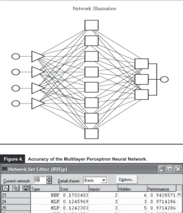
2. Neural Networks Classification with the Multilayer Perceptron Method
The Multilayer Perceptron method with the back propaga-tion activapropaga-tion funcpropaga-tion is a current method of classificapropaga-tion used by the Neural Networks and it is probably one of the most popular and most extensively used (Haykin, 1994, Bishop, 1995, Picon, Varela, Lévy Mangin 2004) in Social Sciences, particularly in marketing. We will use this me-thod to classify the output units using the Statistica Neural Networks program, which selects automatically the best network among many.
The inner units or inputs (4) go into an activation unit through a transfer function to produce an output (3). The number of inputs (here the Petal length, the Petal width, the Sepal length and the Sepal width) and output units (here setosa, virginica and versicolor) is defined by the problem. The number of cases assigned to the training process is 80 over 150 cases. The number of hidden layers (one with 8 intermediate units) has been selected in order to minimize
the prediction error.
The output of each node of the intermediate layer should be estimated by the next function where
n−1 i=0Wij Xi
ϕ
Zj =
ϕ represents the node transfer function, Wij the weights between nodes i and j, Xi the inner units or input and Zj is the exit of the j node. The difference between the node input and the output exit is the error. In our case, a network of 1 hidden layer has generated the best solution with 8 units, as summarized in figure 3.
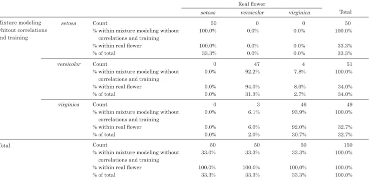
As shown in figure 4, the error training for this network is 0.002442, for the verification set 0.1003 and the global performance is 0.9857143; which is very good.
Figure 1. Mixture modeling with training data and all correlations.
In order to allow training, the data set specifi es that some species data have been a priori defi ned, 10
for setosa (1), 10 for versicolor (2) and 10 for virginica (3).
Figure 2. Latent structure without correlation and no training.
Petal Sepal Mixture Modeling without Correlation and Training
Petal Length Petal Width
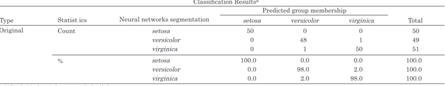
The Multilayer Perceptron Neural network was the most accurate method; it made just 1 error classifying 1 flower ver-sicolor in the virginica species (see table 5A in appendix).
The classification result (see table 6A in appendix) shows that one flower has been wrongly classified virginica when it
is a priori a versicolor species.
The discriminant analysis classifies in base to the original variables (no reference is made to the a priori classification of species) and this classification shows that two errors have been made; one prediction error: one predicted versicolor ori -ginally classified virginica and another one predicted virginica
which has been originally classified versicolor).
3. Traditional Clustering Methods
3.1. K-means Classification Method
The K-means clustering method is a traditional method that reassigns cases by moving them to the cluster whose centroid is the closest to that case. Reassignment continues until every case is assigned to the cluster with the nearest centroid; such a procedure minimizes the variance within each cluster (Har-tigan, J, 1975, Kaufman, L and Rousseuw, P, J, 1990).
This method is very close to Latent Structure Classification or to Classification with Mixture Modeling because both methods optimize some kind of criteria (Log Likelihood or
Intra-class variance) for determining the proximity of cases
to centroids and assign them to the closest group.
The K-means classification is less flexible in relation with the observed variables, in this case variables are mainly metric when the working variables used in Latent Method could be frequencies, ordinal, categorical or metrics or a combination of them. The latent solution is invariant to variables” trans-formation, so they do not need to be standardize.
The K-means method uses distance measures to compute determinist finite classes when the Latent Structure works with post hoc probabilities to compute more fuzzy classes based on Maximum Likelihood Methods (Lévy Mangin, Picon, 2006, 2004).
Table 7A (see appendix) summarizes the classification between K-means clustering method and the real flower a priori classification. This technique does not use any kind of training to classify data as the precedent techniques do; the
results are much more erratic and there is some confusion
in classifying 24 kinds of species predicted versicolor when they originally are virginica species.
The K-means clustering method (see table 8A in appendix) had some problems finding the real virginica classification; discriminant analysis only summarizes 26 a priori cases for this
species if we compare with the real flower classification.
3.2. Hierarchical Classification Method
The Hierarchical method is also a traditional method based (in this case) on Euclidean distance between observations; we
choose it as another reference method and, for comparison
with the less traditional techniques.
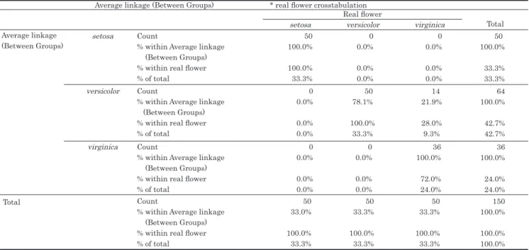
The aggregation technique chosen is Average Linkage. Table 9A (see appendix) shows that setosa species have been perfectly classified (50, 100%), but it found 64 versicolor species instead 50
(128%), and 36 instead 50 virginica (which represents 72%). The discriminant classification matrix (see table 10A in appendix) shows a poor classification in relation with the original flower species; which is satisfactory if we do not compare with a prior probability.
4. Discussion
Section 5 will discuss about the accuracy of all analyzed methods, we will compare methods using objective criteria of analysis as data training, Bayesian estimation and more classical methods, which, do not use these criteria. We will measure the classification (or posterior classification in comparison with the a priori or the
original objective classification) results in relation with the a priori classification and we will make an overall estimation of the method based on specific criteria.
Figure 4. Accuracy of the Multilayer Perceptron Neural Network.
and Training Data. In case of the availability of a previous a priori classification we do not suggest to consider the classical methods of classification (methods 4 and 5, table 12A).
5. Conclusion
Table 12 suggests that the best three methods for classi-fying data consider any form of data training or Bayesian estimation for the posterior classification. The traditional methods perform very poorly in relation with the a priori classification; the classical classification methods are simply less interesting (see table 12A in appendix) when a prior classification of data is made.
Models of Mixture modeling and Latent Structure analysis perform really well and are superior to Neural Networks when it comes to classify into groups with a minimum training of data; these methods are particularly interesting in the case of probabilistic or fuzzy classifications. These methods also permit to identify well-structured groups and an observation does not need to pertain exclusively to just one specific group. This corresponds to what Lilien and Rangaswamy said in 1998 to the effect that the consumer”s segments should be discrete (one consumer in one segment), overlapped (a consumer could pertain to two or more segments), or fuzzy (by assigning a probability to the consumer of pertaining to each group or cluster). To assign a consumer to an exclusive group is more attractive but overlapped and fuzzy segments are more realistic and theoretically and practically more precise.
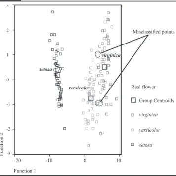
The a priori or original classification is not the perfect classi-fication that everyone could suppose; based on a discriminant analysis classification three species have not been accurately classified. As we can see in table 11A (see appendix), two
versicolor species have been classified as virginica species and one virginica species as versicolor species.
These three misclassified species could easily be observed in figure 5.
The final analysis of each method will be made first, in
relation to the a priori (original) classification, and in a second stage based on the discriminant classification of cases (see table 12A in appendix). We will take in account that some methods have trained the data and others did not. The clas-sification with Multilayer Perceptron trained 80 data over 150, the classification with Mixture Modeling 30 over 150, and all the other methods did not trained any data at all. The classification with Latent Class Mixture Modeling method did not trained any data but it is based on Bayesian Estimation, this method could be shown as one of the most accurate.
- The evaluation of each method based on a cross-tabula-tion between the classificacross-tabula-tion method and the a priori clas -sification shows that the most precise method is the method based on Neural Networks (Classification with Multilayer Perceptron); this method has been extensively trained in comparison with the classification with Mixture Modeling. The other methods have not been trained at all.
The classification with Multilayer Perceptron is not based on a Bayesian Estimation and does not compute an a pos-teriori probability of pertaining to one class in comparison with the two Bayesian methods of classification.
The classical methods are less interesting when an a priori classification is available, tables 8 and 10 suggest that versicolor
and virginica species have been particularly misclassified. - The classification of each method based on discrimi-nant analysis suggests a better classification for the classical methods because there is not an a priori classification. The classification is made based on each method particularities. Nevertheless the methods based on Data Training and on Bayesian Estimation also suggest a very good classification of data (see tables 2A, 4A and 6A).
- As a global evaluation it would be very particularly accu-rate to choose the classification method based on the Neural Networks classification (Multilayer Perceptron), but there is a major inconvenient to generalize results, is that the training data sample is generally most important and extensive than for other methods (Bayesian methods for example). For that reason we cannot assign to this method (in our opinion) the first and an exclusive choice but we can consider it as one of the best. Our first choice will be the classification with Mixture Modeling
Anderson, E. (1935). “The Irises of the Gaspe Peninsula”, Bulletin of the American Iris
Society, 59.
Bishop, C. M. (1995). “Neural Networks for Pattern Recognition”. Oxford University Press, Oxford, United Kingdom.
Ding, C. (2006). “Using Regression Mixture Analysis in Educational Research”. Prac-tical Assessment Research and Evaluation,
11(11).
Hartigan, J. (1975). Clustering Algorithms. John Wiley, New-York. usa.
Haykin, S. I. (1994). Neural Networks: a
Comprehensive Foundation. Mac-Millan,
New-York,usa.
Hoschino, T. (2001). ‘‘Bayesian Inference for Finite Mixtures in Confirmatory Factor Analysis”. Behaviormetrica, 28(1). Kaufmann, L. & P. J. Rousseeuw (1990). Finding
Groups in Data. John Wiley, New-York. usa.
Lazarfeld, P. F. & N. W. Henry (1968). “Latent Structure Analysis”. Houghton-Mifflin Co, Boston, Massachusetts, usa.
Lilien, G. L. & A. Rangaswamy (1998). Mar-keting Management and Strategy: MarMar-keting
Engineering Applications. Prentice-Hall,
New-York, usa.
Lee, S. Y. (2007). Structural Equation Modeling: a Bayesian Approach. John Wiley and sons,
Chichester, uk.
Lévy Mangin, J. P. (2003). Análisis Multivariable
para las Ciencias Sociales. Prentice Hall, Madrid.
Lévy Mangin, J. P. & J. Varela Mallou (2006). “Modelizacion con estructuras de covarian-zas, temas esenciales, avanzados y aportacio-nes especiales”, Netbiblo, Coruña, Spain. Loken, E. (2004). “Using Latent Class Analysis
to Model Temperament Types”. Multivariate Behavioral Research, 39(4).
Magidson, J. (2004). “Latent Class Models. The Sage Handbook of Quantitative Methodo-logy for the Social Sciences”. Thousand Oaks. Sage, California.
Muthen, B. O. (2002). “Beyond sem: General Latent
Variable Modeling”. Behaviormetrica, 29.
Picon-Prado, E.; L. J. & L. M. Varela Mallou (2004). Segmentación de Mercados: Aspectos estratégicos y metodológicos. Prentice-Hall y Financial Times,Madrid.
Vermunt, J. K. & J. Magidson (2002). Latent
Class Cluster Analysis; Applied Latent class Analysis. University Press, Cambridge, Massachusetts.
Vermunt, J. K. & J. Magidson (2002). “Latent-Gold 2 User’s Guide”. Belmont, Massachu-setts: Statistical Innovations.
Vermunt, J. K. & J. Magidson (2005). “Struc-tural Equation Models; Mixture Model”,
Encyclopedia of Statistics in Behavioral
Sciences. John Wiley and Sons, United Kingdom.
Wedel, M. & W. Kamakura (1998). Market Seg-mentation. Conceptual and Methodological
Foundations. Klewer Academics, Boston, Massachussets, usa.
Zhu, H. T. & S. Y. Lee (2001). “A Bayesian Analysis of Finite Mixtures in the Lisrel Model”. Psychometrica, 66(1).
Table 1A. Cross tabulation of mixture modeling with correlation and training with real fl ower.
Mixture modeling whit correlations and training setosa versicolor virginica Total Total
setosa versicolor virginica Real fl ower
Count
% within mixture modeling with
correlations and training
% within real fl ower
% of total Count
% within mixture modeling with
correlations and training
% within real fl ower
% of total Count
% within mixture modeling with
correlations and training
% within real fl ower
% of total Count
% within mixture modeling with
correlations and training
% within real fl ower
% of total 50 100.0% 100.0% 33.3% 0 0.0% 0.0% 0.0% 0 0.0% 0.0% 0.0% 50 33.0% 100.0% 33.3% 0 0.0% 0.0% 0.0% 46 97.9% 92.0% 30.7% 4 7.5% 8.0% 2.7% 50 33.3% 100.0% 33.3% 0 0.0% 0.0% 0.0% 1 2.1% 2.0% 0.7% 49 92.5% 98.0% 32.7% 50 33.3% 100.0% 33.3% 50 100.0% 33.3% 33.3% 47 100.0% 31.3% 31.3% 53 100.0% 35.3% 35.3% 150 100.0% 100.0% 100.0% Appendix Bibliografía
Table 2A. Mixture Modeling with correlation and training. Discriminant analysis classifi cation matrix.
Original
a. 98.7% of original grouped cases correctly classifi ed
Count
%
Total
setosa versicolor virginica Predicted group membership Classifi cation resultsa
setosa versicolor virginica setosa versicolor virginica Mixture modeling with
correlations and training
50 0 0 100.0 0.0 0.0 0 47 2 0.0 100.0 3.8 0 0 51 0.0 0.0 96.2 50 47 53 100.0 100.0 100.0
Table 3A. Cross tabulation of Mixture Modeling without correlation and no training with Real Flower.
Mixture modeling whitout correlations and training setosa versicolor virginica Total Total
setosa versicolor virginica Real fl ower
Count
% within mixture modeling without
correlations and training
% within real fl ower
% of total Count
% within mixture modeling without
correlations and training
% within real fl ower
% of total Count
% within mixture modeling without
correlations and training
% within real fl ower
% of total Count
% within mixture modeling without
correlations and training
% within real fl ower
% of total 50 100.0% 100.0% 33.3% 0 0.0% 0.0% 0.0% 0 0.0% 0.0% 0.0% 50 33.0% 100.0% 33.3% 0 0.0% 0.0% 0.0% 47 92.2% 94.0% 31.3% 3 6.1% 6.0% 2.0% 50 33.3% 100.0% 33.3% 0 0.0% 0.0% 0.0% 4 7.8% 8.0% 2.7% 46 93.9% 92.0% 30.7% 50 33.3% 100.0% 33.3% 50 100.0% 33.3% 33.3% 51 100.0% 34.0% 34.0% 49 100.0% 32.7% 32.7% 150 100.0% 100.0% 100.0%
Table 4A. Mixture Modeling without correlation and no training; Discriminant analysis classifi cation matrix.
Original
a. 99.3% of original grouped cases correctly classifi ed. Count
%
Total
setosa versicolor virginica Predicted group membership Classifi cation resultsa
setosa versicolor virginica setosa versicolor virginica Mixture modeling without
correlations and training
50 0 0 100.0 0.0 0.0 0 51 1 0.0 100.0 2.0 0 0 48 0.0 0.0 98.0 50 51 49 100.0 100.0 100.0
Table 5A. Cross tabulation of the Multilayer Perceptron Neural Networks classifi cation with correlation and training with Real Flower. (Begins)
Neural networks
segmentation setosa
Total
setosa versicolor virginica Real fl ower
Count
% within neural networks
segmentation % within real fl ower
% of total 50 100.0% 100.0% 33.3% 0 0.0% 0.0% 0.0% 0 0.0% 0.0% 0.0% 50 100.0% 33.3% 33.3%
Table 6A. Neural Networks discriminant analysis classifi cation matrix.
Original
a. 96.7% of original grouped cases correctly classifi ed.
Count Statist ics
Type
%
Total
setosa versicolor virginica Predicted group membership Classifi cation Resultsa
setosa versicolor virginica setosa versicolor virginica
Neural networks segmentation
50 0 0 100.0 0.0 0.0 0 48 1 0.0 98.0 2.0 0 1 50 0.0 2.0 98.0 50 49 51 100.0 100.0 100.0
Table 7A. Cross tabulation of K-Means classifi cation with Real Flower.
Qmeans clustering setosa versicolor virginica Total Total
setosa versicolor virginicaReal fl ower
Count
% within Qmeans clustering % within real fl ower
% of total Count
% within Qmeans clustering % within real fl ower
% of total Count
% within Qmeans clustering % within real fl ower
% of total Count
% within Qmeans clustering % within real fl ower
% of total 50 100.0% 100.0% 33.3% 0 0.0% 0.0% 0.0% 0 0.0% 0.0% 0.0% 50 33.3% 100.0% 33.3% 0 0.0% 0.0% 0.0% 50 67.6% 100.0% 33.3% 1 2.0% 2.0% 0.7% 50 33.3% 100.0% 33.3% 0 0.0% 0.0% 0.0% 24 32.4% 48.0% 16 .0% 26 100.0% 52.0% 17.3% 50 33.3% 100.0% 33.3% 50 100.0% 33.3% 33.3% 74 100.0% 49.3% 49.3% 26 100.0% 17.3% 17.3% 150 100.0% 100.0% 100.0%
Table 8A. Discriminant Classifi cation matrix for K-Means clustering method.
Original
a 95.3% of original grouped cases correctly classifi ed. Count
%
Total
setosa versicolor virginica Predicted group membership Classifi cation Resultsa
setosa versicolor virginica setosa versicolor virginica Qmeans clustering 50 0 0 100.0 0.0 0.0 0 67 0 0.0 90.5 0.0 0 7 26 0.0 9.5 100.0 50 74 26 100.0 100.0 100.0
Table 5A. Cross tabulation of the Multilayer Perceptron Neural Networks classifi cation with correlation and training with Real Flower. (Concludes)
Neural networks
segmentation
Total
setosa versicolor virginicaReal fl ower versicolor
virginica
Total
Count
% within neural networks
segmentation % within real fl ower
% of total Count
% within neural networks
segmentation % within real fl ower
% of total Count
% within neural networks
segmentation % within real fl ower
% of total 0 0.0% 0.0% 0.0% 0 0.0% 0.0% 0.0% 50 33.0% 100.0% 33.3% 49 100.0% 98.0% 32.7% 1 2.0% 2.0% 0.7% 50 33.3% 100.0% 33.3% 0 0.0% 0.0% 0.0% 50 98.0% 100.0% 33.3% 50 33.3% 100.0% 33.3% 49 100.0% 32.7% 32.7% 51 100.0% 34.0% 34.0% 150 100.0% 100.0% 100.0%
Table 9A. Cross tabulation of the Multilayer Perceptron Neural Networks classifi cation with correlation and training with Real Flower.
Average linkage
(Between Groups) setosa
versicolor
virginica
Total
Total
setosa versicolor virginica Real fl ower
Average linkage (Between Groups) * real fl ower crosstabulation
Count
% within Average linkage (Between Groups) % within real fl ower
% of total Count
% within Average linkage (Between Groups) % within real fl ower
% of total Count
% within Average linkage (Between Groups) % within real fl ower
% of total Count
% within Average linkage (Between Groups) % within real fl ower
% of total 50 100.0% 100.0% 33.3% 0 0.0% 0.0% 0.0% 0 0.0% 0.0% 0.0% 0 0.0% 0.0% 0.0% 50 33.0% 100.0% 33.3% 0 0.0% 0.0% 0.0% 50 78.1% 100.0% 33.3% 50 33.3% 100.0% 33.3% 0 0.0% 0.0% 0.0% 14 21.9% 28.0% 9.3% 36 100.0% 72.0% 24.0% 50 33.3% 100.0% 33.3% 50 100.0% 33.3% 33.3% 64 100.0% 42.7% 42.7% 36 100.0% 24.0% 24.0% 150 100.0% 100.0% 100.0%
Table 10A. Discriminant Classifi cation matrix for K-Means clustering method.
Original
a. 96.7% of original grouped cases correctly classifi ed. Count
%
Total
setosa versicolor virginicaPredicted group membership Classifi cation resultsa
setosa versicolor virginica setosa versicolor virginica
Average linkage (Between Groups)
50 0 0 100.0 0.0 0.0 0 59 0 0.0 92.2 0.0 0 5 36 0.0 7.8 100.0 50 64 36 100.0 100.0 100.0
Table 11A. Discriminant Classifi cation matrix for original classifi cation method.
Original
a 98,0% of original grouped cases correctly classifi ed. Count
%
Total
setosa versicolor virginicaPredicted group membership
setosa versicolor virginica setosa versicolor virginica Real fl ower 50 0 0 100.0 0.0 0.0 0 48 1 0.0 96.0 2.0 0 5 36 0.0 4.0 98.0 50 64 36 100.0 100.0 100.0 Classifi cation resultsa
Table 12A. Comparing performance of each classifi cation method.
Method of Classifi cation
Mixture Modeling and training data Yes No Yes No No Yes Yes No No No Very Satisfactory (2nd classifi ed) Very Satisfactory (3rd classified) Excellent (1rst classified) Very Satisfactory (3rd classifi ed) Very Satisfactory (2nd classified) Excellent (2nd classified) Very Satisfactory
(1rst classifi ed) Very Satisfactory(1rst classifi ed)
Excellent (3rdclassifi ed) Very Satisfactory (5nd classifi ed) Very Satisfactory (5nd classifi ed) Excellent (5nd classifi ed) Very Satisfactory (4nd classifi ed) Very Satisfactory (4nd classifi ed) Excellent (4nd classifi ed)
Latent Structure Analysis Multilayer Perceptron
Hierarchical method K-means
Bayesian Estimation
Accuracy of the Discriminant Analysis Results2 (Classifi cation)
Data
Training
Accuracy of Classifi cation
Results1 (Crosstabulation)
Overall evaluation of the method and choice
1 Posterior classifi cation in relation with a priori fl ower species classifi cation (method based on cross-tabulation with original data).