HIGH PRECISION TIMING
Dissertation
zur
Erlangung des Doktorgrades (
Dr. rer. nat.
)
der
Mathematisch–Naturwissenschaftlichen Fakultät
der
Rheinische Friedrich–Wilhelms–Universität Bonn
vorgelegt von
Eleni Graikou
aus
Katerini, Griechenland
1. Referent: Prof. Dr. Michael Kramer
2. Referent: Prof. Dr. Norbert Langer
Tag der Promotion: 19.12.2018
Erscheinungsjahr: 2019
Diese Dissertation ist auf dem Hochschulschriftenserver der ULB Bonn unter
RHEINISCHEN FRIEDRICH–WILHELMS–UNIVERSITÄT BONN
Abstract
of the dissertation: “High precision timing”
by Eleni Graikou
for the degree of
Doctor rerum naturalium
Pulsars are highly magnetised, fast spinning neutron stars (NSs), formed after a supernova explosion. The core of their progenitor star, which is around 1–2 M⊙, is compressed to a radius of only∼10 km, making them one of the most compact objects observed. From each magnetic pole a highly magnetised beam of electromagnetic radiation is emitted, the exact emission mechanism of which is not yet fully understood. Since the magnetic axis is generally not aligned with the spin axis, the emission beam sweeps across the sky. In the cases that the emission beam crosses the line of sight of the telescope, once every rotation we detect a pulse of radiation.
The majority of science that we can do with pulsars comes from pulsar timing. With timing we compare the observed pulse arrival times to a model that contains the rotational, astrometric, interstellar medium (ISM) related, and binary (if the pulsar belongs to a binary system) properties of the pulsar. The goal is to create a model that correctly described the behaviour of the pulsar. Millisecond pulsars (MSPs), which are pulsars with spin periods of only a few milliseconds, are the ideal objects to apply timing, since their rotational stability on long timescales approaches that of atomic clocks.
Probably one of the most interesting applications of pulsar timing is the detection of grav-itational waves (GWs) in the nHz regime. Main sources of these low frequency GWs are inspiraling super-massive black hole binaries (SMBHBs). GW signal can be from individual sources or from the gravitational wave background (GWB) made from the superposition of the cosmic population of the SMBHBs. A GW signal can be detected as a correlated red noise signal in the timing residuals of a pulsar timing array (PTA), formed by timing stable MSPs, almost homogeneously distributed on the sky. Since the GW signal is very weak, in order to make a detection, a timing stability of around 100 ns over a timescale of 5 years is required for PTA pulsars. The main source of red noise in pulsars that should be modeled, for achiev-ing this high timachiev-ing precision, is chromatic variations produced by perturbations on the ISM. In Chapter3 we investigate the usage of Effelsberg and MeerKAT high-frequency receivers (both those presently used and those being commissioned) for measuring DM variations and increasing the PTA sensitivity to continuous GWs and GWBs. Six years of Effelsberg EPTA observations at 1.4 and 2.6 GHz are reviewed in this chapter, the performance of which is used to select the sources that will be observed at 4.8 GHz. 14 pulsars have been detected at these high frequencies: for the seven with the longest data set we further reported signal-to-noise ratio values, flux density measurements, and DM variation measurements. We discuss the potential of complementing the existing EPTA data set with receivers that are now in a com-missioning stage. We concluded that the combination of Effelsberg 1.4 GHz and MeerKAT S-band observations, for flux density spectral indices≲−1.6, provides the best precision for
measuring DM variations existing from the 21 cm and the 11 cm receiver, an addition of 6.7 years for a GWB and another 80 years of observations for continuous GWs, on the top of 10, are needed in order to achieve the same sensitivity as we expect for the Effelsberg 21-cm combined with MeerKAT 11-cm observations.
In Chapter4, we performed timing analysis of the PSR J1933−6211, a 3.5-ms pulsar with a WD companion. The observations used in the analysis were conducting with the Parkes radio telescope in Australia. The goal of this project was to reveal the nature of the WD companion. Based on scintillation and timing analysis we concluded that the pulsar has, as have very few other fully recycled MSPs, a CO companion. The formation of this system can be explained with an intermediate-mass X-ray binary. In this case the transfer of masses started when the WD companion was still in main sequence stage and thus the transfer of mass through a Roche-lobe overflow lasted long enough time scale to fully recycle the pulsar.
In Chapter5the relativistic effect, geodetic precession is studied in PSR B1913+16. This effect has as a result the spin axis to precessing about the total angular momentum axis. This causes the line of sight to cut different parts of the emission beam through time, making the total intensity profile and the polarisation properties to gradually change following a peri-odicity of around 300 years (for this pulsar). By studying these variations we can derive the emission geometry of the system. For our analysis we used observations taken with Arecibo and Effelsberg radio telescope at observing wavelength of 21 cm. The effect of geodetic pre-cession on the separation and the relative amplitude of the two main pulse components were obvious. After applying two independent to each other models, one fitted to the total in-tensity and the other to our polarisation data, we concluded that the inclination angle of the PSR B1913+16 system is 132.9◦and the misalignment angle∼21◦, and also that the emission beam is probably hollow-cone with the magnetic axis not being positioned at the center of the beam but shifted around 10◦from the center.
Acknowledgment
This thesis would not be possible without the valuable help of many people that I will
attempt to mention all below.
I would really want to thank Michael Kramer for all the support and help that
he provided me all these years, for reading my thesis very fast and for creating the
Fundamental physics group, in which I was lucky to be a member. This group is an
environment that develops students into scientists, most particular the next
genera-tion of pulsar astronomers.
I would also like to thank my two advisors, David Champion and Joris Verbiest
for all the support, encouragement, and guidance that they gave me all these years.
Despite their very busy schedules, they always found time to answer all my questions
and tolerated my mistakes. They were my motivation that kept pushing me further,
without their help my PhD would not be completed.
Besides my advisors, I would like to thank all the members of the fundi group
that are very willing to share their knowledge about pulsars and for creating a fun
working environment. I want to particularly mention Greeegoryyy Desvignes, Paulo
Freire, Ramesh Karuppusamy, Axel Jessner, and Stefan Osłowski. Also special thanks
to James McKee and Nataliya Porayko who helped in proof-reading part of this thesis.
I am grateful to Kira Kühn and Le Tran for helping me with all the paper work
that I had to do, so that I can only focus on my work.
I also would like to acknowledge the support of the technical staff of Effelsberg.
They really made MANY of my observations a lot easier and in some cases they
helped solved any problem I had right away.
I would also like to thank the officemates that I have had all these years:
Car-olina!, Ancor!, Philip!, Pablo!, Marina!, Alice!, Andrew!, Jason!, and last but not least
Natasha!. She is the best officemate that I could ever ask for. Also, I would like
to thank all the other students of the fundi group for all the scientific discussions,
but also all the fun that we had. I would more particularly mention Cherry!, Mary!,
Tilemachos!, Ale-Ale-Alessandro!, Henning!, Nicolas!, and especially Patrick!. And
other students from the institute Hans!, WonJu!, Fateme!, Maitraiyee!, and Vica!.
A big thanks to my family, my father, my mother, and my sister Georgia. Without
their guidance and support I would not have been able to start a PhD. They motivated
me to pursue my dreams even though that meant that I had to go far away from them.
I want also to thank Joey for all the support that he gave me all these years, and
all the effort that he put for making me a better person.
Last but not least I want to thank my first supervisor John Seiradakis. I am feeling
very lucky that I have worked with him. If it was not for him, I would not be here
today.
Contents
1
Introduction
1
1.1
The discovery of pulsars
. . . .
2
1.2
The nature of pulsars and the emission mechanism
. . . .
3
1.3
Pulsar model
. . . .
4
1.3.1
Spin evolution
. . . .
4
1.3.2
Ages of pulsars
. . . .
6
1.3.3
Magnetic field strength
. . . .
6
1.4
The pulsar population
. . . .
7
1.4.1
Formation of recycled pulsars
. . . .
7
1.5
Observing pulsars
. . . .
11
1.5.1
Integrated profile
. . . .
11
1.5.2
Flux density spectra
. . . .
12
1.5.3
Polarization properties
. . . .
13
1.6
Modeling the radio emission beam
. . . .
14
1.6.1
Rotating-vector model (RVM)
. . . .
14
1.6.2
Radius-to-frequency mapping (RFM)
. . . .
17
1.7
Pulsar beam structure
. . . .
19
1.8
Interstellar medium effects
. . . .
19
1.8.1
Dispersion
. . . .
20
1.8.2
Faraday rotation
. . . .
21
1.8.3
Scattering and scintillation
. . . .
22
1.9
Pulsar applications
. . . .
23
1.9.1
Mass measurements and equation of state
. . . .
23
1.9.2
Binary and stellar evolution
. . . .
24
1.9.3
Tests of gravity theories
. . . .
25
1.9.4
Searching for gravitational waves
. . . .
25
1.9.4.1
PTA experiments
. . . .
26
2
Timing a pulsar
31
2.1
Timing observations
. . . .
32
2.1.1
Frontend
. . . .
32
2.1.2
Backend
. . . .
33
2.1.2.1
Incoherent and coherent de-dispersion
. . . .
33
2.1.2.2
Folding mode
. . . .
35
2.2
Data reduction
. . . .
35
2.2.1
RFI mitigation
. . . .
35
2.2.2
Polarisation calibration
. . . .
36
2.2.3
RM correction
. . . .
38
2.2.4
Flux calibration
. . . .
38
2.3
Timing analysis
. . . .
39
2.3.1
ToA measurement
. . . .
39
2.3.2
Timing model
. . . .
41
2.3.2.1
Barycentric corrections
. . . .
41
2.3.2.2
Interstellar corrections
. . . .
42
2.3.2.3
Binary corrections
. . . .
43
2.3.3
Timing residuals
. . . .
45
2.3.4
Sources of noise
. . . .
46
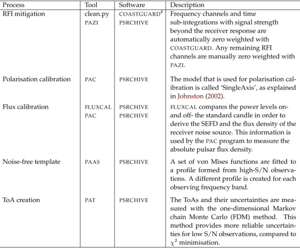
3
Prospects of determining DM variations with Effelsberg multi-frequency
observations
49
3.1
Introduction
. . . .
50
3.2
Observations and data analysis
. . . .
52
3.3
Results
. . . .
56
3.3.1
Flux density and spectral indices measurements
. . . .
56
3.3.2
Comparison of multi-frequency observations
. . . .
60
3.3.2.1
Profile evolution with frequency
. . . .
60
3.3.2.2
ToA uncertainties
. . . .
62
3.3.3
DM time variations
. . . .
65
3.3.4
DM time variations with future receivers
. . . .
65
3.4
Implication for continuous GWs and GWB detection
. . . .
73
3.5
Conclusions
. . . .
75
4
The system parameters of PSR J1933
−
6211
77
4.1
Introduction
. . . .
78
4.2
Observations and data reduction
. . . .
80
4.3
Timing solution and high-precision potential
. . . .
84
4.3.1
Mass constraints from timing
. . . .
85
4.3.2
Characteristic age
. . . .
85
4.4
Scintillation measurements
. . . .
86
4.4.1
Transverse velocity and inclination angle limit
. . . .
87
4.5
Limits on the system masses
. . . .
89
Contents
v
4.5.2
Orbital period – WD mass relation
. . . .
90
4.6
Conclusions
. . . .
92
5
The beam geometry of PSR B1913+16
93
5.1
Introduction
. . . .
94
5.2
Observations and data reduction
. . . .
96
5.2.1
EPOS observations
. . . .
96
5.2.2
PSRIX observations
. . . .
97
5.2.2.1
Polarisation and flux calibration
. . . .
97
5.2.3
Rotation measure
. . . .
98
5.3
Results
. . . .
98
5.3.1
Beam geometry based on total intensity analysis
. . . .
98
5.3.1.1
Relative amplitude changes
. . . 101
5.3.1.2
Profile width changes
. . . 101
5.3.1.3
Component separation changes
. . . 101
5.3.2
Emission beam geometry based on polarisation analysis
. . . . 106
5.3.2.1
Polarisation properties
. . . 106
5.3.2.2
RVM fitting
. . . 106
5.3.2.3
Comparison of solutions
. . . 109
5.3.3
Beam shape
. . . 114
5.4
Conclusions
. . . 118
6
Conclusions
119
Bibliography
123
List of Figures
1.1
A simplified pulsar model.
. . . .
5
1.2
The period–period derivative diagram (
P
–
P
˙
diagram).
. . . .
8
1.3
Two paths to form a recycled NS.
. . . .
10
1.4
Geometry of the pulsar emission beam.
. . . .
15
1.5
Different examples of PPA as a function of pulse phase.
. . . .
16
1.6
Hellings and Downs curve.
. . . .
27
2.1
The effect of dispersion on a pulsar observation.
. . . .
34
2.2
An example of pulsar observation affected by RFI.
. . . .
37
3.1
The galactic distribution of EPTA pulsars, regularly observed with the
Effelsberg radio telescope at 1.4 GHz, and the subset of these pulsars
that are also monitoring at 4.85 GHz.
. . . .
52
3.2
SEFD measurements of the receivers used for EPTA observations based
on quasar observations.
. . . .
55
3.3
Flux density measurements of 33 pulsars at 1.4 GHz with PSRIX.
. . .
59
3.4
Flux density spectra for seven EPTA pulsars from
∼
100 MHz to 4.85 GHz.
61
3.5
Multi-frequency noise-free templates for the PSRs J1643
−
1224 and
J1744
−
1134, in which no significant changes on the shape or in the
pro-file width have been observed on the PSRIX Effelsberg observations.
.
62
3.6
Multi-frequency noise-free templates for the PSRs J1600
−
3053,
J1713+0747, J1730
−
2304, J1857+0943 and J1939+2134, in which
signifi-cant changes on the shape or in the profile width have been observed
on the PSRIX Effelsberg observations.
. . . .
63
3.7
Profile width measurements at 10% intensity level of seven pulsars
based on PSRIX Effelsberg observations.
. . . .
64
3.8
Profile width measurements at 50% intensity level of seven pulsars
based on PSRIX Effelsberg observations.
. . . .
64
3.9
DM variations as a function of time for seven EPTA pulsars.
. . . .
66
3.10 Expected ToA uncertainties of the existing and future Effelsberg
re-ceivers as a function of pulsar flux density spectral index.
. . . .
68
3.11 Comparison of the theoretical expected and the observable ToA
uncer-tainty of observations with the Effelsberg ‘S110 mm’ and ‘S60 mm’
re-ceivers scaled to ‘P217 mm’ values, as a function of pulsar flux density
spectral index.
. . . .
69
3.12 Simulated DM variations as a function of time for seven EPTA pulsars.
70
3.13 The precision that we can achieve in DM variation measurements as a
function of flux spectral index, based on simulated data.
. . . .
71
3.14 Distribution of published pulsar flux density spectral indices.
. . . . .
72
3.16 Sensitivity curves to continuous GWs.
. . . .
74
4.1
The position of PSR J1933
−
6211 in the period - period derivative diagram
79
4.2
Average polarization calibrated pulse profile of PSR J1933
−
6211 at 1382
MHz central frequency
. . . .
82
4.3
The timing residuals of PSR J1933
−
6211, at 20 cm as a function of
or-bital phase
. . . .
84
4.4
Mass – inclination angle diagram of PSR J1933
−
6211 based on timing
.
86
4.5
Dynamic spectrum of a full scintle of PSR J1933
−
6211
. . . .
88
4.6
Pulsar mass – companion mass diagram of PSR J1933
−
6211
. . . .
90
4.7
PSR J1933
−
6211 mass estimate as a function of inclination angle
. . . .
91
5.1
The rotation measure of the PSRIX B1913+16 obervations.
. . . .
99
5.2
Total intensity PSR B1913+16 pulse profiles as a function of time.
. . . 100
5.3
The amplitude ratio of the leading and trailing components pf
PSR B1913+16 as a function of time.
. . . 102
5.4
The width of the whole pulse profile of PSR B1913+16 as a function of
time, at seven different intensity levels.
. . . 103
5.5
The phase-averaged flux densities of PSRIX PSR B1913+16
observa-tions as a function of time.
. . . 104
5.6
Separation of the two main pulse components of PSR B1913+16 as a
function of time.
. . . 105
5.7
One and two dimensional projections of the posterior probability
distributions for the five parameters of the total intensity model of
PSR B1913+16.
. . . 107
5.8
Average percentage of linear (top) and circular polarisation (bottom),
based on our PSRIX PSR B1913+16 observations, as a function of time.
108
5.9
The averaged polarisation profiles and the PPA measurements of
PSR B1913+16 at 10 different epochs.
. . . 110
5.9
The averaged polarisation profiles and the PPA measurements of
PSR B1913+16 at 10 different epochs.
. . . 111
5.10 All the PPA measurements of PSR B1913+16 as a function of pulse
phase based on PSRIX observations.
. . . 112
5.11 One and two dimensional projections of the posterior probability
List of Figures
ix
5.12 The prediction of the evolution of the impact parameter of
PSR B1913+16 as a function of time for
i
=47.1
◦.
. . . 115
5.13 The prediction of the evolution of the impact parameter of
PSR B1913+16 as a function of time for
i
=132.9
◦.
. . . 116
5.14 Comparison of the geometrical model and RVM predictions on
PSR B1913+16 line of sight changes through time.
. . . 116
5.15 A proposed emission beam model for the PSR B1913+16.
. . . 117
List of Tables
3.1
The technical characteristics of systems used for the Effelsberg EPTA
observations.
. . . .
53
3.2
List of softwares used in this chapter for cleaning, polarisation and flux
calibration, and creating ToAs.
. . . .
54
3.3
Phase-averaged flux density measurements of 33 EPTA pulsars with
the Effelsberg radio telescope at 1.4 GHz.
. . . .
57
3.4
Flux density measurements of seven EPTA pulsars with the Effelsberg
radio telescope at 2.6 GHz.
. . . .
58
3.5
Flux density measurements of seven EPTA pulsars with the Effelsberg
radio telescope at 4.85 GHz.
. . . .
58
3.6
Spectral indices of seven EPTA pulsars based on Effelsberg PSRIX
ob-servations and previously published flux densities.
. . . .
60
3.7
The median ToA uncertainties, all referring to 28-min integration time,
of seven pulsars at 1.4, 2.6 and 4.85 GHz with PSRIX back-end.
. . . . .
65
3.8
The technical characteristics of future systems planned to be used for
pulsar observations.
. . . .
67
4.1
The timing data characteristics of PSR J1933
−
6211, as observed with
CPSR2 and CASPSR
. . . .
81
4.2
The timing parameters of PSR J1933
−
6211
. . . .
83
4.3
Scintillation parameters and the derived scintillation speed based on
scintles of PSR J1933
−
6211
. . . .
87
4.4
PSR J1933
−
6211 pulsar’s WD companion mass estimates assuming
dif-ferent chemical compositions of its progenitor star
. . . .
91
5.1
Geometrical model solutions with 1-
σ
uncertainties.
. . . 106
5.2
RVM solutions with 1-
σ
uncertainties.
. . . 109
Frequently Used Symbols
ADC Analogue-to-Digital Converters BAT Barycentric arrival time
BB Binary system barycentre BH Black hole
BIPM Bureau International des Poids et Mesures
BMSP Binary millisecond pulsars CPSR2 Caltech Swinburne
Parkes Recorder 2 CE Common envelope
CHIME Canadian Hydrogen Intensity Mapping Experiment
CO Carbon-oxygen
CO WD Carbon-oxygen white dwarf DM Dispersion measure
DNS Double neutron star EoS Equation of state
EPTA European pulsar timing array FAST Five-hundred-meter Aperture
Spherical radio Telescope FFT Fast Fourier Transform GR General relativity GW Gravitational wave
GWB Gravitational wave background He GW Helium white dwarf
HMXB High-mass X-ray binary
IMXB Intermediate-mass X-ray binary IPTA International pulsar timing array ISM Interstellar medium
JPL Jet Propulsion Laboratory LIGO Gravitational-Wave Observatory LISA Laser Interferometer Space Antenna LMXB Low-mass X-ray binary
LNA Low-Noise Amplifier LOFAR Low-Frequency Array MCMC Markov-chain Monte-Carlo MJD Modified Julian Dates MS Main sequence
MSP Millisecond pulsar
NANOGrav North American Nanohertz
Observatory for gravitational waves NIST National Institute of Standard
and Technology
NS Neutron star
OMT Ortho-mode Transducers ONeMg Oxygen-neon-magnesium ONeMg WD Oxygen-neon-magnesium
white dwarf
PFB Polyphase filter-bank PK Post-Keplerian
PPA Polarisation position angle PPTA Parkes pulsar timing array PTA Pulsar timing array
RFI Radio frequency interference RFM Radius-to-frequency mapping RLO Roche-lobe overflow
RM Rotation measure RMS Root-mean-square
timing residuals RVM Rotating-vector model SAT Site arrival times
SEP Strong equivalent principle SKA Square Kilometre Array SSB Solar System barycentre SSE Solar System ephemeris SMBH Super-massive black hole SMBHB Super-massive black hole binary S/N Signal-to-noise ratio
SN Supernova
SSB Solar System barycenter TAI International Atomic Time TCB Barycentric Coordinate Time ToA Time of arrival
TT Terrestrial time
UTC Universal Coordinated Time VLBI Very-Long-Baseline Interferometry
Chapter
1
Introduction
Contents
1.1 The discovery of pulsars. . . . 2
1.2 The nature of pulsars and the emission mechanism . . . . 3
1.3 Pulsar model . . . . 4
1.3.1 Spin evolution. . . 4
1.3.2 Ages of pulsars . . . 6
1.3.3 Magnetic field strength . . . 6
1.4 The pulsar population . . . . 7
1.4.1 Formation of recycled pulsars. . . 7
1.5 Observing pulsars . . . . 11
1.5.1 Integrated profile . . . 11
1.5.2 Flux density spectra . . . 12
1.5.3 Polarization properties. . . 13
1.6 Modeling the radio emission beam . . . . 14
1.6.1 Rotating-vector model (RVM) . . . 14
1.6.2 Radius-to-frequency mapping (RFM) . . . 17
1.7 Pulsar beam structure . . . . 19
1.8 Interstellar medium effects . . . . 19
1.8.1 Dispersion . . . 20
1.8.2 Faraday rotation . . . 21
1.8.3 Scattering and scintillation . . . 22
1.9 Pulsar applications . . . . 23
1.9.1 Mass measurements and equation of state. . . 23
1.9.2 Binary and stellar evolution . . . 24
1.9.3 Tests of gravity theories . . . 25
1.1
The discovery of pulsars
In 1934, only two years after the discovery of neutrons,Baade & Zwicky(1934) proposed that the outcome of a supernova explosion can be a very compact stellar remnant with density up to 1015g cm−3. The interior would be composed mainly from neutrons. Colgate & White (1966) predicted that the remnant would reach spin frequencies of tens to hundreds of Hz and would have strong magnetic field, due to conservation of magnetic flux and angular momentum. Later, in 1967, only a few months before the discovery of pulsars,Pacini(1967) showed that the strong magnetic field of a spinning neutron star (NS) could result in magnetic dipole emission, energetic enough to energise the surrounding remaining nebula.
Despite the growth of radio astronomy since the 1930’s, more than 30 years passed until the discovery of pulsars. That was partly due to the fact that radio astronomers were not expecting to find rapid period fluctuations in the signals from any celestial source. Indeed, most radio receivers were designed to reject or smooth out impulsive signals and to measure only steady signals, averaged over several seconds of integration time.
The first pulsar was discovered unexpectedly, during a research investigation of the in-terplanetary scintillations carried out by Anthony Hewish and his student Jocelyn Bell at the Mullard Radio Astronomy Observatory in Cambridge. The Interplanetary Scintillation Ar-ray that was used for this research was operating at long radio wavelengths (3.7 m). At this wavelength, radio sources with very small angular diameters are affected by interplanetary scintillation. In July 1967, a month after the beginning of recording, Jocelyn Bell noticed large signal fluctuations coming from a specific location in the sky. When these fluctuations reap-peared at the same sidereal time, there was no doubt that they had celestial origin. A recorder with an even faster response time was used and in November 1967, regular pulses with a period of∼1.337 s were observed.
In February 1968 the discovery of this first pulsar, now known as PSR J1921+2153 (B1919+21), was announced byHewish et al.(1968). In this paper, also, an initial interpre-tation about the nature of this source was presented. Hewish et al. (1968) concluded that the source lies outside the Solar System, since it was appearing at the same sidereal time ev-ery day, the observations did not show any evidence of parallax, and a frequency dispersion withing the 1-MHz band is observed. Also, based on the regularity and the rapidity of the pulsations, they argued that the source must be a radially oscillating condensed star, presum-ably either a white dwarf (WD) or a NS. The term “pulsar” (standing for PULSating stAR) was given to this newly discovered class of objects. By the end of the same year, three more pulsars were discovered with similar properties (Pilkington et al.,1968). In 1974 Hewish was awarded a Nobel prize in physics for this discovery.
The discovery of pulsars triggered a series of observations from all the large radio obser-vatories at the time. By the end of 1968 more than 100 papers either reporting new discoveries or investigating pulsar properties were published. Major efforts were made to understand the nature of pulsars by, for example, observing their polarization properties, performing multi-frequency observations, and investigate their profiles. These observations challenged theoreticians to propose new models to explain the pulsar emission.
Three main mechanisms were proposed to explain the regular pulsed emission from pul-sars: pulsating (Hewish et al.,1968;Burbidge,1968), orbiting (Burbidge,1968;Saslaw,1968), and rotating (Ostriker,1968;Gold,1968) WDs or NSs. The pulsating WD and NS, and rotat-ing WD scenarios were ruled out after the discovery of the Vela (J0835−4510 (B0833-45),Large et al.,1968) and Crab pulsars (J0534+2200 (B0531+21),Staelin & Reifenstein,1968), since they have pulse periods of only∼89 ms and∼33 ms, respectively. According to theoretical models WDs and NSs could oscillate with periods as short as 100 ms, and∼1 s (Thorne & Ipser,1968),
1.2. The nature of pulsars and the emission mechanism
3
respectively. Rotating WDs have also been excluded since for rotation periods of less than a second the centrifugal forces would disrupt their outer layers.
Orbiting WD and NS scenarios ruled out after an decrease in the pulsation rate was ob-served (Davies et al.,1969, and many others since). WD and NS systems should gradually lose orbital energy through gravitational-wave (GW) emission resulting in a gradual decrease of orbital period, which was in contradiction with the observations.
Rotating NSs remained as the only plausible explanation. Following a prediction by Pacini(1967) for the Crab pulsar,Gold(1968) was the first to identify pulsars as rotating NSs. According to his model the very strong magnetic fields, combined with high spin frequencies, result in the creation of an ionized magnetosphere which co-rotates with the NS. When the co-rotation reaches the speed of light, the plasma will escape the magnetosphere creating the emission beam. Furthermore, he predicted a decreasing spin period (due to energy loss in the form of magnetic dipole radiation), the potential existence of faster pulsars, and the asso-ciation between supernova remnants and pulsars (Gold,1969). Observations verified all his predictions. Today, even though the exact emission mechanism is not clear, there is no doubt that pulsars are rotating NSs.
1.2
The nature of pulsars and the emission mechanism
Pulsars are formed during a core-collapse supernova event. Their formation path starts with a massive main sequence (MS) star of around 8 to 15 M⊙(Woosley & Weaver,1986;Carroll & Ostlie,2006). As the star evolves, it fuses increasingly heavy nuclei in its core: H to He; He to C, N, O; C, N, O to Si. Finally, the fusion of the Si core result in the creation of a56
26Fe rich core. The very high temperatures reached during the nuclear fusion, give to the photons enough energy to destroy heavy nucleii; like iron, in protons and neutrons, a process known as photo-disintegration. The fusion of56Fe is an endothermic process, resulting in the removal of thermal energy, and a drop of the core radiation pressure. The electrons that supported, so far, the star from collapsing, are now captured by the atomic nuclei, and the protons that are formed by photo-disintegration. The core, having no process by which to resist gravity, starts collapsing until it reaches the Chandrasekhar mass (≃1.4M⊙). When the density of the inner core exceeds 8×10¹⁴g cm−3, the strong force becomes repulsive, resulting in a rebound of the in-falling matter of the outer layers. The shock wave expels the majority of the star’s mass, leaving behind an ultra-dense core. The energy that is released from an explosion like this can reach values of∼1010L
⊙ (Arnett,1996), equivalent to the brightness of an entire galaxy. This creation scenario can be also verified from the multiple supernova remnants found to be associated with the remaining products of the explosion: pulsars (e.g.Staelin & Reifenstein, 1968;Strom,1987;Frail & Kulkarni,1991).
If the mass of the remaining core is less than the Tolman−Oppenheimer−Volkoff limit (Tolman,1939; Oppenheimer & Volkoff,1939), the collapse of the star is prevented by the neutron degeneracy pressure, leaving a NS behind. In the case where the mass is above this limit, the star is collapses further under the pressure of gravity, creating ablack hole(BH).
NSs are highly magnetized, extremely compact objects. The remaining mass of the pro-genitor star, after the supernova explosion, is around 1−2 M⊙, and is contained within a ra-dius of only∼10 km (Lattimer & Prakash,2001). The density of the star’s interior is 6.7×10¹⁴g cm−3, comparable to nuclear density. The exact structure in the interior can be determined from the equation of state (EoS). Unfortunately, the EoS for NSs is still unclear, which pre-vents us from knowing their basic physical properties, like the interior mass or the radius (see Section1.9.1).
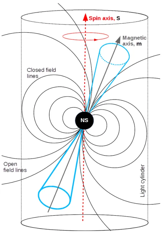
Pulsars are a subcategory of NSs. Due to conservation of angular momentum, during the collapse of the progenitor star, they are born with spin periods∼0.5 s. Their surface magnetic fields are strong, on the order of∼1012G. This strong magnetic field has as a result that the Lorentz force at the surface of pulsars is stronger than gravity leading to plasma extraction from the surface of the star. The plasma that escaped creates thepulsar magnetosphere, which co-rotates with the pulsar. When the speed of the plasma in the magnetosphere reaches the speed of light, in a distance so-called “light cylinder”, the co-rotation stops and the plasma escapes the pulsar’s magnetosphere following the open field lines. This open field line region, which is centred on the magnetic axis, therefore defines the emission beam. Since the mag-netic axis is misaligned with the rotation axis, when pulsar’s emission beam sweeps Earth’s line of sight, once every rotation, we detect a periodic signal from the pulsar. This basic pulsar model is visualized in Fig.1.1and is called the “lighthouse model”.
The exact mechanism that creates pulsar radiation is still unknown. The emission process is concluded to be coherent (e.g. maser) based on two facts: the polarization and the emission intensity. Pulsar emission is strongly polarized, which was already observed years before the discovery of pulsars, from observations of Crab nebula (Oort & Walraven,1956). Polarization can only be explained from a process that creates radiation with some order, something that is not true for thermal radiation. The other fact that supports coherent emission is that a pulsar’s emission intensity correspond to a brightness temperature that is orders of magnitude higher than the maximum possibly achieved from a thermal black body.
1.3
Pulsar model
Despite the persistent efforts from theoreticians and observers, the exact emission mechanism of pulsars is still unclear. For this reason, an empirical model was formed to explain the origin of the emitted radiation from pulsars. For this simplified model it is assumed that the magnetic field of the pulsar is purely dipolar and the pulsar is in a vacuum. In the sections below we will express some of the basic pulsar properties (spin-down luminosity, age and magnetic field) using only two observable pulsar properties: the spin period (P) and the first spin period derivative (P˙). This section is based on the discussion of Lorimer & Kramer (2012).
1.3.1
Spin evolution
Any object, that rotates, with magnetic fields that are asymmetric about the rotation axis must radiate energy and therefore lose angular momentum. Thus, the increase of the spin period (which was observed in pulsars soon after their discovery) was expected. Pulsar spin periods gradually and steadily increase. A typicalP˙ is found to be∼10−15s s−1.
If we attribute the loss of kinetic energy (E) only to this magnetic dipole radiation, then:˙
˙ E=− 2 3c3m 2sin2α ( 2π P )4 4π2I ˙P P−3=− 2 3c3m 2sin2α ( 2π P )4 , (1.1)
wherecis the speed of light,mis the moment of the magnetic dipole1,αthe angle between
1.3. Pulsar model
5
Figure 1.1: A simplified pulsar model. The NS, in the centre, is spinning about the
spin axis
S
. The closed (confined inside the light cylinder) and open field lines, across
which the escaping plasma travels, are presented with solid black lines. The conical
emission beam (in blue) is centred on the magnetic axis (
m
) and is misaligned with
respect to the spin axis. In the cases that the emission beam sweeps the line of sight
from Earth we can detect a periodic signal from the pulsar. The figure is based on
Fig. 3.1 from
Lorimer & Kramer
(
2012
).
spin and magnetic axis andIis the moment of inertia2.
Based on Eq.1.1the rotational frequency can be, generally, expressed as:
˙
ν =−Kνn, (1.2)
where K is a constant, ν is the spin frequency, and n is the braking index3. Based on the
assumptions above, the braking index is expected to be equal to 3. However, the magnetic dipole radiation is very probable to not be the only responsible for the kinetic energy loss. Other radiation processes like mass loss (pulsar wind) and quadrupole radiation, may exist, which in themselves would result in braking indices of 1 and 5, respectively.
Observationally we can measure braking indices only if the spin period, and its first and second derivatives are accurately known. Unfortunately, these values are difficult to measure, since short-term timing irregularities like glitches and long-term irregularities like timing noise contaminate the systematic trend of the spin period. Consequently, only, nine pulsars have their braking indices reliably measured, with values ranging between 0.9(2) (Espinoza et al.,2011) and 3.15(3)4(Archibald et al.,2016). This implies, that magnetic dipole radiation
by itself cannot explain the spin down behavior of pulsars, although it is a close approxima-tion.
1.3.2
Ages of pulsars
The age of a pulsar is a useful property but is hard to be measured directly through obser-vations, if we exclude, of course, the cases where the pulsar is associated with a supernova remnant. Assuming again the kinetic energy loss is only due to magnetic dipole radiation and thatKis a constant andn̸=1, we can estimate the age of the pulsar by integrating Eq.1.2:
T = P (n−1) ˙P [ 1− ( P0 P )n−1] , (1.3)
whereP0is the birth spin period. If we assume thatP0≪P andn= 3then we simplifies to what is called thecharacteristic age:
τc =
P
2 ˙P, (1.4)
which can be calculated very easily fromP andP˙, but, because of our assumptions, it is only an estimate of the true age, and in many cases fails to accurately predict the true age of pul-sars, since our assumptions that the initial spin period is negligible and there is purely mag-netic dipole radiation, are not completely true. Two pulsars: the Crab pulsar and J1801−2451 (B1757−24), both associated with supernova remnants are given as examples. For the Crab pulsar the characteristic age is∼1238 yr, comparable to the supernova age∼950 yr, but for J1801−2451 the characteristic age is∼16 kyr, significant smaller than the true age 170 Myr (Gaensler & Frail,2000).
1.3.3
Magnetic field strength
Like the age of pulsars, the strength of the magnetic field is also hard to measure through ob-servations, except in cases where there is a detection of electron cyclotron resonance features
2I=kM R2
, wherek= 0.4 andMandRare the mass and the radius of the pulsar respectively. For typical valuesM= 1.4 M⊙andR= 10 km, this impliesI= 1045g cm−2.
3n=−νν/K¨ ν˙2
1.4. The pulsar population
7
in binary X-ray pulsars (Truemper et al.,1978), or isolated NSs (Bignami et al.,2003). Thus, for radio pulsars we can only have an estimate of the magnetic field strength from applying the pure magnetic dipolar radiation model. From Eq.1.1we then get:
B= √ 3c3 8π2 I R6sin2αPP .˙ (1.5)
Characteristic measurements of the magnetic field strength can be obtained assumingI= 1045g cm2,R= 10km andα= 90◦. For typical NS properties we derive a magnetic field of 1012G (12 orders of magnitude larger than the Earth’s magnetic field). These values are also confirmed from the X-ray NS observations, mentioned above.
1.4
The pulsar population
Today, 50 years after the discovery of the first pulsar, there are 2627 pulsars known (based on the ATNF Pulsar Catalog v.1.57,Manchester et al.,2005). The majority of them are found isolated, withP ≳0.1s,P˙ ≳10−17s s−1, typical magnetic field strength 1012G and character-istic age 107yr. In this thesis we will refer to these as thecanonical pulsars. It is very common in pulsar astronomy to demonstrate the, very precise, measurements of the spin period and spin period derivative in a “P–P˙ diagram” (Fig.1.2). In this diagram canonical pulsars occupy the upper right part.
However, in the lower right part of this diagram there is another population that is dis-tinguished from the canonical one. Pulsars that belong to this subcategory haveP ≲ 0.1s,
˙
P ∼ 10−20 s s−1, typical magnetic field of 108 G, characteristic age of 109 yr, and the ma-jority of them belong to binary systems. These pulsars have short periods, not because they young in age but because they went through a recycling process. This formation process gives them their name:recycled pulsars. Especially, the recycled pulsars that have periods of a few milliseconds, are calledmillisecond pulsars(MSPs). The first MSP was discovered in 1982 (PSR B1937+21,Backer et al.,1982), much later than the first canonical pulsar. In the section below, the different formation paths that recycled pulsars may follow, determined by their different initial binary conditions, are presented.
1.4.1
Formation of recycled pulsars
Pulsars are formed in supernova explosions as explained in Section1.2ad as the remnant is compacted into a very small radius, we expect pulsars to be born with short spin periods and hight spin-down rates. This expectation is verified by the observations. As we see in Fig.1.2, pulsars that are associated with a supernova remnant occupy the upper left part of the canonical pulsar population. As rotational energy is lost their spin periods increase and they move gradually to the right part of theP–P˙ diagram.
MSPs, on the other hand, are spinning rapidly but their spin-down rates are very small. We expect small spin periods to be associated with young pulsar ages, something that is not true for MSPs. This “renewing paradox” can be explained by their formation mechanism. The story of every MSP starts with two MS stars. The most massive star of the two evolves first and explodes in a supernova, leaving a NS. Once the second star starts to evolve, mass accretes onto the NS, transferring angular momentum. This results in a spin-up of the NS (Alpar et al.,1982;Radhakrishnan & Srinivasan,1982;Bhattacharya & van den Heuvel,1991). All MSPs, are thought to go through that process, but the evolutionary stages that follow depend strongly on the mass of the companion and the initial orbital period of the system.
0.001
0.01
0.1
1
10
P (s)
10
-21
10
-19
10
-17
10
-15
10
-13
10
-11
10
-9
˙ P
(s
s
− 1)
108G 109G 1010 G 1011 G 1012 G 1013 G 108G 10 Kyr 100 Kyr 1 Myr 10 Myr 100 Myr 1 Gyr 10 GyrIsolated
He WD companion
CO WD companion
NS WD companion
Ultra light companion (M < 0.08 M
⊙)
Supernova remnant associated
Figure 1.2: The period–period derivative diagram (
P
–
P
˙
diagram) of the currently
known pulsars (based on the ATNF Pulsar Catalog v.1.57,
Manchester et al.
,
2005
).
Pulsars that belong to a binary system are presented with colored symbols. Lines of
constant characteristic age (
τ
c) and magnetic field strength
B
are also shown.
1.4. The pulsar population
9
The mass and the nature of the companion, as well as the accretion history defines the type of system that we will end up with. This happens, firstly, because stars with different initial masses evolve on different time scales. The evolutionary time scale affects the mass accretion time scale and the frequency of the NS following recycling. Especially, more massive stars evolve faster, not allowing mass to accrete into the NS for a long time, resulting in a partly or “mildly” recycled NS. And secondly, because stars with different masses end in different evolution stages, collapsing into different types of degenerate stars.
In the case that the mass of the companion star is low (∼1–2 M⊙), the mass transfered to the NS happens in a stable mode via a Roche-lobe overflow (RLO) with a time scale of 107–109yr. In that stage the system is observed as a low-mass X-ray binary (LMXB) (Tauris & Savonije,1999). The X-ray emission originates from hot matter that is heated as it falls into the NS, and from thermal radiation from the hot NS and from occasional thermonuclear bursts on its surface (Lewin et al.,1997).
The result of this process is a fully recycled NS, with P∼4 ms, and low magnetic field strength, compared to canonical pulsars (∼108G), and an He WD companion. In the case that the mass of the companion star is 2≲M⊙≲10 an intermediate-mass X-ray binary (IMXB) is formed. In IMXBs the accretion mass stage is unstable and lasts for a short time scale∼105yr. The transfer of mass happens through RLO or the system evolves through a CE. The result is a not fully recycled NS, with P∼10 ms, a magnetic field strength of∼109–1011 G (which is stronger than LMXBs but weaker than canonical pulsars) and a massive carbon-oxygen (CO) or oxygen-neon-magnesium (ONeMg) WD companion. There are a few cases in which a fully recycled pulsar with a CO WD is observed (e.g. PSR J1614−2230 Demorest et al.,2010). The existence of these systems can be explained through an IMXB formed via a Case A RLO. In this case the mass transfer starts when the companion star is in the MS stage allowing the mass transfer to last significantly longer, recycling the NS fully. A example of a pulsar that belongs to this category will be discussed in Chapter4.
In the case that the mass of the companion is≳12 M⊙, a high-mass X-ray binary (HMXB) is formed. In this stage the NS is fed with the mass of the companion through a strong high-velocity stellar wind and/or RLO. The time scale of mass transfer can be as brief as 100 yr (Savonije,1978). The mass transfer then follows a common envelope (CE) phase, in which the orbit shrinks rapidly due to orbital angular momentum loss. The end of the CE stage leaves us with a recycled NS and a naked He core of the component star. For one more time mass is transfered to the NS, reducing the mass of the He companion before the second supernova explosion. If the system survives, which depends on the orbital separation and the kick imparted onto the newborn NS (Flannery & van den Heuvel,1975), a double NS (DNS) system is formed. The system will eventually collapse due to GW radiation forming a massive NS or a black hole. An event like this, has been detected through emission inγ-rays, X-rays, optical and infrared (Abdalla et al.,2017;Arcavi et al.,2017;Pian et al.,2017;Troja et al.,2017; Smartt et al.,2017;Kasen et al.,2017) as well as GWs (Abbott et al.,2017), with LIGO on 17 August 2017 (GW170817).
Due to the way that MSPs are formed, we observe many of them in binaries. However, the around 20% of them is found isolated. These pulsars are believed to be isolated because their companions have been ejected in the second supernova or destroyed or evaporated either be-cause of X-ray irradiation when the NS was accreting mass or after the pulsar is formed due to a strong outflow of relativistic particles. The existence of ultra-light companions and plan-etary pulsar systems provided some evidence for these scenarios (e.g.Shaham,1992;Tavani & Brookshaw,1992).
Figure 1.3: Two examples of creating a recycled NS, where the CE evolution takes
a major play role. Other variations of these paths exists. Abbreviations: ZAMS–
Zero age main sequence, RLO–Roche lobe overflow, CE–Common envelope, SN–
supernova, LMXB–Low-mass X-ray binary, NS–Neutron star, He WD–Helium white
dwarf, HMXB–High-mass X-ray binary, LMXB–Low-mass X-ray binary. The figure is
based on Fig. 1 from
Ivanova et al.
(
2013
).
1.5. Observing pulsars
11
1.5
Observing pulsars
The first pulsars were detected at radio frequencies. Since then, pulsars have been detected in optical, near-ultraviolet, or near-infrared (Mignani,2011), X-rays (Archibald et al.,2009; Papitto et al.,2013), andγ-rays (Abdo et al.,2009). While the radio emission is coherent, the optical–to X-ray emission comes from a combination of thermal and incoherent synchrotron radiation, and theγ-rays from incoherent curvature radiation. The observation and detection of pulsars at deferent frequencies will help us to better understand the emission mechanism of pulsars, which is still a mystery. However, optical and X-ray pulsars cover only a small fraction of the pulsar population. At the same time, with the launch of newγ-ray satellites, theγ-ray population has been growing fast but is still small compared to that of the radio pulsars. For these reasons, radio frequencies still remain the primary way to study pulsars.
The roughly 2700 radio pulsars that are known today share some basic characteristics, the most common of which is the broadband emission in a form of a periodic sequence of pulses. The study of the shape, polarization and flux density of these pulses provides us with useful information about the emission mechanism of pulsars.
1.5.1
Integrated profile
The individual pulses that are emitted in almost every pulsar rotation are often weak and, in the majority of pulsars, hardly detectable. However, there are some strong sources for which the observation of individual pulses is possible. The study of these cases has revealed that individual pulses exhibit a large diversity on morphological characteristics: jitter noise
(Helfand et al.,1975;Cordes & Downs,1985); on flux density:giant pulses(Rankin,1970) and
nulling(Backer,1970); and on phase shifting:drifting(Drake & Craft,1968).
Since individual pulses in most of pulsars are faint, for creating anintegrated pulse profile
it is necessary to coherent add hundreds of thousand of individual pulses. Although individ-ual pulses reveal a large diversity, profiles are surprisingly very stable and unique for each pulsar at a specific observing frequency. We often identify a pulsar by just looking at its pro-file. This property allows us to attemp a technique that is calledpulsar timing. This method (see Chapter2) keeps track of the pulse emission time and compares it with the theoretical expectation. Pulsar timing, as will be explained in detail in Section1.9, has many applications in fundamental physics and astrophysics, with two of the most important ones to be: testing gravitational theories and the detection of GWs in the nHz regime.
The integrated radio profiles typically cover 10◦to 20◦of rotational longitude, with some rare cases as narrow as 1◦ (e.g. PSR B1957+20,Fruchter et al.,1990) or as large as 360◦ (e.g. PSR B0826−34,Ashworth & Lyne, 1981). In the majority of cases the morphology of the profiles is very simple; mostly consisting of a very small number of components that can be modeled with simple Gaussians. Such a noise-free profile is called ananalytic template. However, there are more complex cases with two or more components. Based on previous studies (Kramer et al.,1998), canonical pulsars and MSPs have not exhibited a significant difference in the number of components. The number and position of components have been associated with the structure of the emission beam (see Section 1.7). Thus, the study of the pulse shape is crucial to understand the emission mechanism of pulsars.
While the shape of the profile is very stable at specific observing frequencies, when we compare multi-frequency observations we see an evolution in shape. More precisely, for fre-quencies below∼1 GHz the width and component separation increases at lower frequencies, a phenomenon that is more prominent in canonical pulsars (Kramer et al.,1999). This effect can be associated with changes in the emission height (Komesaroff,1970). The empirical models
that have been created to explain this effect, and will be further discussed in Section1.6.2, sug-gest that radio emission of different frequency leaves the magnetosphere at different heights (so called “frequency-to-radius mapping”,Cordes,1978).
In addition to frequency evolution (at radio frequencies), pulsars also exhibit profile evolution with time. These profile temporal changes are caused by either mode changesor the relativistic effect geodetic precession. Mode changing, first detected by (Backer,1970) in PSR B1937+25, is the transition between two or even more different profile shapes. The origin of this effect is not yet fully understood. On the other hand geodetic precession is well stud-ied in pulsars (e.g. Kramer,2014). In order for this phenomenon to be measurable the spin axis of the pulsar should be misaligned to the total angular momentum of the system and the precession rate should be large compared to the observing baseline. Geodetic precession causes a change in the orientation of the radio beam in respect to the line of sight, resulting in temporal pulse profile changes. The geodetic precession rate is higher for systems with high eccentricity, short orbital periods and high masses. For this reason, this phenomenon is easier detectable in DNS systems. Today, in 5 DNS (J0737−3039A/B,Burgay et al.,2005; J1906+0746, Kasian,2008,Desvignes et al.,2008; J2129+1210C (B2127+11C),Jacoby et al.,2006; J1915+1606 (B1913+16)Weisberg et al.;Kramer,1998; J1537+1155 (B1534+12)Stairs et al.,2004) and one pulsar-WD system (J1141−6545,Hotan et al.,2005;Manchester et al.,2010) geodetic preces-sion has been detected. In Chapter 5 we will present the effect of geodetic precession on PSR J1915+1606 (B1913+16) using Effelsberg observations.
1.5.2
Flux density spectra
Pulsars are weak radio sources, their flux density is typical only few a mJy5 at observing
frequency of 1 GHz. Pulsar flux densities have been measured from soon after the discovery of pulsars (Robinson et al.,1968). A lot of studies have been held for measuring multi-frequency flux densities of pulsars (e.g.Maron et al.,2000;Bates et al.,2013). Flux density measurements help us understand the pulsar emission mechanism, but also help us to derive the pulsar luminosity function over a range of radio frequencies. Luminosity (L) describes the quantity: L = S d2, where S is the flux density, anddis the distance to the pulsar. Thus, in order to measure luminosities we need distance measurements. Direct distance measurements can only be conducted with parallax measurements. Since parallax measurements are not possible for the majority of pulsars, we can only have an estimate of the pulsar distance from the interstellar dispersion of pulsar signals, using a Galactic electron density model (Cordes & Lazio,2002) (see Section1.8.1). A pulsar luminosity function can then be created from these measurements. By also taking into account a beaming model, propagation effects, and flux density limitations due to telescope sensitivity, we can make a prediction about the NS birth rate and the Galactic pulsar distribution.
In literature, we can find radio pulsar detections from frequencies as low as 20 MHz (Bruck & Ustimenko,1973) to as high as 291 GHz (Torne et al.,2017). However, the majority of pulsar observations are conducted at frequencies from 100 MHz to 2 GHz. The reason is the shape of the flux-density spectrum.
For the majority of pulsars, at frequencies between ∼100 MHz and ∼20 GHz, the flux density is inversely proportional to the observing frequency. The relation with observing frequency can be simply expressed with a single power law:
Smean(f)∝fξ, (1.6)
51 Jy = 10−26
W m−2
1.5. Observing pulsars
13
where ξis the spectral index. However, there are some pulsars that exhibit more complex spectral behavior.Sieber(1973) was the first one to notice a turn over at around 100 MHz and a break at around 1 GHz. Since then, more studies have been undertaken (Lorimer et al.,1995; Maron et al.,2000;Kuniyoshi et al.,2015) revealing that the flux spectrum of the majority of pulsars can be expressed with a single power law. Attempts to correlate pulsar spectra with spin period (P), spin down rate (P˙), characteristic age (τ), polarization fraction and profile type have been done but no significant correlation were found (Kramer et al.,1998).
The flux density spectrum is observed to be very diverse. It can be from flat (ξ ≃ 0) to very steep (ξ ≃ −4), with average values for the slope determined to be equal to−1.6±0.2 (Bates et al.,2013). No significant difference in spectral behavior between canonical and MSPs has been observed (Kramer et al.,1998;Toscano et al.,1998;Burgay et al.,2013).
Observed pulsar flux densities vary not only with frequency but also with time. Time variations scale from a few minutes to months. These variations are caused by the interstellar medium (ISM) propagation effects, scintillation which will be further discussed in Section1.8 or by intrinsic effects (nulling and intensity modulation). Time variations of shorter (Stine-bring et al.,2000) and longer (year variations on the flux density of the Crab pulsar profile componentsLyne et al.,2013) time scale have also been observed, but were attributed to in-trinsic effects. These time variations affect how reliable the mean flux density measurements are and as a result they make it difficult to determine accurately the pulsar flux density spec-trum. To obtain reliable results, we should calculate the average flux density based on multi-ple observations or to use observation at many frequencies that have been taken at the same time (Backer,1972).
1.5.3
Polarization properties
Pulsars are one of the most polarized known sources in the universe. Linear polarization was detected in pulsar emission soon after their discovery (Lyne & Smith,1968). A typical degree of linear polarization for an integrated profile is around∼40%, but in some cases this polarization fraction can reach values of up to 100%. Circular polarization is typically less intense, covering∼20%–30% of the total emission. No difference in the polarization intensity between canonical pulsars and MSPs has been observed.
The study of polarization properties in pulsars is very important for understanding the emission mechanism, emission geometry and ISM effects. The existence of polarization is direct evidence for the no thermal emission mechanism. The linear polarization can be ex-plained from the ordered movement of plasma along the field lines, due to the strong mag-netic field. The plane of linear polarization is tied to the magmag-netic field lines. This mechanism can be verified from the S-shape of the polarization position angle (PPA, see Section 1.6.1). While linear polarization can be easily explained, the existence of circular polarization is dif-ficult to understand. Both intrinsic emission mechanisms and propagation effects have been proposed to explain it (Han et al.,1998).
The study of linear polarization can, also, reveal a lot about the strength of the Galactic magnetic field. While pulsar radiation propagates through the Galactic magnetic field, it un-dergoes a change in the plane of linear polarization. This effect is calledFaraday rotation(see Section1.8.2). Faraday rotation is a very important tool, since through the study of this effect, and the knowledge of the Galactic electron density distribution, Galactic magnetic fields can be measured.
1.6
Modeling the radio emission beam
When we investigate pulsar profiles we see a large diversity in the number of components, widths and polarization fraction. The origin of all this diversity would have been explained, if we had a theoretical model that could describe the radio emission process. Unfortunately, 50 years after the discovery of pulsars this model does not, yet, exist. Observational models come to fill this gap. These models, of course, cannot explain the nature of the radio emission process, but they can describe very efficiently some observational aspects and make some predictions.
In the sections below we will focus on two beam models: the rotating-vector model (RVM) (Radhakrishnan & Cooke,1969), which can explain the PPA shape, and the radius-to-frequency mapping (RFM) model (Cordes,1978) which can describe the evolution of some pulsar profiles with frequency.
1.6.1
Rotating-vector model (RVM)
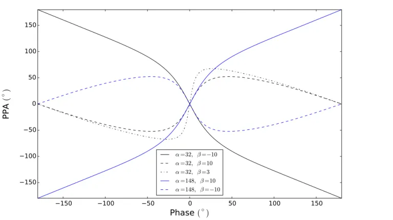
The RVM is a widely accepted beam model proposed by Radhakrishnan & Cooke (1969). This model was developed to explain the behavior of the PPA in the Vela pulsar. PPA is the angle between the projected direction of the magnetic axis and the plane of linearly polarized emission. Very often in radio pulsars this angle, as a function of pulse longitude, has an S-shape. Radhakrishnan & Cooke(1969) suggested that this behavior has a geometrical origin. In their model they assumed that the radiation originates in the neighbor of each magnetic pole. The emission beam is centred on the magnetic axis and occupies a region defined by the last open magnetic field lines. The beam shape is assumed to be conical. If we assume that the plane of linear polarization is tied on the magnetic field lines as the pulsar spins the projection direction rotates with the star and the PPA varies from 0 at the profile centre to, at most, 180◦. The RVM model calculates the PPA (Ψ) changes through pulse longitude using simple geometry and the Radhakrishnan & Cooke convention:
tan(Ψ0−Ψ) =
sinαsin(ϕ−ϕ0)
sin(α+β) cosα−cos(α+β) sinαcos(ϕ−ϕ0)
, (1.7)
whereϕis the rotational phase,αandβare the emission geometry angles,Ψ0andϕ0are the PPA and phase of the fiducial point, respectively.
The anglesαandβas well as other important geometry angles of this model are presented in Fig.1.4. The angleαdefines the inclination of the magnetic axis with respect to the rotation axis, and the impact parameter (β) represents the closest approach of the line of sight to the magnetic axis. Due to conventional reasons, the outer line of sightβis positive whenα <90◦
and negative whenα >90◦and for an inner line of sight andβis positive whenα >90◦and negative whenα <90◦6. In order for the pulsar to be visible in all casesβ ≤ρ, whereρis the
half-opening angle of the emission beam. We can detect emission for both magnetic poles (an interpulse) in cases whereα≳90◦−ρ.
According to the RVM model, the steepness and the curve shape of the PPA S-shape de-pends only on the emission beam geometry. The impact parameterβ controls how steep the shape will be. In the cases where the line of sight cuts the emission beam close to the centre, the PPA S-shape is steeper compared to the cases where the line of sight cuts the emission beam close to the edges. The inner or outer line of sight controls the curve shape. For the outer line of sights the PPA rolls over while for the inner line of sights it continues to rise. A few examples for inner and outer lines of sight are presented in Fig.1.5.
1.6. Modeling the radio emission beam
15
Figure 1.4: Geometry of the pulsar emission beam. The figure is based on Fig. 3.4
from
Lorimer & Kramer
(
2012
). For more details about the angles see the text.
Chapter
1.
Introduction
−150 −100 −50 0 50 100 150Phase (
◦)
−150 −100 −50 0 50 100 150PP
A
(
◦)
α =32, β =−10 α =32, β =10 α =32, β =3 α =148, β =10 α =148, β =−10Figure 1.5: The PPA as a function of pulse longitude. With filled lines we present outer line of sights, and with dotted lines inner
lines of sight. As mentioned in the text, the closer to the centre the line of sight cuts the emission beam the steeper the PPA is (see
the black dot-dashed line). For pulsars with pulse width
≲
30
◦there is often an 180
◦unambiguity in
α
since we cannot distinguish
between inner or outer line of sight (see black solid line (inner line of sight) and blue dotted line (outer line of sight)).
1.6. Modeling the radio emission beam
17
Each combination of the anglesαandβ gives a unique S-shape swing. By simple fitting of the RVM model to the observable PPA swing we can extract the geometry of the emission beam. However, very often RVM model solutions are not constrained. The reason is mostly because the emission longitude range of pulsars is small, only around 30◦. Having available only a small portion of the PA swing does not allow us to distinguish between an outer or inner line of sight, creating a 180◦ ambiguity onαmeasurements (see Fig.1.5). And partly because the PA swing is observed to deviate strongly from a simple S-shape. These deviations are caused either by propagation through the pulsar magnetosphere or thought the ISM.
With this very simple conical beam model, in which the magnetic axis is in the centre of the emission beam, we can also express the width of the pulse profile, using only the geomet-ric angles. While the pulsar is spinning, the trajectory of the line of sight follows a curved line through the emission beam. The length of this line is the profile width (w) and can be measured by applying simple geometry:
sin2 (w 4 ) =sin 2(ρ/2)−sin2(β/2) sinαsin(α+β) . (1.8)
It is worth noting that this equation is independent of the beam shape. While the anglesαand β depend only on the orientation of the emission beam, and can be measured through polar-ization observations, as described above, the opening angle is related to the shape, size and the location of the emission region. If we assume that the field lines are dipolar (a Goldreich-Julian-type beam,7Goldreich & Julian,1969), the radiation region is defined by the last open
field line, and the emission region is close to the polar cap, we can express the opening angle ρwith (Lorimer & Kramer,2012):
ρ≈1.24◦ √ rem 10 (km) 1 (s) P . (1.9)
It should be noted that this expression is only valid forρ≲30◦. In different cases the full last opening angle as expressed from Goldreich-Julian model should be applied. According to Eq.1.9, the knowledge of the opening angle requires an accurate measurement of the emission height (rem). The lack of a theoretical model, as mentioned above, requires emission heights to be determined observationally.
1.6.2
Radius-to-frequency mapping (RFM)
As mentioned earlier, the radio emission of pulsars is believed to originate in the open field lines in the magnetosphere. Even though the region of emission is known, the exact emis-sion height8 is still unknown but generally accepted to be within 10% to 30% of the
light-cylinder radius for canonical pulsars and MSPs, respectively (Kijak & Gil,1998). Observa-tionally (Rankin,1983;Gould & Lyne,1998;Johnston et al.,2008), we see that in general as the observing frequency increases profiles become narrower, outer components are more promi-nent, double peaks move closer together and the polarization fraction declines.
The model that is used to explain these observational facts is the RFM model (Cordes, 1978). The main idea is that high frequencies are emitted closer to the pulsar surface compared
7
General relativistic effects add, only, a 4% distortion on the Goldreich-Julian-type beam (Kapoor &
Shukre,1998).
8With emission heights we are referring to the heights in which the radiation leaves the magneto-