IT 13 061
Examensarbete 30 hp
September 2013
Benchmarking of Data Mining
Techniques as Applied to Power
System Analysis
Can ANIL
Institutionen för informationsteknologi
Department of Information Technology
Teknisk- naturvetenskaplig fakultet UTH-enheten Besöksadress: Ångströmlaboratoriet Lägerhyddsvägen 1 Hus 4, Plan 0 Postadress: Box 536 751 21 Uppsala Telefon: 018 – 471 30 03 Telefax: 018 – 471 30 00 Hemsida: http://www.teknat.uu.se/student
Abstract
Benchmarking of Data Mining Techniques as Applied
to Power System Analysis
Can ANIL
The field of electric power systems is currently facing explosive growth in the amount of data. Since extracting useful information from this enormous amount of data is highly complex, costly, and time consuming, data mining can play a key role. In particular, the standard data mining algorithms for the analysis of huge data volumes can be parallelized for faster processing. This thesis focuses on benchmarking of parallel processing platforms; it employs data parallelization using Apache Hadoop cluster (MapReduce paradigm) and shared-memory parallelization using multi-cores on a single machine. As a starting point, we conduct real-time experiments in order to evaluate the efficacy of these two parallel processing platforms in terms of
performance, resource usage (Memory), efficiency (including speed-up), accuracy, and scalability. The end result shows that the data mining methods can indeed be
implemented as efficient parallel processes, and can be used to obtain useful results from huge amount of data in a case study scenario. Overall, we establish that parallelization using Apache Hadoop cluster is a promising model for scalable performance compared with the alternative suitable parallelization using multi-cores on a single machine.
Tryckt av: Reprocentralen ITC IT 13 061
Examinator: Ivan Christoff Ämnesgranskare: Tore Risch Handledare: Moustafa Chenine
Page 1 / 75
Acknowledgements
This piece of work was conducted at KTH (Royal Institute of Technology) within the framework of the EU EP7 iTesla Project in Stockholm. First and foremost, I would like to give special thanks to my supervisor, Moustafa Chenine, for his patience, advice and constructive comments throughout the development of this thesis. I would also like to thank Miftah Karim for being a valuable source of ideas and guidance during the development of this thesis. I would like to express my gratitude to Tore Risch., my reviewer at Uppsala University, who reviewed my work and shared his worthwhile opinions; and also to Ivan Christoff, my examiner at Uppsala University, for his invaluable guidance leading to the completion of this work. Furthermore, my warmhearted thanks go to my adored family, and – last but not least – my warm thanks go to Melisa Bergström for her invaluable support.
Page 3 / 75
Contents
1. Introduction ... 8
1.1. Problem Statement ... 8
1.2. Aim and Objective ... 9
1.3. Delimitations ... 9
1.4. Thesis Structure... 10
2. Context of Study ... 11
2.1. The Electric Power System ... 11
2.2. Data Mining and Knowledge Discovery ... 11
2.3. Statistical Correlation ... 13 2.4. R (programming language) ... 13 2.5. Parallelization... 13 3. Related Works ... 21 4. Methodology of Study ... 23 4.1. Method ... 23 4.2. Functions ... 25 4.3. Case Study... 28
5. Implementation of the Study ... 31
5.1. Set-up and Configuration ... 31
5.2. Data Selection and Pre-processing ... 33
5.3. Implementation of the Standalone Modules ... 34
5.4. Implementation of the Case Study ... 44
6. Evaluation of the Study ... 46
6.1. Evaluation of the Standalone Modules ... 46
6.2. Case Study Evaluation ... 56
7. Conclusion and Future Work ... 64
References ... 66
Appendix ... 69
A. Standalone Modules ... 69
Page 5 / 75
List of Figures
Figure 1: The KDD Process, Step-by-Step ... 12
Figure 2: Map Reduce Example [2] ... 18
Figure 3: R and Hadoop Integration for Hadoop Streaming [2] ... 19
Figure 4: R and Hadoop Integration for RHadoop [2] ... 20
Figure 5: The Phases of Work ... 23
Figure 6: Development Work-Flow ... 24
Figure 7: Example of K-Nearest Neighbors Algorithms [22] ... 26
Figure 8: Example of K-means Clustering Algorithms [21] ... 27
Figure 9: Case Study Scenario Action Flow ... 30
Figure 10: The High-Level Architecture of Apache Hadoop Cluster ... 32
Figure 11: View of Processes After a fork() System Call ... 36
Figure 12: Flow Chart of Parallel Pearson's Linear Correlation Coefficient Algorithm Based on MapReduce ... 36
Figure 13: Flow Chart of Parallel kNN Algorithm Based on MapReduce ... 39
Figure 14: Flow Chart of Parallel K-means Algorithm Based on MapReduce ... 42
Figure 15: Performance for Stand-alone Modules…..…….... ... 47
Figure 16: Memory Usage for Stand-alone Modules……….. ... 49
Figure 17: Accuracy for Stand-alone Modules ... 50
Figure 18: Speed-up for Statistical Module on Platform-2 and -3 ... 51
Figure 19: Speed-up for Classification Module on Platform-2 and -3 ... 52
Figure 20: Speed-up for Clustering Module on Platform-2 and -3 ... 52
Figure 21: Efficiency for Statistical Module on Platform-2 and -3 ... 53
Figure 22: Efficiency for Classification Module on Platform-2 and -3 ... 54
Figure 23: Efficiency for Clustering Module on Platform-2 and -3 ... 55
Figure 24: Scale-up for Stand-alone Modules ... 55
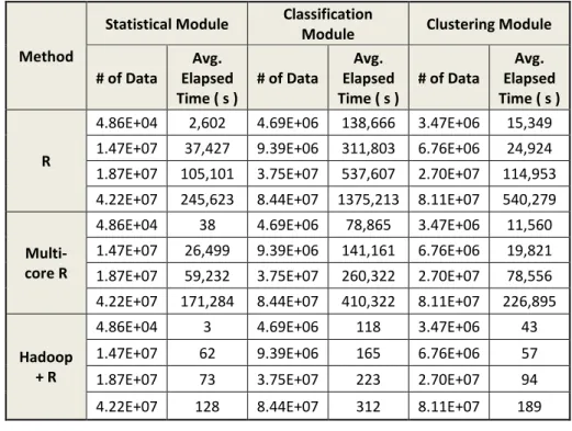
Figure 25: Comparison of Elapsed Time Spent by Different Platforms for the Data Mining Processes ... 57
Figure 26: Comparison of Memory Consumption by Different Platforms for the Data Mining Processes ... 59
Figure 27: Comparison of Accuracy by Different Platforms for Data Mining Processes ... 59
Figure 28: Speed-up for Data Mining Processes on Platform-2 and -3 ... 61
Figure 29: Efficiency for Data Mining Processes on Platform-2 and -3 ... 61
Figure 30: Scale-up for Data Mining Processes on Platform-2 and -3 ... 62
Figure 31: Prediction of Production Clusters by Cart Decision Tree ... 63
Figure 32: Pearson’s Linear Correlation Coefficient Matrix for Selected Nodes ... 70
Figure 33: Pearson’s Linear Correlation Coefficient Scatter Plot Matrix with Regression Analysis ... 71
Figure 34: kNN result for node A.OTHP3... 72
Figure 35: Pearson’s Linear Correlation Coefficient Values for threshold between - 0.3 and + 0.3 ... 74
Page 6 / 75
List of Tables
Table 1: Hardware and Software Information ... 32
Table 2: R Packages ... 34
Table 3: Average Elapsed Time Spends For Standalone Modules ... 47
Table 4: Memory Consumption for Standalone Modules ... 49
Table 5: Average Elapsed Time Spent for data mining processes ... 57
Table 6: Memory Consumption for Data Mining Processes ... 58
Page 8 / 75
Chapter 1
Introduction
In the last decade, the ongoing rapid growth of modern computational technology has created an astounding flow of data. As with other industries, the power system field is facing an explosive growth of data [5], and the development of the electric power industry has resulted in more and more real-time data being stored in databases. Besides the data from simulations, traditional remote field devices such as Remote Terminal Units (RTU); a great contribution to this explosive data is foreseen to originate from new measurement devices such as Phasor Measurement Units (PMUs) which would be utilized in Wide Area Monitoring and Control systems(WAMC) [5, 40]. Processing and interpreting this huge volume of data is extremely complex, costly and time consuming [6]. Data mining techniques [7, 40] may be used to extract useful information (i.e. knowledge) from the huge amounts of data; such as the correlation between power generation and consumption.
When properly trained up, pattern recognition algorithms in data mining can detect deviation from the regular data, which may be useful for triggering alarms and messages (classification) that provide important information to the operator. The mining and off-line analysis of historical data can provide knowledge that can be subsequently implemented online [8]. This knowledge might be related to fault analysis, energy consumption, analysis of distributed generation, or load pattern.
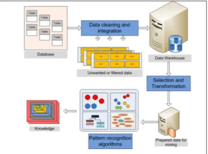
Knowledge Discovery in Databases (KDD) aims at extracting useful knowledge from data [9]. It is a process comprising several steps – selection of target data, data pre-processing, data transformation, data mining, and evaluation of patterns [9] – and it relies on databases management, machine learning and statistics. Knowledge discovery and machine learning based on pattern recognition can provide relevant knowledge to support power systems planning and operation.
1.1.
Problem Statement
The problem is that processing enormous amount of data using data mining techniques, while a good approach, could be time-consuming and slow [6]. One solution would be to apply parallel processing techniques to data mining, therefore this thesis focuses on:
How data mining algorithms can be parallelized.
Page 9 / 75
Testing those parallel data mining algorithms in a case study scenario (trialed in a case study scenario).
1.2.
Aim and Objective
The main aim and objective of this thesis is to implement data mining algorithms on parallel platforms and to evaluate them in terms of which parallel platform is the most efficient for performing data mining processes in the shortest amount of time. The gathered data are subjected to data mining processing on different parallel platforms with the aim of benchmarking (comparing) the parallel processing of data mining algorithms as applied to the power system data.
The workflow is as follows:
Devise data mining techniques and methods for implementing them on parallel platforms.
Implement the data mining functions for parallel platforms as standalone modules.
Reuse the standalone modules concurrently in the Case Study, to collect results.
Evaluate the outcomes.
1.3.
Delimitations
The scope of this thesis is the benchmarking of sequential and parallel implementations of data mining algorithms; this benchmarking being conducted on performance, resource usage (CPU and Memory), efficiency (including speed-up), accuracy and scalability.
Implementation of the decision-tree algorithm as a parallel process is excluded from the scope of thesis due to time limitations and the complexity of transforming the decision tree sequential algorithm to the MapReduce programming paradigm.
In this study, the size of the test beds that are used to conduct the analysis of parallel processes are limited by the use of one single machine with four cores (for parallel computing) and a small size of Apache Hadoop cluster size—four nodes (for distributed computing).
The study includes only one case study due to there being no feasible and implementable real use case scenarios for analyzing power systems.
Page 10 / 75
1.4.
Thesis Structure
Following this introductory chapter (chapter 1) the thesis continuous with chapter 2 which describes the general context of this study. In the subsequent chapters 3, 4, 5 and 6, I explain in details my approach to applying data mining techniques to power systems. Therefore, chapter 3 presents the related works, chapter 4 presents our methodology, chapter 5 introduces the reader to the implementation details of the work, and chapter 6 provides an evaluation details of the work. The final chapter presents conclusions and ideas for taking this work further are given in the final chapter.
Page 11 / 75
Chapter 2
2.
Context of Study
This chapter presents the background information that will help set the scene and give a better understanding of the subject matter for this study.
2.1.
The Electric Power System
Electric power systems are critical infrastructures for modern society [19, 34, and 35]. They span huge geographical areas, and comprise thousands of measurement and monitoring systems continuously collecting various data such as voltage and current, power lows, line temperatures, plus data relating to the stating of devices.
The increased utilization of information and communication technologies make available a wealth of data which can be used to gain a deeper understanding of the dynamics of the process as well as an opportunity to use data in online decision support.
For example, systems like Wide Area Monitoring and Control (WAMC) continuously collect data at a high sampling rate (e.g. 50 samples per second),where each sample can be several measurements [34, 35].
2.2.
Data Mining and Knowledge Discovery
Knowledge Discovery in Databases (KDD) is the process of discovering useful knowledge from a huge amount of data [5, 6, and 13]. This means preparing and selecting the data to be mined, cleaning the data, incorporating prior knowledge, and deriving solutions from the observed results.
While KDD is commonly used to refer to the overall process of discovering useful knowledge from data, data mining refers to the particular step in this process which involves the application of specific algorithms for extracting patterns from data. Data mining is defined as “the
nontrivial extraction of implicit, previously unknown, and potentially useful information from data” [16]. Thus the overall aim of the data mining process is to derive useful information / knowledge from raw data, by a process of transformation into a structure that is suitable for further processing or direct application [5, 6, and 13].
Page 12 / 75
Figure 1: The KDD Process, Step-by-Step
2.2.1 Data Mining Tasks
This section presents information about the various data mining methods.
2.2.1.1. Predictive:
This is a data mining task that uses certain variables to predict unknown or future values of other variables. It is achieved by subjecting a huge amount of data to a training regime known as supervised learning, whereby estimated values are compared with known results [13].
Classification: Given a set of predefined categorical classes, this task attempts to determine which of these classes a specific data item belongs to. Some commonly used algorithms in classification are C4.5, K-Nearest Neighbors (KNN) and Naï ve Bayes [9].
Regression: Uses existing values to forecast what other values will be. Simply, regression uses standard statistical techniques such as linear regression. But many real-world problems such as stock price changes and sales volumes do not lend themselves to prediction via regression, because they depend on complex interactions of multiple variables. Therefore, some other more complex techniques such as logistic regression or neural networks may be necessary in order to forecast future values. The same model types, such as Classification and Regression Trees (CART), can often be used for both regression and classification; its decision tree algorithm can be used to build both classification trees (to classify categorical response variables) and regression trees (to forecast continuous response variables). Neural nets can also be used to create both classification and regression models.
2.2.1.2. Descriptive:
No training data is used here, and it is sometimes referred to as unsupervised learning because there is no already-known result to guide the algorithms [9].
Clustering: Involves separating data points into groups according to how “similar” their attributes
Page 13 / 75
2.3.
Statistical Correlation
Correlation is a statistical technique that tells us whether two variables are related to each other— either positively or negatively, and to what degree (strength of correlation) [8].
One of the most common methods of computing correlation is Pearson’s linear correlation coefficient. Pearson's linear coefficient correlation (r) is a numerical value that ranges from + 1.0 to - 1.0, where r > 0 indicates a positive relationship and r < 0 indicates a negative relationship; and where r = 0 indicates there is no relationship between variables. The closer we get to +1.0 or -1.0, the stronger the relationship (positive or negative) between the variables [31].
2.4.
R (programming language)
R is a GNU project; it is an interpreted programming language which is typically used through a command line interpreter [33]. R is a highly efficient, extensible, elegant and comprehensive environment for statistical computing and graphics. The R programming language is used to develop parallel platforms. One of the important features of R is that it supports user-created R packages and a variety of file formats (including XML, binary files, .csv) [33].
2.4.1. Drawbacks of R
The most significant limitations of R are that it is single-threaded and memory-bound [20]:
It is single-threaded:
The R language has no explicit constructs for parallelization, such as threads. An out-of-the-box R installation cannot take advantage of multiple CPUs. Regardless of the number of cores on your CPU, R will only use one core by default.
It is memory-bound:
Whereas other programming languages read data from files as needed, R requires that your entire data set fits in memory (RAM) because all computation is carried out in the main memory of the computer. This is a problem because four gigabytes of memory (for example) will not hold eight gigabytes of data, no matter what.
2.5.
Parallelization
A large amount of computing resource (execution speed) and storage space (memory) is required to extract useful knowledge from large amounts of data [11]. Parallelization or distributed computing allows us to speed up computations by using multiple CPUs or CPU cores to run several computations concurrently. Although parallel and distributed computing are not exactly the same, they serve the same fundamental purpose of dividing large problems into smaller problems that can be solved concurrently.
Page 14 / 75
Execution Speed
Execution speed can be improved by parallelizing operations either a) within a processor using pipelining or multiple arithmetic logic units (ALUs), or b) between processors with each processor working on a different part of the problem in parallel [11].
Memory
The memory capacity of several machines can be utilized for parallel or distributed processing, to overcome the problem of no single machine having sufficient memory for processing of large data sets [11].
Concurrency
A single computing resource can do only one thing at a time whereas multiple computing resources can do many things simultaneously.
There are broadly two taxonomies of parallel or distributed computing, depending on the computation model (task / data parallelization) and communication model (message passing / shared memory) that is employed [11, 12]. Task parallelization splits computation tasks into distinct subtasks (different computation programs) that are assigned to different computing units, whereas data parallelization (master / slave architecture) involves all computing units running the same program but on different data. The message passing model involves messages being exchanged between different tasks (or computing units), whereas the shared memory model involves communication by reading / writing to a shared memory location.
This thesis focuses on the data parallelization using Apache Hadoop cluster (master-slave architecture and MapReduce paradigm), and shared-memory parallelization using multi-cores on a single machine.
2.5.1.
Parallel Computing with R
The R programming language is a sequential language. That is, program instructions are executed one-at-a-time in strict sequence from the top to the bottom of the program (subject control of flow operations such as loops and conditions). In contrast—parallel computing allows different program instructions to be executed simultaneously; or the same program instructions to be simultaneously on different data.
In recent years, a great number of studies [39] have focused on the problem of extensive analysis, some researchers in the open source R community have developed high computing packages that provide R scripts able to run on clusters or multi-core platforms. According to [39], there are two general schemes of parallel computing R packages; “building blocks” and “task
farm”. The first scheme offers basic parallel building blocks such that a parallel implementation of an algorithm can be developed, whereas latter is where a 'master' process (node) feeds a pool of 'slave' processes (nodes) with subtasks. Typical uses are performing the same algorithm on each slave node with different data; or perform different analysis on the same data. Thus, there are several ways to parallelize the sequential R language with high-performance computing R packages
Page 15 / 75
[20, 39]. One other option could be to start an R session on each of several computers, and effectively run the same program on each of them. Other possibility could be to use Apache Hadoop framework as distributed computing [20].
In the following we describe in detail master-slave architecture (which is analogous to “task
farm” parallelization of taxonomy) and shared-memory parallelization (which is analogous to
“building blocks” parallelization of taxonomy).
2.5.1.1. Shared Memory Parallelization (Parallel Computing)
In this parallelization, tasks share a same address space to read and write (asynchronously) [14]. Multi-core architecture is defined to a single processor packages that has two or more processor execution cores [24]. In a multi-core microprocessor, each core solely performs optimizations such as pipelining and multithreading. Further, in a multi-core microprocessor, with divide-and-conquer strategy multi-core architecture carries out more work in a given clock cycle [24].
Since all threads run on the same computer there is no need for network communication in a multi-core parallelization. On the other hand, as every thread has access to all objects on the heap there is a extensive need for concurrency control to not to violate data integrity as parallelization of the program[11]. A great way to provide concurrency is using locks [11]. Compared to master-slave parallelization, constructing shared-memory parallelization reduces the overhead of communicating through a network. Shared memory parallelization with R is currently limited to a small amount of parallelized functions [39]. A key advantage of shared-memory parallelization is data sharing among the tasks are fast and uniform [14]. On the other hand, the main drawback is the lack of scalability between memory and CPUs. Adding more CPUs could dramatically increase traffic on the path between shared-memory and CPU [14].
2.5.1.1.1. Multi-core R Package
Multi-core is a popular parallel programming package that was written by Simon Urbanek in 2009 for use on multiprocessor and multi-core computers on a single machine [32]. It does not support multiple cluster nodes. It immediately became popular due to its smart use of the fork() system call which allows us to implement a parallel lapply() operation that is even easier to use than the Simple Network of Workstations (SNOW) parLapply( ) [36]. Unfortunately, since fork() is a Posix system call, multi-core can’t really be used on Windows machines. Nevertheless, multi-core works perfectly for most R functions on Posix systems such as Linux, and its use of fork() makes it very fast and suitable. It is distinguished from other parallelization solutions because multi-core jobs all share the same state when they are spawned. Compared to the SNOW package on a single machine, the multi-core package is more efficient than SNOW because fork() only copies data when it is modified [20].
Page 16 / 75 Advantages [32]:
Able to load-balance with multi-core.
Able to set the number of cores.
Fast.
Overcomes the single-threaded nature of R.
Easy to install and use.
Disadvantages [32]:
Does not work in Microsoft Windows.
Need high memory hardware.
2.5.1.2. Master-slave Parallelization (Distributed Computing)
In this parallelization , a large data set is usually split into smaller pieces and distributed through the cluster by the main computation node—the master node, a subtask for its subsets are solved by other computing nodes—the slave nodes. The slave nodes do not communicate each other, they responsible to execute the task and return the result to master, while the master node is responsible to start the slave nodes. This type parallelization is very suitable for clusters or supercomputers and MapReduce paradigm [2, 3, and 40]. Since each slave node has own local memory space, this type of architecture can be defined as distributed shared memory as well [14]. While the load-balancing of the computing nodes is well handled, the parallelization scales linearly with the number of computing nodes [11]. Another advantage for this parallelization is each computing node can easily access its own memory without any interference and the overhead [14].
2.5.1.2.1. Apache Hadoop Project
Apache Hadoop is a first class open-source project hosted by Apache Software Foundation [2, 3]. It is a framework that makes it possible to process huge data sets through clusters of computers using basic programming models. Apache Hadoop does not rely on hardware in order to provide high-availability; the software library is designed so that it can detect and handle failures at the application layer [2, 4]. The storage and computational capabilities are designed so that it scales up from a single server to thousands of machines [2], with each machine providing its own storage and computation.
The Apache Hadoop framework comprises eleven sub-projects that provide distributed computing and computational capabilities. Although Hadoop MapReduce and Hadoop Distributed File Systems (HDFS) are known and used widely [3], other projects provide supplementary functions.
Page 17 / 75
Hadoop is a distributed master-slave architecture which has two main components: HDFS for storage and MapReduce for computational capabilities. One of the biggest benefits of the Hadoop ecosystem is that it can be integrated with any programming language, such as R or Python [2, 3].
A-Hadoop Distributed File Systems (HDFS)
Apache Hadoop comes with a distributed file system called HDFS, which stands for Hadoop Distributed File System. It is ideal for storing large amounts of data (terabytes and petabytes) [2]. HDFS provides seamless access to files that are distributed across nodes in different clusters, and those virtual files can be accessed by the MapReduce programming model in a streaming fashion. HDFS is fault-tolerant and it provides high-throughput access to large data sets [1, 2].
HDFS is similar to other distributed file systems, except for the write-once-read-many concurrency model [1] that simplifies data coherency and enables high-throughput access. Some of the notable HDFS features are [1, 2]:
Detection and quick automatic recovery from faults.
Data access via MapReduce streaming.
Simple and robust coherency model.
Enable portability between very different commodity operating systems and hardware.
Scalability to store and process large amounts of data.
Distribution of data and logic to nodes where data is located, for efficient parallel processing.
Reliability, resulting from maintaining multiple copies of data and automatically redeploying processing logic in the event of failures
B-Hadoop Map-Reduce
MapReduce was popularized in a Google paper, “MapReduce: Simplified Data Processing on
Large Clusters” [1] by Jeffrey Dean and Sanjay Ghemawat. In the time since Google built their own implementation to churn web content, MapReduce has been applied to other problems [1].
MapReduce is a data parallelization programming model—the dataset is split into independent subsets and distributed, then the same instructions are applied to each subset in concurrently [42] , for processing and generating huge amounts of datasets [2, 3]. It is inspired by functional languages and is aimed at data-intensive computations, such as Google’s original use to regenerate the index of the World Wide Web [31].
The MapReduce model outlines a way to perform work across a cluster of inexpensive commodity machines. Simply put, there are two phases: Map and Reduce. Although the input to MapReduce can vary according to application, the output from MapReduce is always a set of (key, value) pairs. The programmer writes two functions, the Map function and the Reduce function as follows:
The Map function is applied to the input data, and produces a list of intermediate (key, value) pairs that can vary according to application, algorithm, and programmer.
Page 18 / 75
The Reduce function is then applied to the list of intermediate values (map function outputs) that have the same key. Typically this is some kind of convergence or merging operation which produces (key, value) pairs as output.
A key benefit of the MapReduce programming model is that the programmer does not need to deal with the complicated code parallelization, and can therefore focus on the required computation A simplified version of a MapReduce job proceeds as follows:
Map Phase
1. Each cluster node takes a piece of the initial huge amount of data and runs a Map task on each record (item) of input. You supply the code for the Map task.
2. All of the Map tasks run in parallel, creating a key/value pair for each record. The key identifies the item’s fragment for the Reduce operation. The value can be the record itself or some derivation of it.
The Shuffle (Hadoop does this phase automatically)
1. At the end of the Map phase, the machines all pool their results. Every key/value pair is assigned to a fragment, based on the key. (Hadoop does this automatically)
Reduce Phase
1. The cluster machines then switch roles and run the Reduce task on each pile. You supply the code for the Reduce task, which gets the entire pile – that is, all of the key/value pairs for a given key – at once.
2. The Reduce task typically (but not necessarily) emits some output for each pile.
Figure 2provides a visual representation of a MapReduce flow as an example. Let's consider an input in which each line is a record of the format (letter and number), and the aim is to find the maximum value of number for each letter. Step (1) describes the raw input. In Step (2), the MapReduce system provides each record’s line number and content to the Map process, which splits the record into a key (letter) and value (number). The Shuffle step gathers all of the values for each letter into a common bucket, and feeds each bucket to the Reduce step. In turn, the Reduce step plucks out the maximum value from the bucket. The output is a set of (letter, maximum number) pairs.
Page 19 / 75
2.5.1.2.2. Integration with R and Apache Hadoop Project
A. R and Apache Hadoop Streaming
With Hadoop Streaming, the Map and Reduce functions can be written in any programming language or script that allows the reading of data from standard input and the writing of data to standard output. R supports this feature, so it can easily be used with Apache Hadoop framework; as illustrated in Figure 3, R and Hadoop Streaming can be used to process data in a MapReduce job just like the regular MapReduce.
Using Apache Hadoop framework overcomes the single-threaded and memory boundary limitations of R. Another big advantage is that Hadoop provides scalability. The only drawback is that the implementation breaks up a single logical process into multiple scripts and steps due to MapReduce programming framework.
Figure 3: R and Hadoop Integration for Hadoop Streaming [2]
B. RHADOOP
There is another way to integrate R and Apache Hadoop framework—using the RHadoop open source project created by Revolution Analytics. RHadoop allows users to use MapReduce interactions directly from within R without touching Hadoop so much.
RHadoop consists of two components:
Rmr: This R package allows an R programmer to perform statistical analysis via MapReduce on a Hadoop cluster. The rmr package uses Hadoop streaming, and one of the most important features of rmr is that it makes the R client-side environment available to the Map and Reduce functions of R that are executed in MapReduce. The integration between R and Hadoop via RHadoop as depicted in Figure 4.
Page 20 / 75
Figure 4: R and Hadoop Integration for RHadoop [2]
Rhdfs: This R package provides basic connectivity to the Hadoop Distributed File System (HDFS), enabling programmers to browse, read, write, and modify HDFS files.
Page 21 / 75
Chapter 3
3.
Related Works
In recent years, a great number of studies [37] have investigated parallel data mining methods, with a view to making them faster via different implementations. Most research on parallel data mining [38] has focused on the efficient parallelization of distributed computing, but – because almost every computer has multiple cores nowadays [11] – shared memory parallelization (implicit parallelization) has become popular. Parallel data mining algorithms are proposed for symmetric multiprocessing (SMP) in [40, 42]. McKmeans [11] discusses thread programming, whereby a sequential program is split into several tasks which are then processed as threads. The paper introduces highly efficient multi-core parallelization of k-means; parallelized by simultaneously calculating by the minimum distance partition and the centroid update. The results are compared to sequential K-means R and McKmeans parallel implementation (similar way of parallel implementation of k-means clustering in implicitly) in terms of runtime performance for various datasets. In the other paper [42], the split data points are handled in agents rather than threads. Different parallel k-means algorithms are compared based on runtime performance, these algorithms being: paraKmeans [41], sequential R and clojure [42]. Performance characterization of individual data mining algorithms has been documented in [43], a paper which focuses on the CPU performance and cache (memory) behaviors of data mining applications such as association rule mining, clustering, and classification. Ying [44] presented MineBench as a benchmarking suite which comprises data mining application, plus evaluation of classification, clustering and ARM categories of data mining applications with implemented using C/C++. They show that the performance is impacted by synchronization overheads and I/O Time rather than by OS overheads and the overall performance of the data mining applications. Most of the parallel data mining algorithms for classification and clustering based on MapReduce [23, 25, and 27] are implemented in similar way to our implementations in this thesis, although the different tools are used—such as Weka [45].
Since R is a very widely used statistical tool, many studies have been done to adapt it for parallelization platforms; thus many R parallel packages have been developed—such as RMPI, SNOW, and SPRINT [36]. Another work in this area is introduced and evaluated in [39]: parallelization for Pearson correlation. This introduced the simple parallel R interface (SPRINT) framework for HPC (High Performance Computing) systems. This study is very similar to our study in terms of the parallelization method, since we have used another common parallel (High Performance Computing) R package; the multi-core R package. Many of the other R parallel packages could be investigated in depth as a future study.
Page 22 / 75
Most of the previous work either focuses on specific data mining methods such as classification, clustering and association rules, or is limited to one particular programming language such as Java, or C. Examples include: Yanyan et al [23], Vineeth et al [43], and Ying et al [44]. Most of these compare the performance of data mining methods only in terms of runtime and speed up [23, 25], whereas in our thesis, we provide a comprehensive study of parallel data mining algorithms benchmarked with five different metrics. In addition to runtime and speedup, we also investigate scalability, efficiency, resource usage (Memory) and accuracy metrics.
To our knowledge there exists no evaluation of data mining algorithms based on our performance metrics—scalability, efficiency, and resource usage (Memory)—when implemented using the R programming language either with distributed Hadoop MapReduce framework or multi-core R parallel package prior to this work.
Page 23 / 75
Chapter 4
4.
Methodology of Study
This chapter presents the phases of work, the functions, and the case study.
4.1.
Method
Figure 5 shows the steps that were followed to achieve the desired goals, with these steps being described in detail in the sections that follow.
Figure 5: The Phases of Work
4.1.1. Literature Review
The literature review was carried out first to understand the parallel programming models and data mining techniques, and most of the material has been included in chapter 2 as background material. Since the programming language chosen for the project was R, additional investigation was needed to discover how tasks could be parallelized in R. The resources for the literature review were collected from Internet sources including published technical papers.
4.1.2. Design
The design phase of the project began with the selection of data mining algorithms appropriate to electric power system analysis [13] and to the aims of the thesis; it continued with the selection of parallelization models. It was decided to use two different parallel models: parallel programming using multi-cores via R packages, and MapReduce with the Apache Hadoop framework. The memory-bounded and single-threaded limitations of the R architecture were considered. The Apache Hadoop framework was selected as the most suitable solution for our kind of data: huge and stored (like log files—not updated frequently). Other factors in choosing the Apache Hadoop framework were that it is compatible with all languages, it has distributed file system, provides fault tolerance [2,24], and imposes no limitations on the data format or size. Hadoop and R could be integrated with RHadoop [20] and Hadoop Streaming [20], and the R multi-core package was used
Page 24 / 75
in order to facilitate multi-core computing.
4.1.3. Implementation
Since the main aim of the project was to extract useful knowledge from the huge data, prior to the development phase we created a case study (shown later in Figure 9). Therefore we could divide the development phase into two sections: standalone modules and case studies. The first statistical module was implemented in a sequential way, then implemented in a multi-core way, and finally implemented for Hadoop. Other modules were implemented in similar fashion as shown in Figure 6, and these modules were run concurrently for the case study.
Figure 6: Development Work-Flow
4.1.4. Selection of Metrics
The selection of metrics for this work included:
Performance:
The elapsed execution times of programs were measured, to find out which functions ran fastest on various platforms.
Memory Consumption:
The memory consumption (in megabytes) was measured, to determine the memory consumption of the platforms while running functions in practice.
Accuracy:
The purpose of accuracy comparison was to find out the correctness of the platforms' results when running the parallel (with Hadoop and with multi-core) and sequential models.
Page 25 / 75
Efficiency:
Efficiency tells us how much of the available processing power is being utilized, which we can measure using the formula:
Efficiency = Speedup / p, where p is the number of cores or nodes [26, 28]. Thus we are calculating Efficiency as the speedup per processor (core or node).
The Speedup itself is measure of how the execution time is improved by parallelization; it can be expressed as the ratio of the sequential execution time to the parallel execution time as follows:
Speedup (n) = T (1) / T (n), where n is the number of computing nodes. T(1) is the execution time of the tasks in series on 1 computing node or core, and T(n) is the execution time of the tasks in parallel with n computing nodes or cores [26, 28].
Scale Up ( scale vertically):
Scale Up is a measure of how the system and data size can grow as a result of parallelization. It can be expressed as follows:
Scale up (n) = T (1, D) / T (n, nD) where n is the number of computing nodes or cores, T (1, D) is the execution time of the tasks on 1 computing node or core with data size of D, and T (n, nD) is the execution time of the parallel tasks on n computing nodes or cores with data size of n times D [29].
Simply put, Scale up is defined as the ability of a larger system (n-times larger) to perform a larger job (n-times larger) in the same time as the original system.
4.1.5. Evaluation
After the metrics were selected, the evaluation was done in two ways: evaluation of the standalone modules, and then evaluation of the case study (with the standalone modules used concurrently).
4.1.6. Result
In order to achieve the aims of this thesis, the standalone modules were evaluated in terms of their suitability for parallel data mining, and the case study was brought to a conclusion with a CART decision tree.
4.2.
Functions
This section represents the functions for this work, including:
Pearson's Linear Correlation Coefficient
In order to calculate correlations between node pairs, Pearson’s linear correlation coefficient (r) function was used. The function is as follows [31]:
Page 26 / 75
Equation 1: Equation for Pearson’s linear correlation coefficient
K-Nearest Neighbor Classification ( kNN )
KNN is a supervised instance-based learning algorithm used for classifying objects based on closest training examples in the feature space. The kNN algorithm is relatively simple: it classifies an object according to the majority vote of its neighbors, so that the object is assigned to the class most common amongst its K nearest neighbors. There is no one-size-fits-all optimal number for the choice of K, and a good choice is often derived through heuristic approaches such as cross-validation. Choosing a large value for K could reduce the effect of noise, but it could result in computation inefficiency and the “blurring” of class boundaries. Hence a small positive integer is typically chosen for practical implementation, and in a special case where K = 1 (the nearest neighbor algorithm) the object is simply assigned to the class of its nearest neighbor. The selection of K-nearest neighbors is based on the distance between two data points in the feature space, with Euclidean distance usually being used as the distance metric. For every unknown instance, the distance between the unknown instance and all the instances found in the training set is calculated. The K instances in the training set that have the nearest distance to the unknown instance are selected, and the unknown instance will be assigned the class of the dominating neighbors. Figure 7 illustrates the kNN algorithm for a two-class example.
Figure 7: Example of K-Nearest Neighbors Algorithms [22]
The unknown instance (denoted as green circle) should be classified either as a blue square or a red triangle. If k = 3 (denoted by the inner circle), it is classified as a red triangle because there are two squares and only one square. If k = 5 (denoted by the outer circle), it is classified as a blue square because there are now three squares vs. two squares.
Algorithm
A high level summary of the nearest-neighbor algorithm method is shown below. The algorithm computes the distance (or similarity) between each test example z = (x', y') and all the training examples (x, y) E D to determine its nearest-neighbor list, Dz. Such computation can be costly if the number of training examples is large. However, efficient indexing techniques are available to reduce the number of computations needed to find the nearest neighbors of a test example.
Page 27 / 75
1: Let n be the number of nearest neighbors and D be the set of training examples 2: for each test example z0 (x’, y’) do
3: Compute d (x’, x), is the distance between z and every example of D. 4: Set of k closest training examples to z
5: y’= argmaxv
∑
(xi, yi)∈ Dz I (v= yi) 6: end for K-means Clustering
K-means is a method of cluster analysis whereby a set of data points (n) is partitioned into a number of clusters (k) such that each data point belongs to the cluster with the nearest mean. It is one of the simplest clustering algorithms, and its aim is to calculate sum-of-squares distances within the clusters.
Given a set of data points (x1 , x2 , ..., xn ) where each point is a d-dimensional vector, following the assignment to k centroids (μ1 , μ2 , ..., μk ) we will have k partitions S = {S1 , S2 , ..., Sk }.
The K-means function can be written as follows:
Equation 2: Equation for K-means Clustering Function
Figure 8: Example of K-means Clustering Algorithms [21]
Step 1: In the Figure 8 (a), K initial “means” are arbitrary selected within the data set. In this example the cluster number k = 3 so that the first clusters are red, green and blue ones.
Page 28 / 75
nearest mean.
Step 3: In the Figure 8 (c), the centroid of each of the k clusters is centered on new mean. Since K-means is an iterative algorithm, Step 2 and Step 3 are repeated until there is no convergence. In the Figure 8 (d) is the final result of clusters and its centroids.
Classification and Regression Trees
Classification and Regression Trees (CART) is a nonparametric binary recursive partitioning procedure that is introduced as an umbrella term for the following types of decision trees:
Classification Trees in which the target variable is categorical. The classification tree is used to identify the class within which a target variable would likely fall.
Regression Trees in which the target variable is continuous and the regression tree is used to predict its value. Trees are grown to maximum size without any stopping rule, and then branches are pruned back split-by-split to the root. The next split to be pruned is the one that is contributing least to the overall performance of the tree on training data [13].
The CART algorithm comprises as a series of questions, each of which determines what the next question (if any) will be. The result is a tree structure whose branches end with terminal nodes that represent the points at which no more questions will be asked (and the deduced solutions can be found).
4.3.
Case Study
Innovative Tools for Electrical System Security within Large Areas (iTesla) is a collaborative R&D project co-founded by the European Commission with a primarily goal of developing and validating an open interoperable toolbox for the future operation of the Pan-European grid. The iTesla project requires a great deal of data mining investigation in order to:
Manage statistical post-treatments of power system simulations.
Chain up data mining modules required for security analysis, and insert data mining features within the power system work flow.
Feed power system studies and processes with data.
In order to fulfill the data mining demands of the iTesla project, one real-life case scenario (case study) is used in this thesis.
Page 29 / 75
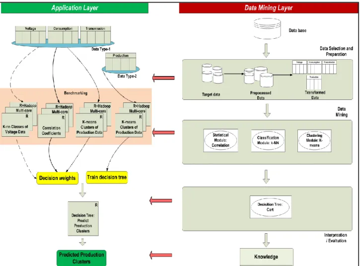
Case Study Scenario :
The purpose of carrying out this case study scenario is to predict future production results (clusters) for the benefit of power system control and operations. In order to provide (predict) these clusters, four different types of real-time power system data are used: voltage, consumption, transmission and production.
The main reason for the classification of voltage data – into high voltage, low voltage, normal voltage and abnormal voltage – is to understand different patterns in the data set based on the voltage magnitudes. This kind of classification is highly significant in understanding power system events and their associations to the voltage magnitudes. Later in the data mining process, the result classes of the classification module will be used to derive decision weights when developing the decision tree.
The main reason for finding correlation coefficient values between consumption data and voltage magnitudes is that – since strong correlation exists between power system events and voltage magnitudes – other parameters might also refer to valid patterns that are highly correlated to voltage magnitudes. Highly correlated consumption and transmission data will be subjected to further analysis, with the highly correlated consumption data being used to derive decision weights when developing the decision tree.
The main reason for finding k-means clusters on the consumption data is that it is a very useful pattern because generation and transmissions are highly correlated to the consumption data. Thus, each consumption cluster refers to a respective transmission and generation scheme. There will be five consumption clusters: very low, low, medium, high and very high clusters. Later of the data mining process, the result classes of the classification module will used to derive decision weights when developing the decision tree.
The main reason for finding k-means clusters on the production data is to use these clusters as training data, while developing the decision tree. The cluster number of (k=5) is used for clustering production data. Previous standalone modules are used and compared based on different platforms, thus classification (kNN), clustering (K-means) and statistical correlation (Pearson’s linear) functions are applied to these data sets. After the required data mining processes are applied, a final data mining process (CART decision tree) is applied based on previous results; the predictions of production clusters are found, and the results (predicted pattern) are plotted as a CART tree.
Page 30 / 75
Page 31 / 75
Chapter 5
5.
Implementation of the Study
This implementation chapter comprises four main parts. The first is the setup and configuration of the programming language, its packages, and Apache Hadoop cluster. The second part is about the data and its preparation. The third part is about implementation of the algorithms for three chosen modules and the decision tree function. The fourth and final part is the subsequent running of the modules concurrently in the context of the use case scenario (case study).
5.1.
Set-up and Configuration
The experiment is carried out on three different platforms as follows, with the implementation language being R and the operating system being Ubuntu Linux in all cases.
For Platform-1 a single machine (machine-1) is used, and only the R language is installed (for sequential processing).
For Platform-2 a single machine (machine-1) is used, and parallelization is achieved by combining R with the multi-core package.
For Platform-3, the four machines detailed in
Table 1 is used. These machines are arranged as a Hadoop cluster with machine-1 as a master and the other machines as slave nodes.
Information’s / Machines Machine - 1 (Master) Machine – 2 (Slave-1) Machine – 3 (Slave -2) Machine – 4 (Slave -3)
Processor Intel® Core™ i5-2410M CPU @ 2.30GHz × 4
Intel® Core™ 2 Duo CPU E6750 @ 2.66 GHz × 2
Intel® Core™ 2 Duo CPU E4600 @ 2.40 GHz × 2
Intel® Core™ 2 Duo CPU E4600 @ 2.40 GHz × 2 Memory 3.8 GİB DDR2 1.9 GİB DDR2 1.9 GİB DDR2 1.9 GİB DDR2 Os Type 64-bit 64-bit 64-bit 64-bit
Operating System
Ubuntu 12.10 Ubuntu 12.10 Ubuntu 12.10 Ubuntu 12.10
Page 32 / 75
Apache Hadoop Version
1.0.4 1.0.4 1.0.4 1.0.4
Table 1: Hardware and Software Information
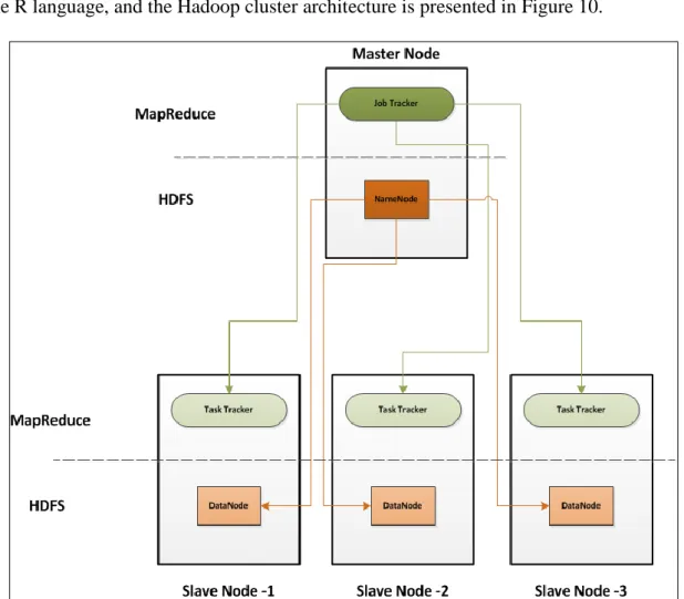
Since Platform-3 will be used for parallel R based on MapReduce, the Apache Hadoop installation and configuration is done on all four machines. RHadoop is installed on all computing nodes along with the R language, and the Hadoop cluster architecture is presented in Figure 10.
Page 33 / 75 Configuration of Hadoop Clusters:
As depicted in Figure 10, there is one master node and three slave nodes. The following configurations are necessary in order to set up one machine as the master and the other machines as slaves. One machine (master) in the cluster is designated as the NameNode and Jobtracker. The other machines in the cluster act as a “worker nodes” which are simply slave nodes that act as Data Node and TaskTracker (Figure 10)
5.2.
Data Selection and Pre-processing
The implementation begins with the selection of data from the huge database. The datasets were selected based on the requirements of the case study scenario; therefore four different data sets were selected:
Voltage Data: The voltage data represents the voltage values between two points, which in
our case are nodes. In power systems, the voltage ranges from low-voltage to ultra-high voltage [10].
Consumption Data: The consumption data represents the voltage values for the electrical energy that is used by all the various loads on the power system. In addition, consumption also includes the energy used to transport and deliver the energy [10].
Transmission Data: The transmission data represents voltage values which are used by the
power system to transport electrical energy efficiently over long distances to the consumption locations [10].
Production Data: The production data simply represents voltage values that are produced by the power system [10].
Since the data is gathered in real time and this project is carried out under the umbrella of the iTesla project, the data sets were handed over to us as a raw data in the .csv file. In order to make these data sets suitable for data mining purposes, they were subjected to operations such as data cleaning (including removal of out-of-range values), data merging, and transformation into the required file format. All of the data selection and pre-processing operations were done sequentially using by the R language. Listing 1 illustrates an example of the code (for data cleaning) is as follows:
Page 34 / 75
Listing 1: Source Code for Data Cleaning
5.3.
Implementation of the Standalone Modules
This section details the implementation of the algorithms for the three different modules. To begin, Table 2 lists all of the R packages that are used for the implementation phase.
Title Version Description
multicore 0.1-7 Parallel processing of R code on machines with multiple cores or CPUs.
class 7.3-7 Provides various functions for classification.
rmr2 2.2.0 Allows statistical analysis to be performed via MapReduce on a Hadoop cluster using the R programming language.
rhdfs 1.05 Provides basic connectivity to the Hadoop Distributed File System (HDFS) so that R programs can read, write, and modify files.
outliers 0.14 Provided to test for outliers.
corrgram 1.4 Allows us to plot a diagram.
lattice 0.20-15 A powerful and elegant high-level data visualization system.
rbenchmark 1.00 Benchmarking routine for R.
stats 2.15.3 This package contains functions for statistical calculations and random number generation
utils 1.23.2 Provides various programming utilities.
rpart 4.1-1 A toolkit for regression trees and recursive partitioning.
partykit 0.1-5 A toolkit that allows tree structure regression and classification models to be represented, summarized and visualized.
Table 2: R Packages
5.3.1. Statistical Module
This section presents the three implementations of the Pearson's linear correlation coefficient: sequential, parallel based on multi-core, and parallel based on MapReduce.
data.df<-read.table("Production.csv",sep=',',header=T) # Read the csv file with header data_orig<-data.df[-c(1:3),] # Data cleaning Begin colnames(data_orig)<-NULL data_orig<-t(data_orig) colnames(data_orig)<-data_orig[1,] data_orig<-data_orig[-1,] diff<-which(apply(data_orig,2,FUN = function(x){all(as.numeric(paste(x)) == 0)})) dat<-data_orig[,diff]
Page 35 / 75
5.3.1.1. Sequential:
In order to implement Pearson’s linear correlation coefficient in a sequential way (in Listing 2), the simple R language cor() function is used like this:
Listing 2: Source Code of Pearson’s Linear Correlation Coefficient in a Sequential Way
5.3.1.2. Parallel based on Multi-core:
In order to implement Pearson’s linear correlation coefficient in a parallel way using all possible cores on one computer (machine), the high-performance computing R multi-core package is used.
For this type parallelization we do not implement or transform the sequential Pearson's Correlation functions, we just increase the computing power. First we divide the computation into as many jobs as there are cores, with each job possibly covering more than one value (load balancing).
We use high level functions of multi-core mclapply() package – a parallel version of lapply() – to carry out the parallelization. Workers are started by mclapply() using the fork() function that provides an interface to the fork system call. Also, a pipe is set up that allows the child process to send data to the master, and the child’s standard input (stdin) is re-mapped to another pipe held by the master process.
The fork system call ( in Figure 11) spawns a parallel child copy of the parent (master) process, such that – at the point of forking – both processes share exactly the same state including the workspace, global options, and loaded packages. Fork is an ideal tool for parallel processing because data, code, variables and the environment of the master process are shared automatically from the start; there is no need to set up a parallel working environment, and explicit worker initialization is unnecessary.
Although mclapply() creates worker processes every time it is called, it is relatively fast because of copy-on-write; and the worker data is in synchronized with the master every time – forking the workers every time mclapply() is called gives each of them a virtual copy of the master’s environment right at the point that mclapply() is executed – such that the master’s data environment doesn’t need to be recreated in the workers. This function also gives you power of control over the number of cores that you want to use, via the mc.cores argument.
Page 36 / 75
Figure 11: View of Processes After a fork() System Call
Listing 3 shows the usage of the mclapply() function for Pearson’s linear correlation coefficient on the voltage data set is as follows:
Listing 3: Source Code of Parallel Pearson’s Linear Correlation Coefficient based on Multi-core
5.3.1.3. Parallel based on MapReduce:
In order to run the statistical module on the Hadoop cluster, the sequential Pearson’s linear correlation coefficient function has to be transformed into a MapReduce programming model. Figure 12 shows the MapReduce flow for Pearson’s linear correlation coefficient function. Since we
use only Hadoop Streaming, we create two R scripts: one for map and other for reduce.
Figure 12: Flow Chart of Parallel Pearson's Linear Correlation Coefficient Algorithm Based on MapReduce
possibleCores <- as.numeric ( system (" sysctl hw.ncpu | awk '{ print $2 }' ", intern=TRUE ) ) corr <- mclapply( mc.preschedule=TRUE, pair, mc.cores = possibleCores, colCor, mc.cleanup = TRUE )
Page 37 / 75
The algorithm of the MapReduce Pearson’s linear correlation coefficient function is as follows:
Map Function:
In the map function, we read the data from the HDFS line-by-line. Since we know that the MapReduce paradigm works only with <key, value> pairs, we create two lists to hold values and keys (valuePairs and keyPairs) respectively. Then we send the keys and values in the cat append as shown in Listing 4.
Listing 4: Source code of Map Function for Parallel Pearson’s Linear Correlation Coefficient Based on MapReduce
The Sort Phase:
After emitting the <key, value> pairs, and before these pairs are used by Reduce function, they will be sorted based on their key values. This sort operation is done by the Apache Hadoop framework automatically.
Reduce Function:
In the reduce function as shown in Listing 5, the incoming ordered <key, value> pairs are separated. The values which have the same key are simply combined in a list, and sent to the correlation function that computes the Pearson’s linear correlation coefficient. Our Reducer emits <K3, V3> where K3 is the pair of i-th and j-th column indices (they are unique) and V3 is the Pearson’s linear correlation coefficient. In the Figure 12 <K3, V3> is corresponding to < AB, r >.
Listing 5: Source code of Reduce Function for Pearson’s Linear Correlation Coefficient valuePair <- combn(fields, 2,simplify = F) #value pairs
uniqueKeyNumber=((length(fields))*((length(fields)-1))) / 2
keyPair=unlist(keyPairVector<-(1:uniqueKeyNumber)) #key pairs
cat(keyPair[[i]],valuePair[[i]],"\n",sep="\t") #output of map function
if( identical(preKey, "") || identical(preKey, key)) { preKey <- key
value1.vector <- c(value1.vector,value1) value2.vector <- c(value2.vector,value2)
} else { calculateCorrelation(preKey, value1.vector,value2.vector) preKey <- key
value1.vector <- numeric(0) value2.vector <- numeric(0)
value1.vector <- c(value1.vector,value1) value2.vector <- c(value2.vector,value2) }}
Page 38 / 75
5.3.2. Classification Module
This section presents the implementation of the kNN function in a three different ways: sequential, parallel based on multi-core, and parallel based on MapReduce.
5.3.2.1. Sequential:
In order to implement the kNN function in a sequential way, we simply use the knn() function from the R class package in Listing 6 as follows:
Listing 6: Source Code of kNN function in a Sequential Way
5.3.2.2. Parallel based on Multi-core:
In order to implement the kNN function in a parallel way utilizing all possible cores in one computer (machine), the high-performance computing with multi-core R package is used. In this type of parallelization, we do not implement or transform the sequential kNN function, we just increase the computing power with the multi-core package (including load balancing). [As with
4.3.1.2]
5.3.2.3. Parallel based on MapReduce:
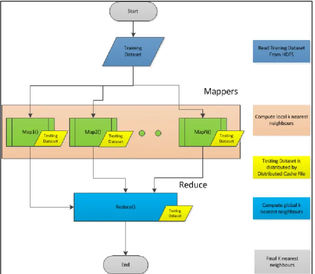
In this section we present the main design for the parallel kNN algorithm based on MapReduce. In order to transform the sequential kNN as map and reduce functions, the sequential algorithm should be analyzed to determine which part of the algorithm can or should be parallelized. In the sequential kNN algorithm, the most intensive computation is the computation of distances with neighbors. The design of the algorithm originated from a article of Processing kNN Queries in Hadoop [27]. We face another obstacle, which is the fact that two different data sets need to be fed into MapReduce: the training set and the test set (Figure 13). This problem is solved using RHadoop again, with the test set fed to each map and reduce via a distributed cache file. The kNN function is implemented as a MapReduce job comprising several Mappers and a Reducer. The overview of the map and reduce function is shown inFigure 13.
traincol<-which( colnames(data)=="A.OTHP3 ") cluster_raw<-NULL train<-matrix(data[,traincol],nrow(data),1) for(i in 1:ncol(data)){ test<-matrix(data[,i],nrow(data),1) clust<-round(nrow(data)/k,digits=0) cl <- tapply(numeric(paste(train)), k)
raw_cluster<-knn(train, test, cl$[1,], k, prob=TRUE)
Page 39 / 75
Figure 13: Flow Chart of Parallel kNN Algorithm Based on MapReduce
Map Function:
The map functions will be triggered for every training set data item, and will simply compute the Euclidean distance function. In Listing 7 as illustrated, the distances between all testing sets and training sets are calculated concurrently through computing nodes, with every node responsible for calculating the distance between all data items in the complete testing set and a subset of the training set. Then the results – which are the k-nearest local neighbors – are emitted to the reducer.
Page 40 / 75
Listing 7: Source Code of Map Function for Parallel kNN Algorithm Based on MapReduce
Reduce Function:
The Reduce function will take every testing data item and all its neighbors (local neighbors) in Listing 8. It will then sort all the neighbors in ascending order based on the distance, and will select the K nearest neighbors (global neighbors) from the list. The output of the kNN Reduce function contains the classification prediction of the entire testing set. It is stored in HDFS.
Listing 8: Source Code of Reduce Function for Parallel kNN Algorithm Based on MapReduce
5.3.3. Clustering Module
This section presents the implementation of the K-means function in three different ways: sequential, parallel based on multi-core, and parallel based on MapReduce.
5.3.3.1. Sequential:
In order to implement the k-means function, the simple stats R package and its k-means function are used in Listing 9 as follows:
map<-function(x,p){
x=t(matrix(x,length(x),length(test))) # form a matrix of train columns test.dist=matrix(test,length(test),ncol(x)) # form a test matrix accordingly dist=sqrt((x-test.dist)^2) # compute distance
temp=apply(dist,1,sort) # sort local distances temp=t(temp) # transpose it
temp=temp[,1:k] # taking lowest k distances P=matrix(p,length(test)) # key matrix
keyval=cbind(P,temp) # combining key with values}
reduce<-function(x,P){# reduce function with key and values
reduce.out=apply(map.out,1,sort) # sort all local distance after combining as global reduce.out=reduce.out[,1:k] # taking first k minimum global distances
reduce.out[which(reduce.out[,1: