Abstract—Super-resolution mapping (SRM) is a commonly used method to cope with the problem of mixed pixels when predicting the spatial distribution within low-resolution pixels. Central to the popular SRM method is the spatial pattern model, which is utilized to represent the land cover spatial distribution within mixed pixels. The use of an inappropriate spatial pattern model limits such SRM analyses. Alternative approaches, such as deep-learning-based algorithms, which learn the spatial pattern from training data through a convolutional neural network, have been shown to have considerable potential. Deep learning methods, however, are limited by issues such as the way the fraction images are utilized. Here, a novel SRM model based on a generative adversarial network (GAN), GAN-SRM, is proposed that uses an end-to-end network to address the main limitations of existing SRM methods. The potential of the proposed GAN-SRM model was assessed using four land cover subsets and compared to hard classification and several popular SRM methods. Experimental results show that of the set of methods explored, the GAN-SRM model was able to generate the most accurate high-resolution land cover maps.
Index Terms—Super-resolution mapping, deep learning, generative adversarial network
I. INTRODUCTION
HE problem of mixed pixels is commonly encountered during the process in the interpretation of remotely sensed imagery [1]. Soft classification estimates fraction values of all land cover classes within low-resolution pixels. However, it does not indicate their spatial distribution [2]. SRM may further predict the spatial distribution within the subpixels and yield a resultant high-resolution land cover map from the intermediate output of soft classification or from remotely sensed imagery directly [3, 4]. SRM has been widely applied in the geographical fields and shown to be prospective in the analysis of the mixed pixels problem [5, 6].
SRM techniques can roughly be classified into two categories, mainly according to the process representing the land cover spatial distribution. The first category describes land
This work was supported in part by Innovation Group Project of Hubei Natural Science Foundation (2019CFA019), in part by the Hubei Province Natural Science Fund for Distinguished Young Scholars (Grant No. 2018CFA062), in part by the Natural Science Foundation of China (Grant No. 61671425), and in part by the Youth Innovation Promotion Association CAS (2017384). (Corresponding author: Xiaodong Li, email: [email protected])
C. Shang, X. Li, Y. Du, and F. Ling are with the Key laboratory of Monitoring and Estimate for Environment and Disaster of Hubei province, Innovation Academy for Precision Measurement Science and Technology, Chinese Academy of Sciences, Wuhan 430077, P.R. China.
G. Foody is with School of Geography, University of Nottingham, University Park, Nottingham NG7 2RD, U.K.
cover patterns using pre-defined prior models, such as the spatial dependence model, which can be developed at the sub-pixel scale [7], the pixel/sub-pixel scale [8], or the multiple scales [9]. These models have been widely used, but it can be challenging to appropriately model some land cover mosaics, especially in highly fragmented landscapes [10]. The second category learns the land cover spatial distribution directly from additional training samples [11]. The learning-based models learn the land cover spatial pattern directly from the training samples, and can reconstruct the land cover spatial pattern better compared with the pre-defined prior models [12].
Learning-based SRM models often comprise two steps. The first step is fraction-image super-resolution (SR), which reconstructs a high-spatial-resolution fraction image from the low input. At present, support vector regression (SVR) [13], convolutional neural network (CNN) [14], and other machine learning methods have already been widely used in the fraction-image SR task. The second step is converting the high-resolution fraction images to a categorical land cover map.
Although the two-step learning-based SRM models have shown great potential, limitations still exist. First, the information extracted from the training data is only used in the fraction-image SR step, but is not used in the step of converting the fraction images to the categorical map [15]. Since the latter step does not use any information from the training data and can be viewed as a post-processing process applied to the super-resolved fraction images, the existing two-step learning-based SRM models, such as CNN-based [14], are not end-to-end. Second, the conversion step of the fraction images to the categorical map usually contains a large uncertainty. For instance, the softmax function was used in [16] to assign each high-resolution pixel to a unique category value, while optimization algorithms, such as the simulated annealing algorithm [17] and the linear optimization model [14], are used in the conversion of the fraction images to the categorical map so that the class fractions in the input low-resolution fraction image and the resultant high-resolution categorical map are unchanged. Different methods used in the conversion of the fraction images to the categorical map step will generate different SRM results [14,16-17]. The uncertainty is especially large when the high-resolution class fractions of different classes are close or equal and when the scale factor is large [14].
In this letter, an end-to-end SRM model based on a generative adversarial network (GAN), i.e., GAN-SRM, is proposed to improve the current two-step learning based SRM methods. GAN has shown more potential than other CNN based approaches in image SR [18], but to our knowledge, it has not been used in SRM. In the proposed GAN-SRM model,
Super-resolution land cover mapping using a
generative adversarial network
Cheng Shang, Xiaodong Li, Giles Foody, Fellow, IEEE, Yun Du, Feng Ling
II. METHODOLOGY
A. GAN-SRM Description
Suppose the low-resolution fraction image F has been generated by soft classification from the original remotely sensed image. This input fraction image F has ijc pixels, whose the number of land cover classes is c. It is assumed the zoom factor is z, each low-resolution pixel from F is divided into z2 high-resolution subpixels, and these all target high-resolution subpixels are considered to be assigned to a unique land cover class from c. The goal of GAN-SRM is to produce a high-resolution land cover map M with a size of (i·z)(j·z)1 using F as input.
N pairs of training datasets are available during the training procedure. Each pair contains a low-resolution class fraction image L and corresponding high-resolution land cover map H. The GAN-SRM should be first trained to model the relationship between L and H. Once the GAN-SRM model is trained, it can then be used to generate M from F.
B. FISRGAN (fraction-image SR using GAN)
In general, FISRGAN consists of two adversarial models: a generative network G and a discriminative network D [19]. The goal of FISRGAN is to train G to generate a high-resolution fraction image from a low input. At the same time, D seeks to help G to reconstruct spatial details by distinguishing real high-resolution fraction images drawn from training datasets and fake images estimated from G [20]. More details about SRGAN architecture and training procedures are introduced in [18] and [19].
To achieve this goal, the training procedure is performed on G and D iteratively for solving the two-player min-max game with a value function [21]:
input image x from pX(x). Here, the training dataset that includes pX(x) and pY(y) is available, and y is the high version of its low-resolution image x.
At the same time, D is further trained.D takes an image as input stochastically chosen to be either G(x) produced by G, or y drawn from the pY(y), and outputs a scalar probability D(G(x)) or D(y). The probability is set to between 0 and 1, which is high (close to 1) if the input was y and low (close to 0) if the input was G(x). Then this probability will be used to guide the optimization of G. In other words, the discriminative network is a magistrate of the generative network [19].
C. GAN-SRM Network Architecture
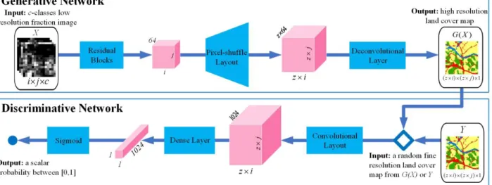
The proposed GAN-SRM model also includes a generative network G and a discriminative network D (Fig. 1).
1) The Generative Network G
The input to the generative network G is a c-classes low-resolution fraction image with the size of ijc, and the output is a high-resolution land cover map with the size of (i·z)(j·z)1. G includes a residual block, a pixel-shuffle layout, and a deconvolutional layer.
In this letter, a selected part of layers from [18], which include residual blocks and a pixel-shuffle layout, are used. The residual block aims to convolute the c-class fraction values to a one-strided channel through 64 feature maps. The pixel-shuffle layout is used for upsampling the feature maps [22]. According to the FISRGAN, the cores of the residual block and pixel-shuffle layout are conventional CNNs. Additional details can be obtained in Fig. 1, Fig. 2 (a-b) and [18].
With FISRGAN, the output is not the expected land cover map but the fraction images. A deconvolutional layer is further modeled to learn the nonlinear relationship between fraction values and class labels, which has already been shown to an effective technique for data-type transformation in [23].
Employing the same operation, the expected one-channel (i·z)(j·z) high-resolution land cover map can be estimated by compressing the feature maps to one dimension and normalizing the fraction values into a unique discrete land cover class labels from c.
2) The Discriminative Network D
Once G has been trained, it can be used for SRM. However, the ill-posed nature of the SR problem is still pronounced. Thus the discriminative network D is designed to tackle the ill-posed drawbacks, which aims to distinguish real and generated land cover maps through recovering spatial details. The input of the D is an (i·z)(j·z) land cover map stochastically chosen from the training dataset or the generative network, and the output is a scalar probability. D includes a convolutional layout, a dense layer, and a final sigmoid function (Fig. 1 and Fig. 2 (c)). A convolutional layout is firstly employed to feature extraction. After extraction, a dense layer is used to further reduces the dimensions of land cover feature maps. Finally, a sigmoid function is used to constrain the dense to a scalar value between 0 and 1, which will guide to optimize the generative network.
3) Loss function of GAN-SRM
In GAN-SRM, the generalized loss function in equation (1) is re-written as the sum of a generative loss (LossMSE) and an adversarial loss (LossProbability) as:
{
Generative loss calculated based on MSE Adversarial loss calculated based on Probability to capture pixel-wise differences to capture high-frequency differences
total MSE Pr obability
Loss = Loss + Loss
1442 443
(2)The generative loss aims to assess the pixel-wise similarity between the generated and real land cover maps, which is calculated as: MSE 2 2 1 1 , 1 ( ( ) ) zi zj G i j i j Loss H G L z ij = = =
− (3)where GθG is the generative network parameterized by the
weights and biases θG. Here, θG is obtained by solving the generative loss function in equation (3). The optimization target of generative loss based on pixel-wise is the minimization of the mean squared error (MSE), which is calculated between the generated GθG(L) and real H [24].
Given that fraction-image SR and the conversion of the fraction images to the categorical map steps are intended to train in one generative network simultaneously, the computational burden of the target is cumbersome, and the ability of generative loss to capture high-frequency differences is minimal. Thus, the high-frequency spatial details cannot be thoroughly recovered by calculating a single generative loss. An adversarial loss is then further designed to favor solutions that reside on the high-frequency details, which is the most
considerable improvement in contrast to existing CNN. The adversarial loss is calculated as negative log-likelihood loss as:
1 log D( G( )) N Probability n Loss D G L = =
− (4) where DθD is the discriminative network parameterized by theweights and biases θD. Here, θD is obtained by solving the adversarial loss function in equation (4). The adversarial loss is calculated based on the probability DθD(GθG(L)), which is used to
decide whether the generated map GθG(L) is real or generated.
III. EXPERIMENTS
A. Dataset
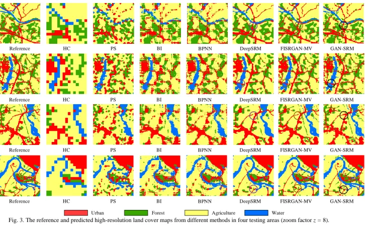
The proposed model was explored using subset test maps and training datasets extracted from the National Land Cover Database (NLCD) obtained from Landsat with 16 land cover classes [13]. The elementary classes of NLCD were summarized into four typical classes: forest, urban, agriculture, and water. The methods were validated using four maps with 120120 pixels in Fig. 3. For each map, the synthetic low-resolution fraction images were produced by linear averaging the original land cover map with a zoom factor z=8. B. Model Implementation
In the initialization step, the hyper-parameters of GAN-SRM are set manually. The initial learning-rate was 0.001, the mini-batch was 32, and the number of the iteration was 2000. The whole model was trained by an Adam optimizer. All weights and biases of θG and θD were randomly initialized by a zero-centered normal distribution, whose standard deviation is 0.02. The work was undertaken on TensorFlow 2.0 with an NVIDIA RTX 2070 Super GPU.
During the training process of the mini-batch, the parameters θD will be obtained when GθG is first trained. In each inner loop,
DθD is then updated by one real case and one generated case of
random inputs. In the real case, the parameters θD are updated by setting the output probability to be 1. In the generated case, the parameters θD are updated by setting the output probability to be 0. Thus, this convergence process will emerge a gradient
∇, which will guide GθG again to produce more accurate
high-resolution land cover maps by backpropagation. The same procedure for renewing θG and θD is repeated. The iteration terminates when the constant Losstotal in equation (2) is obtained, or the predetermined iteration times are reached. C. Comparison Methods
The proposed GAN-SRM was evaluated by comparing with a pixel-based method of hard classification (HC), as well as
Fig. 2. Detailed architecture of a) the residual blocks, b) the pixel-shuffle layout, and c) the convolutional layout with corresponding kernel size (k), number of feature maps (n) and stride (s) indicated for each convolutional layer.
was first used to downscale the low-resolution fraction images to a high-resolution scale, and then the pixel label for each fine-resolution pixel was assigned to the class with the maximal fraction value in that pixel. For the learning-base SRMs, 900 subsets maps of NLCD (each containing 400400pixels) and the corresponding fraction images were used to form the required training dataset. By comparing different SRMs with the reference maps in Fig. 3, the overall accuracy (OA) was chosen for assessment.
IV. RESULTS AND DISCUSSION
The resultant high-resolution land cover maps produced from all SRMs were shown in Fig. 3. In general, SRM results based on deep-learning methods, such as DeepSRM, FISRGAN-MV, and GAN-SRM, had better performance than other algorithms. The HC results cannot represent detailed land cover features, as the spatial resolution is too low. For the results in PS, BI, and BPNN models, inter-class boundaries in the were jagged, and many linear class features were wrongly classified into round or circle patches. PS and BI use the maximum spatial dependence principle and may be inappropriate to describe the land cover pattern of linear features, and generate aggregated patches and discontinuous linear features. This is because the maximal spatial dependence
thoroughly learn the complex spatial information.
In comparison, DeepSRM, FISRGAN-MV, and GAN-SRM are convolutional networks-based methods. Many isolated land cover patches and jagged shapes were found in the DeepSRM and FISRGAN-MV maps. For instance, the linear urban pieces were disconnected (as are highlighted in the purple and brown circle in Fig. 3). In contrast, details produced by GAN-SRM were better reconstructed, and the linear urban patches (as are also highlighted in the black circle in Fig. 3) were more connected. This improvement arises based on two aspects. First, the architecture of DeepSRM is a CNN with 21 convolutional layers [14], which only calculates MSE loss function by reconstructs purely pixel-wise differences, while the two methods using GAN add an extra adversarial loss function to capture high-frequency differences. As a result, the performance of reconstructing high details in GAN (with discriminative network and adversarial training) is better than the CNN. Second, both DeepSRM and FISRGAN-MV are two-step approaches. The information from the training data is only used in the fraction-image SR but not in the conversion of the fraction images to the categorical map step. Therefore, the latter step in DeepSRM and FISRGAN-MV generated isolated patches and jagged shapes that were dissimilar to the reference. In contrast, GAN-SRM adopts a novel end-to-end architecture
I II III IV HC PS BI BPNN DeepSRM FISRGAN-MV Reference GAN-SRM HC PS BI BPNN DeepSRM FISRGAN-MV Reference GAN-SRM HC PS BI BPNN DeepSRM FISRGAN-MV Reference GAN-SRM HC PS BI BPNN DeepSRM FISRGAN-MV Reference GAN-SRM
Urban Forest Agriculture Water
Fig. 3. The reference and predicted high-resolution land cover maps from different methods in four testing areas (zoom factor z = 8). Each area contains 120 120 pixels and four land cover classes.
and fully considers the spatial distribution for discrete land cover class labels through the deconvolutional layer, and generate land cover maps that are the most similar to the reference maps in Fig. 3.
Table 1 illustrates the quantitative result of different methods. The OA of HC, PS, BI, and BPNN, are lower than those obtained by SRM methods based on deep-learning, such as DeepSRM, FISRGAN-MV, and GAN-SRM. Furthermore, the OA of GAN-SRM is the highest, highlighting the advantage of the proposed approach.
V. CONCLUSION
In this letter, a novel end-to-end GAN-SRM model is proposed for super-resolution land cover mapping. In the proposed model, fraction-image SR and the conversion of the fraction images to the categorical map steps are integrated into one generative network. A discriminative network is further trained and plays an adversarial role to optimize the generative network to model a nonlinear function between the low-resolution fraction images and high-resolution land cover categorical maps. The performance of the proposed GAN-SRM algorithm was validated with several test maps, and was compared with popular PS, BI, BPNN, DeepSRM, and adjusted FISRGAN-MV methods. The experimental results showed that the GAN-SRM model was superior to other comparing SRMs not only in terms of the OA but also visually. In comparison to the other SRMs, the resultant high-resolution land cover maps from GAN-SRM provided a superior representation of class distributions by restoring more high-frequency details.
REFERENCES
[1] P. M. ATKINSON, “Issues of uncertainty in super-resolution mapping and their implications for the design of an inter-comparison study,”
International Journal of Remote Sensing, vol. 30, no. 20, pp. 5293-5308, 2009.
[2] G. M. Foody, “The role of soft classification techniques in the refinement of estimates of ground control point location,” Photogrammetric Engineering and Remote Sensing, vol. 68, no. 9, pp. 897-904, 2002. [3] Y. Ge, Y. Chen, S. Li, and Y. Jiang, “Vectorial boundary-based sub-pixel
mapping method for remote-sensing imagery,” International Journal of Remote Sensing, vol. 35, no. 5, pp. 1756-1768, 2014.
[4] Y. Zhang, Y. Du, F. Ling, and X. Li, “Improvement of the Example-Regression-Based Super-Resolution Land Cover Mapping Algorithm,” IEEE Geoscience & Remote Sensing Letters, vol. 12, no. 8, pp. 1740-1744, 2015.
[5] F. Ling, D. Boyd, Y. Ge, G. M. Foody, X. Li, L. Wang, Y. Zhang, L. Shi, C. Shang, and X. Li, “Measuring River Wetted Width from Remotely Sensed Imagery at the Sub‐pixel Scale with a Deep Convolutional Neural Network,” Water Resources Research, vol. 55, no. 7, pp. 5631-5649, 2019.
[6] G. M. Foody, A. M. Muslim, and P. M. Atkinson, “Super‐resolution mapping of the waterline from remotely sensed data,” International Journal of Remote Sensing, vol. 26, no. 24, pp. 5381-5392, 2005.
[7] P. M. Atkinson, “Sub-pixel Target Mapping from Soft-classified, Remotely Sensed Imagery,” Photogrammetric Engineering & Remote Sensing, vol. 71, no. 7, pp. 839-846, 2005.
[8] K. C. Mertens, B. D. Baets, L. P. C. Verbeke, and R. R. D. Wulf, “A sub‐pixel mapping algorithm based on sub‐pixel/pixel spatial attraction models,” International Journal of Remote Sensing, vol. 27, no. 15, pp. 3293-3310, 2006.
[9] F. Ling, Y. Du, L. Xiaodong, Y. Zhang, F. Xiao, S. Fang, and W. Li, “Superresolution Land Cover Mapping With Multiscale Information by Fusing Local Smoothness Prior and Downscaled Coarse Fractions,” IEEE Transactions on Geoscience & Remote Sensing, vol. 52, no. 9, pp. 5677-5692, 2014.
[10] Y. Ge, S. Li, and V. C. Lakhan, “Development and Testing of a Subpixel Mapping Algorithm,” IEEE Transactions on Geoscience & Remote Sensing, vol. 47, no. 7, pp. 2155-2164, 2014.
[11] X. Li, F. Ling, G. M. Foody, Y. Ge, Y. Zhang, and Y. Du, “Generating a series of fine spatial and temporal resolution land cover maps by fusing coarse spatial resolution remotely sensed images and fine spatial resolution land cover maps,” Remote Sensing of Environment, vol. 196, pp. 293-311, 2017.
[12] Y. Ge, Y. Chen, S. Alfred, S. Li, and J. Hu, “Enhanced Subpixel Mapping With Spatial Distribution Patterns of Geographical Objects,” IEEE Transactions on Geoscience & Remote Sensing, vol. 54, no. 4, pp. 1-15, 2016.
[13] Y. Zhang, D. Yun, L. Feng, S. Fang, and X. Li, “Example-Based Super-Resolution Land Cover Mapping Using Support Vector Regression,” IEEE Journal of Selected Topics in Applied Earth Observations & Remote Sensing, vol. 7, no. 4, pp. 1271-1283, 2014. [14] F. Ling, and G. M. Foody, “Super-resolution land cover mapping by deep
learning,” Remote Sensing Letters, vol. 10, no. 6, pp. 598-606, 2019. [15] Y. Makido, A. Shortridge, and J. P. Messina, “Assessing Alternatives for
Modeling the Spatial Distribution of Multiple Land-cover Classes at Sub-pixel Scales,” Photogrammetric Engineering & Remote Sensing, vol. 73, no. 8, pp. 935-943, 2007.
[16] Y. Jia, Y. Ge, Y. Chen, S. Li, G. Heuvelink, and F. Ling, “Super-resolution land cover mapping based on the convolutional neural network,” Remote Sensing, vol. 11, no. 15, pp. 1815, 2019.
[17] F. Ling, Z. Yihang, G. M. Foody, L. Xiaodong, and Y. Du, “Learning-Based Superresolution Land Cover Mapping,” IEEE Transactions on Geoscience & Remote Sensing, vol. 54, no. 7, pp. 1-17, 2016.
[18] C. Ledig, L. Theis, F. Huszar, J. Caballero, A. Cunningham, A. Acosta, A. Aitken, A. Tejani, J. Totz, and Z. Wang, “Photo-Realistic Single Image Super-Resolution Using a Generative Adversarial Network,” 2017 IEEE Conference on Computer Vision and Pattern Recognition (CVPR), pp. 4681-4690, 2016.
[19] I. Goodfellow, J. Pouget-Abadie, M. Mirza, B. Xu, D. Warde-Farley, S. Ozair, A. Courville, and Y. Bengio, “Generative adversarial nets,”
Proceedings of the 27th International Conference on Neural Information Processing Systems, vol. 2, pp. 2672-2680, 2014.
[20] X. Wang, K. Yu, S. Wu, J. Gu, Y. Liu, C. Dong, Y. Qiao, and C. C. Loy, “ESRGAN: Enhanced Super-Resolution Generative Adversarial Networks,” European Conference on Computer Vision, pp. 63-70, 2018. [21] K. Lata, M. Dave, and K. N. Nishanth, “Image-to-Image Translation
Using Generative Adversarial Network,” 2019 3rd International Conference on Electronics, Communication and Aerospace Technology (ICECA), 2019.
[22] W. Shi, J. Caballero, F. Huszár, J. Totz, and Z. Wang, “Real-Time Single Image and Video Super-Resolution Using an Efficient Sub-Pixel Convolutional Neural Network,” Journal, Year.
[23] M. D. Zeiler, D. Krishnan, G. W. Taylor, and R. Fergus, “Deconvolutional networks,” IEEE Computer Society Conference on Computer Vision and Pattern Recognition, 2010.
[24] S. Saha, F. Bovolo, and L. Bruzzone, “Unsupervised Multiple-Change Detection in VHR Multisensor Images Via Deep-Learning Based Adaptation,” IGARSS 2019-2019 IEEE International Geoscience and Remote Sensing Symposium, pp. 5033-5036, 2019.
[25] L. Feng, D. Yun, X. Li, W. Li, X. Fei, and Y. Zhang, “Interpolation-based super-resolution land cover mapping,” Remote Sensing Letters, vol. 4, no. 7, pp. 629-638, 2013.
[26] L. Zhang, W. Ke, Y. Zhong, and P. Li, “A new sub-pixel mapping algorithm based on a BP neural network with an observation model,”
Neurocomputing, vol. 71, no. 10, pp. 2046-2054, 2008. TABLEI
OVERALL ACCURACY OF LAND COVER MAPS BY DIFFERENT METHODS Test Map HC PS BI BP DeepSRM FISRGAN-MV GAN_SRM
I 69.57 68.06 70.54 71.24 74.19 81.63 84.27
II 67.91 63.85 68.72 68.01 75.55 77.41 79.89
III 76.90 75.90 78.53 78.52 83.70 84.51 86.25