Project September 2008

(1)

MEASURING THE BENEFITS OF

IMPLEMENTING ASSET

MANAGEMENT SYSTEMS AND

TOOLS

Project 06-06

September 2008

Midwest Regional University Transportation Center

College of Engineering

Department of Civil and Environmental Engineering

University of Wisconsin, Madison

Authors: Sue McNeil, and Daisuke Mizusawa

University of Delaware and Urban Transportation Center, University of Illinois-Chicago

Principal Investigator: Dr. Sue McNeil;

Professor, University of Delaware, and Adjunct Professor, Urban Transportation Center,

University of Illinois, Chicago

(2)

DISCLAIMER

This research was funded by the Midwest Regional University Transportation Center. The contents of this report reflect the views of the authors, who are responsible for the facts and the accuracy of the information presented herein. This document is disseminated under the

sponsorship of the Department of Transportation, University Transportation Centers Program, in the interest of information exchange. The U.S. Government assumes no liability for the contents or use thereof. The contents do not necessarily reflect the official views of the Midwest

Regional University Transportation Center, the University of Wisconsin, the Wisconsin Department of Transportation, or the USDOT’s RITA at the time of publication.

The United States Government assumes no liability for its contents or use thereof. This report does not constitute a standard, specification, or regulation.

The United States Government does not endorse products or manufacturers. Trade and manufacturers names appear in this report only because they are considered essential to the object of the document.

(3)

Technical Report Documentation Page

1. Report No. 2. Government Accession No. 3. Recipient’s Catalog No.

4. Title and Subtitle

Measuring the Benefits of Implementing Asset Management Systems and Tools

5. Report Date September 19, 2008 6. Performing Organization Code

7. Author/s Sue McNeil, and Daisuke Mizusawa _{8. Performing Organization Report No.}

MRUTC 06-06 9. Performing Organization Name and Address

Midwest Regional University Transportation Center University of Wisconsin-Madison

1415 Engineering Drive, Madison, WI 53706

10. Work Unit No. (TRAIS) 11. Contract or Grant No. DTRS 99-G-0005 12. Sponsoring Organization Name and Address

Research and Innovative Technology Administration U.S. Department of Transportation

1200 New Jersey Avenue, SE Washington, D.C. 20590

13. Type of Report and Period Covered Research Report

June 2005 – September 2008 14. Sponsoring Agency Code

15. Supplementary Notes Project completed for the Midwest Regional University Transportation Center with support from the Wisconsin Department of Transportation and Metropolitan Transportation Support Inistiave (METSI) at University of Illinois at Chicago.

16. Abstract

Although transportation agencies in the U.S. have been developing Asset Management Systems (AMS) for specific types of infrastructure assets, there are several barriers to the

implementation of AMS. In particular, implementation and development costs are critical issues. Without showing that AMS implementation improves asset performance and that the benefits of AMS implementation outweigh the costs for AMS implementation and operation, further implementation and development will not occur. This paper documents the development of a generic methodology for quantifying the benefits derived from implementation of AMS and justifying investment in AMS implementation. The generic methodology involves three analysis methods: descriptive analysis, regression analysis, and benefit-cost analysis. These methods draw on basic principles of engineering economic analysis and apply to two types of evaluations: an ex post facto evaluation and an ex ante evaluation depending on the time frame and the availability of time series data. While the concepts are relatively simple, the challenge lies in identifying data to support the application of the methodology. This paper demonstrates how the methodology can be applied to evaluate the implementation of a pavement

management system in terms of efficacy, effectiveness, and efficiency (3Es). 17. Key Words

Asset Management, Benefits

18. Distribution Statement

No restrictions. This report is available through the Transportation Research Information Services of the National Transportation Library.

19. Security Classification (of this report)

Unclassified 20. Security Classification (of this page) Unclassified 21. No. Of Pages 186 22. Price -0-

(4)

LIST OF TABLES

TABLE 1.BENEFITSANDCOSTS ... 7

TABLE 2.COMPARISONOFTWAPC ... 12

TABLE 3.ASSETMANAGEMENTSYSTEMSREQUIREDBYISTEA ... 23

TABLE 4.LISTOFALTERNATIVESINBENEFITQUANTIFICATION ... 39

TABLE 5. BENEFITSANDCOSTSINBENEFITQUANTIFICATION ... 40

TABLE 6.INTERPRETATIONOFRESULTS ... 42

TABLE 7.LISTOFALTERNATIVEININVESTMENTJUSTIFICATION ... 42

TABLE 8.BENEFITSANDCOSTSININVESTMENTJUSTIFICATOIN ... 43

TABLE 9.ROADNETWORKCONDITIONIN2006 ... 51

TABLE 10. DATAFORREGRESSIONANALYSIS ... 54

TABLE 11.MEANSOFAVERAGEPAVEMENTCONDITIONOVER14YEARS ... 56

TABLE 12.MEANOFPERCENTTRAVELBYPAVEMENTCONDITIONOVER14YEARS ... 59

TABLE 13.PERFORMANCEWITHPMS ... 60

TABLE 14.PERFORMANCEWITHOUTPMS ... 61

TABLE 15.VALUEOFIMPROVEMENTINEFFECTIVENESS ... 62

TABLE 16. HIGHWAYNETWORKCONDITIONINHPMSDATA ... 68

TABLE 17.DEFICIENCYCRITERIAINPSR ... 69

TABLE 18.PAVEMENTCONDITIONRATINGS ... 72

TABLE 19.NUMBERSOFSECTIONSANDSELECTEDSECTIONS ... 73

TABLE 20. LENGTHSOFSECTIONSANDSELECTEDSECTIONS(LANE-MILES) ... 73

TABLE 21. LENGTHSOFSELECTEDSECTIONSFORAWORSTFIRSTSTRATEGY (LANE-MILES) ... 73

TABLE 22. NUMBERSOFSECTIONSANDSELECTEDSECTIONSFORSECONDPERIOD ... 74

TABLE 23.LENGTHSOFSECTIONSANDSELECTEDSECTIONSFORSECONDPERIOD (LANE-MILES) ... 74

TABLE 24.LENGTHSOFSELECTEDSECTIONSFORAWORSTFIRSTSTRATEGYIN SECONDPERIOD(LANE-MILES) ... 74

TABLE 25.RESPONSESINCOMPARISONOFINITIALCOSTS ... 75

TABLE 26. DATAFORREGRESSIONANALYSIS ... 77

TABLE 27.INITIALCOSTSOFWITHANDWITHOUTHERS-STCASES ... 79

TABLE 28. MEANSOFTRAFFICWEIGHTEDAVERAGEPAVEMNETCONDITIONOVER 10YEARS ... 79

TABLE 29. MEANOFPERCENTTRAVELBYPAVEMENTCONDITIONOVER10YEARS ... 82

TABLE 30. WITHANDWITHOUTPERFORMANCEMEASURES ... 86

TABLE 31. WITHANDWITHOUTSYSTEMCONDITIONS ... 88

TABLE 32. COSTSANDBENEFITSOFWITHANDWITHOUTCASES ... 92

TABLE 33. REQUIREDDATA ... 99

TABLE 34.SUMMARYOFGENERICMETHODOLOGY ... 105

TABLE 35.RESULTSOFCASESTUDIESUSINGGENERICMETHODOLOGY ... 107

TABLE 36.ALTERNATIVEMETHODSFORINFERRINGDEMANDFUNCTION ... 124

(7)

TABLE 38.ENVIRONMENTALPROBLEMSANDCAUSEDBYTRANSPORTATION

PROJECTS ... 131

TABLE 39. BENEFITSOFAMSIMPLEMENTATION ... 137

TABLE 40.COSTSOFAMSIMPLEMENTATION ... 140

(8)

LIST OF FIGURES

FIGURE 1. CONCEPTS OF EX POST FACTO AND EX ANTE EVALUATIONS ... 3

FIGURE 2.FLOW DIAGRAM ... 4

FIGURE 3.RELATIONSHIP OF ANALYSIS PERIODS ... 8

FIGURE 4.RELATIONSHIP OF ANALYSIS METHODOLOGY ... 11

FIGURE 5. CONCEPTUAL DECISION-MAKINGS BETWEEN ‘WITH’ AND ‘WITHOUT’CASES ... 14

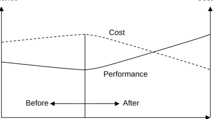
FIGURE 6.CONCEPTUAL RELATIONSHIP BETWEEN PERFORMANCE AND COST BEFORE AND AFTER IMPLEMENTING AMS ... 24

FIGURE 7.RELATIONSHIPS AMONG URBAN TRANSPORTATION PROBLEMS AND SOLUTIONS ... 26

FIGURE 9.CONCEPTS OF EX ANTE EVALUATION ... 34

FIGURE 8.CONCEPTS OF EX POST FACTO EVALUATION ... 34

FIGURE 10.SCHEMATIC ILLUSTRATION OF EFFECTIVENESS... 37

FIGURE 11.CONCEPT OF METHODOLOGY FOR QUANTIFYING BENEFITS ... 45

FIGURE 12.NUMBERS OF ELEMENTS BASED ON CONDITION ... 51

FIGURE 13.LENGTHS OF ELEMENTS BASED ON CONDITION ... 51

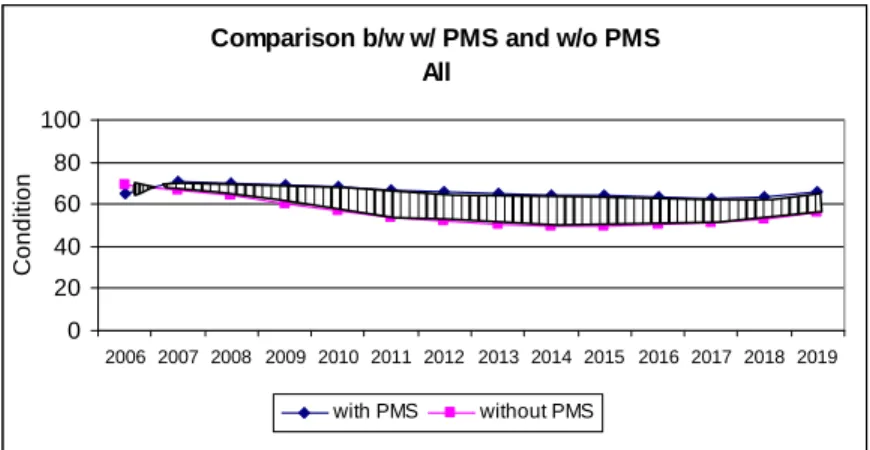
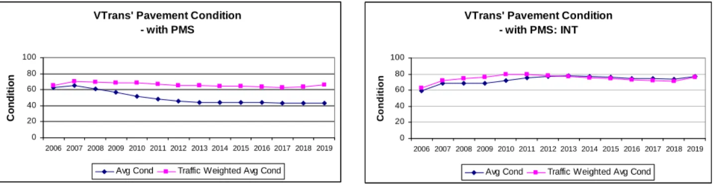
FIGURE 14.PAVEMENT CONDITION WITH PMS(ALL) ... 55

FIGURE 15.PAVEMENT CONDITION WITH PMS(INT) ... 55

FIGURE 16.PAVEMENT CONDITION WITH PMS(STE) ... 56

FIGURE 17.PAVEMENT CONDITION WITH PMS(CL1) ... 56

FIGURE 18.PAVEMENT CONDITION WITHOUT PMS(ALL) ... 56

FIGURE 19.PAVEMENT CONDITION WITHOUT PMS(INT) ... 56

FIGURE 20.PAVEMENT CONDITION WITHOUT PMS(STE) ... 56

FIGURE 21.PAVEMENT CONDITION WITHOUT PMS(CL1) ... 56

FIGURE 22.COMPARISON OF TRAFFIC WEIGHTED AVERAGE PAVEMENT CONDITIONS (ALL) ... 57

FIGURE 23.COMPARISON OF TRAFFIC WEIGHTED AVERAGE PAVEMENT CONDITIONS (INT) ... 57

FIGURE 24.COMPARISON OF TRAFFIC WEIGHTED AVERAGE PAVEMENT CONDITIONS (STE) ... 57

FIGURE 25.COMPARISON OF TRAFFIC WEIGHTED AVERAGE PAVEMENT CONDITIONS (CL1) ... 57

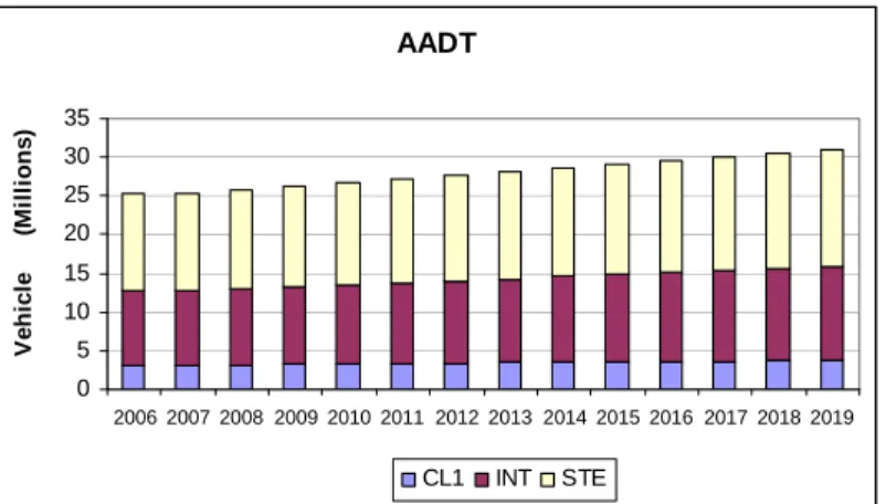
FIGURE 26.AADT BASED ON ROAD CLASS ... 58

FIGURE 27.PERCENT TRAVEL BY CONDITION WITH PMS(ALL) ... 58

FIGURE 28.PERCENT TRAVEL BY CONDITION WITH PMS(INT) ... 58

FIGURE 29.PERCENT TRAVEL BY CONDITION WITH PMS(STE) ... 58

FIGURE 30.PERCENT TRAVEL BY CONDITION WITH PMS(CL1) ... 58

FIGURE 31.PERCENT TRAVEL BY CONDITION WITHOUT PMS(ALL) ... 59

FIGURE 32.PERCENT TRAVEL BY CONDITION WITHOUT PMS(INT) ... 59

FIGURE 33.PERCENT TRAVEL BY CONDITION WITHOUT PMS(STE) ... 59

FIGURE 34.PERCENT TRAVEL BY CONDITION WITHOUT PMS(CL1) ... 59

FIGURE 35.EFFECTIVENESS (INT) ... 60

FIGURE 36.EFFECTIVENESS (ALL) ... 60

FIGURE 37.EFFECTIVENESS (CL1)... 60

FIGURE 38.EFFECTIVENESS (STE)... 60

FIGURE 39.RELATIONSHIP BETWEEN TRAFFIC WEIGHTED AVERAGE PAVEMENT CONDITION AND AADT ... 62

FIGURE 40.EXCEL OUTPUTS ... 63

FIGURE 41.HERS-ST ANALYTICAL PROCEDURES (U.S.DOT AND FHWA,2005) ... 67

(9)

FIGURE 43.LENGTHS OF HIGHWAY NETWORK IN HPMS DATA ... 68

FIGURE 44.CONCEPTS OF WITHOUT HERS-ST CASE AND WITH HERS-ST CASE ... 69

FIGURE 45.FLOW DIAGRAM OF PROCESS ... 71

FIGURE 46.SCHEMATIC ILLUSTRATION OF EFFECTIVENESS IN HERS-ST CASE ... 77

FIGURE 47.COMPARISON OF TRAFFIC WEIGHTED AVERAGE PAVEMENT CONDITIONS (ALL) ... 80

FIGURE 48.COMPARISON OF TRAFFIC WEIGHTED AVERAGE PAVEMENT CONDITIONS (RURAL PRINCIPAL) ... 80

FIGURE 49.COMPARISON OF TRAFFIC WEIGHTED AVERAGE PAVEMENT CONDITIONS (RURAL MINOR) ... 80

FIGURE 50.COMPARISON OF TRAFFIC WEIGHTED AVERAGE PAVEMENT CONDITIONS (URBAN PRINCIPAL) ... 80

FIGURE 51.PERCENT TRAVEL BY CONDITION WITH HERS-ST(ALL) ... 81

FIGURE 52.PERCENT BY TRAVEL BY CONDITION WITH HERS-ST(RURAL PRINCIPAL) ... 81

FIGURE 53.PERCENT TRAVEL BY CONDITION WITH HERS-ST (RURAL MINOR) ... 81

FIGURE 54.PERCENT TRAVEL BY CONDITION WITH HERS-ST(URBAN PRINCIPAL) ... 81

FIGURE 55.PERCENT TRAVEL BY CONDITION WITHOUT HERS-ST(ALL) ... 81

FIGURE 56.PERCENT TRAVEL BY CONDITION WITHOUT HERS-ST(RURAL PRINCIPAL) ... 81

FIGURE 57.PERCENT TRAVEL BY CONDITION WITHOUT HERS-ST(RURAL MINOR) ... 82

FIGURE 58.PERCENT TRAVEL BY CONDITION WITHOUT HERS-ST(URBAN PRINCIPAL) ... 82

FIGURE 59.AADT OF WITH HERS-ST CASE ... 83

FIGURE 60.AADT OF WITHOUT HERS-ST CASE ... 83

FIGURE 61.TREATMENTS OF FP1 WITH HERS-ST(NUMBER OF SECTIONS) ... 84

FIGURE 62.TREATMENTS OF FP2 WITH HERS-ST(NUMBER OF SECTIONS) ... 84

FIGURE 63.TREATMENTS OF FP1 WITH HERS-ST(LANE-MILES) ... 84

FIGURE 64.TREATMENTS OF FP2 WITH HERS-ST(LANE-MILES) ... 84

FIGURE 65.TREATMENTS OF FP1 WITHOUT HERS-ST(NUMBER OF SECTIONS) ... 85

FIGURE 66.TREATMENTS OF FP2 WITHOUT HERS-ST(NUMBER OF SECTIONS) ... 85

FIGURE 67.TREATMENTS OF FP1 WITHOUT HERS-ST(LANE-MILES) ... 85

FIGURE 68.TREATMENTS OF FP2 WITHOUT HERS-ST(LANE-MILES) ... 85

FIGURE 69.PRODUCTS OF PSR,AADT, LANE, AND LENGTH OF WITH HERS-ST CASE AND WITHOUT HERS-ST CASE ... 89

FIGURE 70.RELATIONSHIP BETWEEN TRAFFIC WEIGHTED AVERAGE PAVEMENT CONDITION AND AADT ... 90

FIGURE 71.CONCEPTUAL BENEFITS OF HERS-ST IMPLEMENTATION ... 93

FIGURE 72.DATA USED BY HERS-ST WITH RESPECT TO VALUATION COMPONENTS AND MODELS 98 FIGURE 73.FLOW DIAGRAM ... 101

FIGURE 74.PREDICTED PERFORMANCES WITH AND WITHOUT AMS BASED ON EX ANTE EVALUATION ... 102

FIGURE 75.RELATIONSHIP BETWEEN EFFECTS OF AMS IMPLEMENTATION AND IMPACTS OF INFLUENCES ... 103

FIGURE 76.CONCEPTUAL PERFORMANCE AT A SECTION LEVEL ... 104

FIGURE 77.PARETO AND POTENTIAL PARETO EFFICIENCY ... 121

FIGURE 78.KALDOR-HICKS AND PARETO ... 122

FIGURE 79.DEMAND FUNCTION ... 123

FIGURE 80.USER COST FUNCTION ... 126

(10)

FIGURE 82.DEMAND FUNCTION AND CONSUMER SURPLUS ... 129

FIGURE 83.SUPPLY FUNCTION AND PRODUCER SURPLUS ... 130

FIGURE 84.CONCEPTUAL RELATIONSHIP BETWEEN VMT AND COSTS ... 131

FIGURE 85.EFFECT OF MITIGATION ... 132

FIGURE 86.USER BENEFITS ... 133

FIGURE 87.AGENCY BENEFITS ... 134

FIGURE 88.RESEARCH BASED ON BENEFITS QUANTIFICATION METHODOLOGY ... 141

FIGURE 89.PERCENT LENGTH BY CONDITION WITH PMS(ALL) ... 169

FIGURE 90.PERCENT LENGTH BY CONDITION WITH PMS(INT) ... 169

FIGURE 91.PERCENT LENGTH BY CONDITION WITH PMS(STE) ... 169

FIGURE 92.PERCENT LENGTH BY CONDITION WITH PMS(CL1) ... 169

FIGURE 93.PERCENT LENGTH BY CONDITION WITHOUT PMS(ALL) ... 170

FIGURE 94.PERCENT LENGTH BY CONDITION WITHOUT PMS(INT) ... 170

FIGURE 95.PERCENT LENGTH BY CONDITION WITHOUT PMS(STE) ... 170

(11)

LIST OF ABBREVIATIONS

AADT Annual Average Daily Traffic

AASHTO American Association of State Highway and Transportation Officials AHS Automated Highway System

ALS Area Licensing Scheme AMS Asset Management Systems APC Average Pavement Condition AVL Automated Vehicle Location

BCA Benefit-Cost Analysis BCR Benefit-Cost Ratio BHI Bridge Health Index

BMS Bridge Management Systems CMP Pavement Composite Index

dTIMS™ CT Deighton Total Infrastructure Management System DOT Department of Transportation

ESAL Equivalent Single Axle Loads ETC Electronic Toll Collection FHWA Federal Highway Administration FRT First Registration Tax

GASB Governmental Accounting Standard Board Statement GIS Geographic Information System

GLS Generalized Least Squares

HDM Highway Design and Maintenance Standard Model HERS-ST Highway Economic Requirement System – State Version HPMS Highway Performance Monitoring System

ISTEA Intermodal Surface Transportation Efficiency Act ITS Intelligent Transportation Systems

IRI International Roughness Index IRR Internal Rate of Return LRT Light Rail Transit

LTAP Local Technical Assistance Programs

M&R Maintenance and Rehabilitation NPV Net Present Value

(12)

LIST OF ABBREVIATIONS (CONTINUED)

OECD Organisation for Economic Co-operation and Development OLS Ordinary Least Squares

OMB Office of Management and Budget PCI Pavement Condition Index

PIARC World Road Association PMS Pavement Management Systems PSR Pavement Serviceability Rating PQI Pavement Quality Index

SSM Soft Systems Methodology STIP Statewide Transportation Improvement Plan TFP Total Factor Productivity

TRB Transportation Research Board

TWAPC Traffic Weighted Average Pavement Condition VKT Vehicle Kilometers Traveled

VMT Vehicle Miles Traveled VTrans Vermont Agency of Transportation

(13)

EXECUTIVE SUMMARY

Although transportation agencies in the U.S. have been developing Asset Management Systems (AMS) for specific types of infrastructure assets, there are several barriers to the

implementation of AMS. In particular, implementation and development costs are critical issues. Without evidence of AMS benefits, further implementation and development of AMS may be constrained. This research report documents the development of a generic methodology for quantifying the benefits derived from implementation of AMS and justifying investment in AMS implementation. The generic methodology involves three analysis methods: descriptive analysis, regression analysis, and benefit-cost analysis. These methods draw on basic principles of

engineering economic analysis and apply to two types of evaluations: an ex post facto evaluation

and an ex ante evaluation depending on the time frame and the availability of time series data.

While the concepts are relatively simple, the challenge lies in identifying data to support the application of the methodology. This research demonstrates how the methodology can be applied to evaluate the implementation of a pavement management system in terms of efficacy, effectiveness, and efficiency (3Es).

1. Introduction

Asset management systems (AMS) are tools designed to support the systematic process of cost-effectively maintaining, upgrading, and operating physical assets. Such systems include asset inventory, condition assessment and performance modeling, alternative selection and evaluation of maintenance and rehabilitation strategies, methods for evaluating the effectiveness of each strategy, project implementation, and performance monitoring. AMS provide an

integrated approach to strategic decision-making, and may combine different management elements such as pavement management systems (PMS) and bridge management systems (BMS). Also, AMS support consistent evaluation and allow agencies to trade off investment across the different elements. Furthermore, AMS help agencies to understand the implications of different investment options (Cambridge Systematics et al. 2005).

After an agency implements AMS, appropriate maintenance and rehabilitation (M&R), identified using the decision-support tools, including condition prediction models and economic analysis tools in the AMS, improves asset performance and reduce M&R costs simultaneously. Also, user and external (non-user) costs are reduced because appropriately maintained roads provide a better driving environment for users, thus reducing operating costs, crash costs, travel time costs, and environmental impacts.

The report addresses asset management issues and then develops the generic

methodology for evaluating AMS implementation based on commonly available data. A case study using the Federal Highway Administration’s Highway Economic Requirements – State Version (HERS-ST) is then developed and the results discussed. Finally conclusions are drawn.

2. Background

Although transportation agencies in the U.S. have been developing AMS for specific types of infrastructure assets, there are several barriers to implementing AMS. The barriers can

(14)

prevent agencies from successful AMS implementation. Successful implementation is defined as the continual use of AMS to support decision making, achievement of performance goals defined by agencies, and production of larger benefits (e.g., reduction of agency and user costs) than costs for AMS implementation and operation (Mizusawa and McNeil 2006).

The cost of implementation and development of AMS is an especially critical issue. Without evidence of AMS benefits, further implementation and development of AMS may be constrained. In particular, upper-level managers are interested in benefits that can be translated into monetary values (Smadi 2004), because they need to justify their investment in AMS. Also, agencies that have already implemented AMS may require justification of past and continued investment in AMS. Therefore, it is imperative to quantify the benefits of AMS implementation and demonstrate that the benefits exceed the implementation and operating costs in order to disseminate and implement AMS in agencies.

This report presents a generic methodology for quantifying the benefits derived from implementation of AMS and justifying investment in AMS implementation. The methodology draws on concepts of engineering economic analysis. While the concepts are relatively simple, the challenge lies in assembling the data to support the application of the methodology. Most importantly, the specifics of the methodology are linked to the particular types of data identified for analysis. While the cultural change required to implement asset management in an

organization is equally important, such change is beyond the scope of this project. 3. Generic Methodology

Since pavement management is a significant activity and pavements account for up to 60 percent of the total assets in a typical agency in the U.S. (Flintsch et al. 2004), we will focus on pavement management as one element of asset management. In this section, we present the basic types of evaluation, the components of the generic methodology, and the concepts of efficacy, effectiveness and efficiency (3Es). The methodology is driven by the types of data either available or that can be generated and the relevant analysis tools.

Evaluation Design

There are two types of evaluation design: an ex post facto and ex ante,determined by the

implementation of PMS and the availability of time series data related to pavement management. The data include performance measures such as pavement conditions, traffic conditions, and emissions. Using measures responding to agency’s performance goals is recommended. Since PMS is implemented by an agency that manages a network, we focus on performance at the network level. A comparison of individual sections is not only meaningless but any data is both spatially and temporally correlated.

An ex post facto or retrospective evaluation is applied to agencies that have already

implemented PMS. Meanwhile, an ex ante or prospective evaluation is applied to agencies that

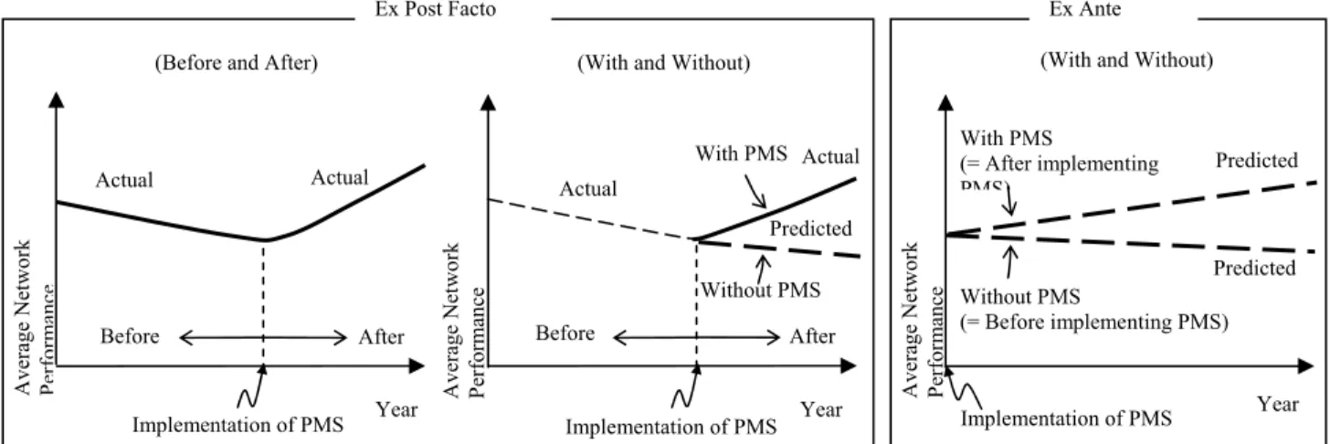
are going to implement PMS. Figure 1shows the concepts of the ex post facto and ex ante

evaluations. The ex post facto evaluation includes two types: a comparison of actual

performances, such as pavement condition, before and after PMS implementation (left hand side); and a comparison between predicted performance if PMS had not been implemented and actual performance after PMS implementation (center). Similar to the analyses of Hudson et al.

(15)

(2001), and Cowe Falls and Tighe (2004), the first type observes trends in pavement condition using time series data to compare differences before and after PMS implementation. The second type needs time series data of the actual pavement condition both before and after PMS

implementation as well. The actual pavement condition before PMS implementation is used to predict pavement condition without PMS after the year of PMS implementation based on a strategy used before PMS implementation (e.g., a worst first) and to compare this to the actual pavement condition with PMS after PMS implementation. This type includes the analysis by Smadi (2004). The improvement in the pavement conditions before and after PMS

implementation (left hand side) and with and without PMS implementation (center) represents the benefits of PMS implementation in terms of asset performance. Because the benefits accrue over years and are not shown immediately after PMS implementation, it is necessary to consider what an appropriate analysis period is in the analysis.

Since the time series data required for the ex post facto evaluation are rarely available in

transportation agencies, we need an alternative evaluation method. That is the ex ante evaluation

depicted in the right hand side in Figure 1. Using current performance data, two different future performances are predicted based on strategies: ‘without’ PMS implementation (e.g., a worst first strategy) and ‘with’ PMS implementation (i.e., a PMS optimization strategy). In addition,

since future pavement conditions can be simulated based on the strategies, the ex ante evaluation

can analyze the benefits of PMS implementation even if an agency had not implemented PMS. Although the predicted conditions do not represent real pavement condition, they can show the difference in pavement condition between ‘with’ and ‘without’ cases, that is, the benefits of PMS

implementation. As demonstrated, the ex ante evaluation is similar to the ex post facto evaluation

using a ‘with and without’ comparison in Figure 1 that compares predicted conditions without PMS implementation to actual conditions after PMS implementation. This is a quasi evaluation design recognizing the benefits of PMS between ‘with’ and ‘without’ cases.

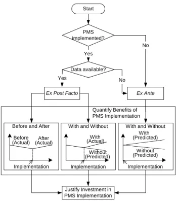
As described, the evaluation type is determined by analyzing whether PMS is already implemented and whether time series data are available before and after PMS implementation. Figure 2 depicts the flow diagram showing the process for quantifying the benefits of PMS implementation and justifying investment in PMS implementation.

Figure 1. Concepts of Ex Post Facto and Ex Ante Evaluations Year Implementation of PMS Average Net w ork Perfor m ance Before After Actual Actual

(Before and After)

Average Net w ork Perfor m ance Year Implementation of PMS Before After With PMS Without PMS Actual Actual Predicted (With and Without)

Ex Post Facto Ex Ante

Year Without PMS (= Before implementing PMS) With PMS (= After implementing PMS) Predicted Predicted Implementation of PMS (With and Without)

Average Net w ork Perfor m ance

(16)

Data available? Ex Ante Ex Post Facto No Yes Start Yes

Before and After With and Without With and Without

Before After

Implementation Implementation Implementation With (Predicted) Without (Predicted) PMS implemented? No Quantify Benefits of PMS Implementation Justify Investment in PMS Implementation Without (Actual) (Actual) (Actual) With (Predicted)

Figure 2. Flow Diagram

Benefit Quantification

Once we choose the evaluation design based on either the ex post facto evaluation or ex ante

evaluation, we compare performance ‘before’ and ‘after,’ or ‘with’ and ‘without’ PMS implementation. The comparison shows the differences in performance, which represent the benefits of PMS implementation. The benefits can be quantified by three analysis methods: a descriptive analysis based on common performance measures that capture improvements due to PMS implementation in terms of traffic and asset conditions; a regression analysis intended to quantify the contribution of PMS implementation to improved performance; and a benefit-cost analysis (BCA) to quantify monetary values of the benefits and costs of PMS and compare the benefits to the costs. The descriptive analysis and regression analysis can analyze various benefits of AMS implementation identified by Mizusawa and McNeil (2005) by using creative performance measures (e.g., degree of customer satisfaction in using improved assets), while BCA analyzes only benefits that can be monetized.

Descriptive Analysis

Recognizing the trends in an agency’s performance (e.g., pavement condition, budget, and expenditure), and exogenous effects (e.g., economy, traffic volume, and environment) in the context of an agency’s profile (types of assets, organizational structure, presence of legislation, and PMS) is an important first step. The descriptive analysis can show various trends using performance measures comparing before and after PMS implementation based on the ex post facto evaluation, or between with and without PMS implementation based on the ex ante evaluation.

One performance measure, the traffic weighted average pavement condition by year (Eq. (1)), can be used to capture one of the agency’s performance measures – pavement condition.

(17)

Also, this measure can illustrate users’ comfort in terms of riding quality, if pavement condition ratings focusing on surface characteristics, such as International Roughness Index (IRI) and Present Serviceability Rating (PSR) are used.

Traffic Weighted Average Pavement Condition =

∑

= = × × × n i i i n i i i i Length AADT Length AADT PCI 1 1 ) ( ) ( i = 1,…, n (1)

where PCI = pavement condition index in section i; AADT = annual average daily traffic in

section i; and Length = length of road sections in mile in section i. This measure can be plotted

by year. Differences between before and after conditions, or between with and without

conditions, can be illustrated visually. Summary statistics, for example, the average measurement value over a fixed analysis period can also be examined.

Regression Analysis

Using the network level performance measures developed for the descriptive analysis, regression analysis can be performed to address the weaknesses of the descriptive analysis, specifically, the inability to consider various changes simultaneously. This analysis is intended to observe the degree of independent variables’ influences on a dependent variable represented by the independent variables’ coefficients.

There are three components to the analysis: 1) Find an appropriate dependent variable representing the productivity of the investment in the PMS. We can assume productivity is an increase of PCI, increase of pavement life, reduction of M&R costs, and so on. It is necessary to explore various measures and determine an appropriate one. 2) Identify independent variables. 3) Determine a type of regression model. Among many types such as linear, polynomial, log linear, and so on, we should determine the best type by measure of fit (i.e., R-Square). We can also evaluate the statistical significance of the independent variables using t-values. An example of a

liner regression model using ‘with and without’ data based on the ex post facto and ex ante

evaluations is as follow:

Let TWAPCt be the traffic weighted average pavement condition in year t (Eq. (1)), Xtn be

the vectors of n independent variables (e.g., AADT, length, M&R treatment costs) in all road

sections in year t, and PMSt be the use of PMS in year t. The model to be estimated is:

t t t tn n t t t x x x PMS TWAPC =β₀ +β₁ ₁+β₂ ₂+...+β +δ +ε t = 1,…, T (2) where β0, β1,…, βn= coefficients; δt = a coefficient for the dummy variable, PMSt (i.e., δt is equal

to 1 if PMS is used in year t and equal to 0 otherwise); and ε t = error term associated with the

traffic weighted average pavement condition in year t. The dummy variable PMSt indicates the

impact of the use of PMS on the traffic weighted average pavement condition. If the coefficient of the variable is a positive value, PMS implementation improves the value of the traffic

weighted average pavement condition (i.e., benefits).

When ‘before and after’ data based on the ex post facto evaluation are used, the traffic

weighted average pavement conditions before and after PMS implementation do not align with the same analysis period. Hence, a linear regression without a dummy variable is used, and we can estimate the coefficients of the independent variables for ‘before’ and ‘after’ cases and compare them to each other. The differences in the comparison might be caused by PMS

(18)

determine the exact impact of PMS implementation on the traffic weighted average pavement condition as the dummy variable in Eq. (2) performs.

To build the models at the network level, time series data including pavement conditions and various measures, such as AADT, length, and M&R treatment costs, in all road sections are required. An ordinary least squares (OLS) regression is used to build the models, as the traffic weighted average pavement condition can be assumed to be independently and identically distributed.

Benefit-Cost Analysis

BCA is employed to show agency, user, and external benefits using monetary values. BCA uses alternatives for which benefits and costs can be measured in relative terms. Usually, each alternative addresses benefits produced by a project and costs incurred by the project. An important element of BCA is determining the perspective from which to conduct the analysis. As highway agencies provide a service, the analysis must be conducted from a social welfare

perspective, which recognizes the benefits to drivers. However, it is difficult to quantify the benefits of the service, because the drivers do not directly pay for the service as they do for a utility such as water. Hence, the benefits are most conveniently measured as incremental or relative benefits between a base case and ‘before’ case or ‘after’ case, or between a base case and ‘without’ case or ‘with’ case. A base case can be do-nothing (i.e., not adopting pavement

management). The base case and the cases with adoption of pavement management are assumed to be mutually exclusive.

The comparison of two alternatives, ‘before’ and ‘after’ cases, or ‘with’ and ‘without’ cases, can quantify the benefits of PMS implementation using the benefits derived from

pavement management compared to the base case and initial costs for M&R for each alternative. In order to compare two alternatives, we need to identify benefits and costs related to pavement management. As Hudson et al. (2001) and Cowe Falls and Tighe (2004) demonstrated, benefits and costs for before and after PMS implementation, or without and with PMS implementation,

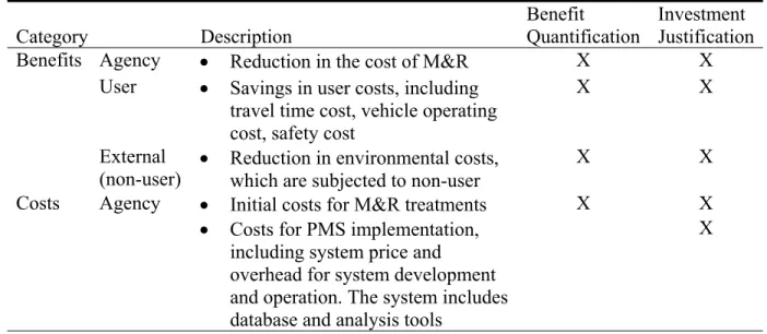
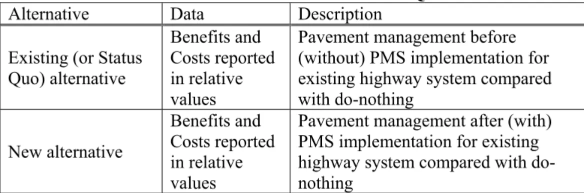
are required. Table 1 lists the benefits and costs related to pavement management used for

benefit quantification. Although there is a wide spectrum of qualitative benefits of PMS

implementation (Cowe Falls and Tighe 2004; Haas et al. 1994; Litzka et al. 2000; Smadi 2004; Sztraka 2001), we use the benefits that can be monetized.

The year-by-year benefits and costs (known as the cash flow) listed in Table 1 are estimated over the analysis period (Hendrickson and Wohl 1984). To estimate the benefits and costs for each alternative, we define:

• Bx,t = expected agency, user, and external benefits from alternative x during year t

(19)

Table 1. BENEFITS AND COSTS Category Description Benefit Quantification Investment Justification

Benefits Agency • Reduction in the cost of M&R X X

User • Savings in user costs, including

travel time cost, vehicle operating cost, safety cost

X X External

(non-user) • Reduction in environmental costs, which are subjected to non-user

X X

Costs Agency • Initial costs for M&R treatments X X

• Costs for PMS implementation,

including system price and overhead for system development and operation. The system includes database and analysis tools

X

The alternative x takes into account the ‘before’ and ‘after’ cases, or ‘without’ and ‘with’

cases, which already take into account incremental benefits derived from the comparison with the base case. Also, two other pieces of information must be specified:

• The analysis period, n: the mutually exclusive alternatives must be analyzed for the same and

concurrent analysis period to take into account the benefits and costs. The length of the analysis period depends on: 1) the expected life of an asset management project, and 2) the period in which we can fairly reliably predict benefits and costs (Hendrickson and Wohl 1984). It is necessary to decide the appropriate analysis period, since it is assumed that benefits and costs accrue over years.

• The discount rate, expressed in decimal form, i: although the benefits and costs arise from

different sources and are accrued or increased in different time periods throughout the

analysis period, we need to consider them at the same time in BCA. Since the monetary value changes over the analysis period, we have to set not only the specific time when we analyze the benefits and costs, but also the values of the benefits and costs to a consistent

(discounted) monetary value using a discount rate. In order to determine the discount rate, we can refer to the rate of return on money markets or the rate for all projects being considered by a decision-making unit such as the Office of Management and Budget (OMB) and the Congressional Budget Office (Weimer and Vining 2004).

To quantify the benefits of PMS implementation, either the Net Present Value (NPV) Method or the Benefit-Cost Ratio (BCR) Method can be used (Hendrickson and Wohl 1984). Here, we review the NPV Method.

First, the stream of benefits and costs are discounted to their present value and then netted to determine the net present value. For alternative ‘before’ and ‘after’ cases based on the ex post facto evaluation, the net present values for the n-year analysis period when the interest rate is the

(20)

Before: [NPVbeforePMS,n]i = [TPVBbeforePMS,n]i– [TPVCbeforePMS,n]i =

∑

= = = + − = + − + n t t t beforePMS t beforePMS n t t t beforePMS n t t t beforePMS i C B i C i B 0 , , 0 , 0 , ) 1 ( ) 1 ( ) 1 ( (3)

After: [NPVafterPMS,n]i = [TPVBafterPMS,n]i – [TPVCafterPMS,n]i =

∑

+ + = − + + + = − + + + = − + + − = + − + k n k n t t n k t afterPMS t afterPMS k n k n t t n k t afterPMS k n k n t t n k t afterPMS i C B i C i B 2 ) ( , , 2 ) ( , 2 ) ( , ) 1 ( ) 1 ( ) 1 ( (4)

where [TPVBx,α]i = total discounted benefits of alternative x for an α-year period and discount

rate i; [TPVCx,α]i = total discounted costs of alternative x for an α-year period and discount rate i;

and k = a period between ‘before’ and ‘after’ cases (k ≥ 1). The relationship between the three

analysis periods of ‘before k,’ ‘after k,’ and period k, is drawn in Figure 3. The analysis periods

of ‘before’ and ‘after’ begin at different years (i.e., the period of ‘after’ {t| n+k ≤ t ≤ 2n+k}

follows that of ‘before’ {t| 0 ≤ t ≤ n}). PMS is implemented in year n+k-1. As discussed in

Hudson et al. (2001), a longer period of k makes it easier to distinguish significant benefits between ‘before’ and ‘after’ cases. We note that other authors have used k=0, but this may lead to double counting.

Using Eq. (3) and (4), we calculate net present values for the alternatives and then compare them. That is, [NPVafterPMS,n]i – [NPVbeforePMS,n]i should be greater than zero. Since the before and after analysis does not use mutually exclusive alternatives as the

investments are sequential, this analysis is approximate.

For the ‘with’ and ‘without’ cases based on the ex post facto and ex ante evaluation, the net present value for the n-year analysis period with discount rate i ([NPVwithPMS,n]i and [NPVwithoutPMS,n]i) is:

Without: [NPVwithoutPMS,n]i = [TPVBwithtoutPMS,n]i – [TPVCwithoutPMS,n]i =

∑

= = = + − = + − + n t t t withoutPMS t withoutPMS n t t t S withtoutPM n t t t withoutPMS i C B i C i B 0 , , 0 , 0 , ) 1 ( ) 1 ( ) 1 ( (5)

With: [NPVwithPMS,n]i = [TPVBwithPMS,n]i – [TPVCwithPMS,n]i =

∑

= = = + − = + − + n t t t withPMS t withPMS n t t t withPMS n t t t withPMS i C B i C i B 0 , , 0 , 0 , ) 1 ( ) 1 ( ) 1 ( (6)

Uing Eq. (5) and (6), the difference in net present values [NPVwithPMS,n]i –

[NPVwithoutPMS,n]i is computed. Because the benefits and costs of ‘with’ and ‘without’ cases Figure 3. Relationship of Analysis Periods

n k n

0

Year t n n+k 2n+k

(21)

arise in the same time period, the analysis period, n, is considered. If the difference in the net present values either between ‘before’ and ‘after’ cases or between ‘with’ and ‘without’ cases is positive, PMS implementation is beneficial.

Investment Justification

Given the quantified agency, user, and external benefits of pavement management and costs for M&R treatments by BCA in the benefit quantification, it is possible to justify

investment in PMS implementation using BCA. BCA uses the incremental benefits of pavement management between ‘before’ and ‘after’ cases, or between ‘with’ and ‘without’ cases, and the costs for PMS implementation, and then directly analyzes whether investment in PMS

implementation is justifiable. The last column of Table 1 lists the benefits and costs related to

PMS implementation used for investment justification. This column differs from the column for the benefit quantification as the costs for PMS implementation are included.

Once the benefits and costs are specified, we need to conduct BCA using the NPV Method or the BCR Method. Again, we focus on the NPV method and extend Eq. (3) and (4)

using the incremental benefits derived from ‘before’ and ‘after’ cases based on the ex post facto

evaluation as follows:

[NPVPMS,n]i = {([TPVBafterPMS,n]i – [TPVCafterPMS,n]i) – ([TPVBbeforePMS,n] – [TPVCbeforePMS,n]i)} – [TPVCPMS,n]i =

∑

+ = = + + = − + + − ⎭ ⎬ ⎫ + − − ⎩ ⎨ ⎧ + − n k t t t PMS n t t t beforePMS t beforePMS k n k n t t n k t afterPMS t afterPMS i C i C B i C B 2 0 , 0 , , 2 ) ( , , ) 1 ( ) 1 ( ) 1 ( (7)

where [TPVCPMS,n]i = total discounted costs of PMS implementation for an n-year period and discount rate i. the last term recognizes that the PMS implementation costs may occur at any time during the analysis period but they must be discounted to be consistent with the ‘after’ benefits and costs. Since the analysis periods are different from each other, this ‘before and after’ comparison violates the rule of consistent analysis periods. Hence, this comparison uses

approximate benefits and costs to justify investment similar to that conducted by Cowe Falls and Tighe (2004).

Using the incremental benefits derived from ‘with’ and ‘without’ cases based on the ex

post facto and ex ante evaluations, the net present value for the n-year analysis period with discount rate i is:

[NPVPMS,n]i = {([TPVBwithPMS,n]i – [TPVCwithPMS,n]i) – ([TPVBwithoutPMS,n]i – [TPVCwithoutPMS,n]i} – [TPVCPMS,n]i =

∑

= = = + − ⎩ ⎨ ⎧ ⎭ ⎬ ⎫ + − − + − n t t t PMS n t n t t t withoutPMS t withoutPMS t t withPMS t withPMS i C i C B i C B 0 , 0 0 , , , , ) 1 ( ) 1 ( ) 1 ( (8)

Because the benefits of ‘with’ and ‘without’ cases and the costs of PMS implementation arise from the same time, only the analysis period, n, is considered. If the net present value of Eq. (7) or (8) (i.e., the monetized benefits of pavement management between ‘after’ and ‘before’ cases, or between ‘with and ‘without’ cases, minus the costs for PMS implementation) is

(22)

Efficacy, Effectiveness and Efficiency: The 3Es

Drawing on work in Soft Systems Methodology (Checkland 1999), we distinguish among different approaches to quantifying the benefits of PMS implementation and justifying

investment in PMS implementation, with respect to the 3Es (that is, efficacy, effectiveness, and efficiency) defined as follows:

• Efficacy: shows whether PMS work or not. The efficacy can be recognized by the difference

in performance between ‘before’ and ‘after,’ or between ‘with’ and ‘without,’ using

descriptive analysis and regression analysis. Also, the BCA quantifies the efficacy using the net benefits (i.e., benefits including reductions in agency, user, and external costs minus M&R costs), and the ratio of benefits to costs for M&R treatments.

• Effectiveness: identifies the degree to which PMS achieve the agency’s asset management

goals. Effectiveness is determined by the difference, but needs to be addressed in term of degree. If the degree is addressed, an agency can observe to what extent asset conditions meet their asset management goals compared to the case of ‘before’ or ‘without.’ The results of descriptive analysis, regression analysis, and BCA can articulate the effectiveness.

• Efficiency: identifies optimal use of resources using the ratio of output or outcome to input of

PMS. Efficiency can be quantified by the comparison of the ratios of benefits to costs for M&R treatments between ‘before’ and ‘after,’ or between ‘with’ and ‘without.’ If the costs for M&R before and after, or with and without PMS implementation are available, the different ratios of performance (e.g., pavement condition) to the costs between ‘before’ and ‘after,’ or between ‘with’ and ‘without,’ assess the efficiency of PMS implementation. All three analysis methods are capable of assessing the efficiency.

Three Analysis Methods

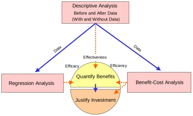
The generic methodology embraces the three analysis methods addressed above to obtain richer insight into PMS implementation as shown in Figure 4. The descriptive analysis identifies data consisting of various performance measures. The differences in the performance measures between ‘before’ and ‘after’ cases, or between ‘with’ and ‘without’ cases, show the benefits of PMS implementation in terms of the 3Es as well as various trends of the agency’s performance and exogenous effects. Then the data are entered into the regression analysis and BCA to quantify the benefits of PMS implementation in terms of monetary values, as well as the

performance measures. Since the regression analysis and BCA utilize ‘before and after,’ or ‘with and without’ data, they are under the umbrella of the descriptive analysis. These analyses also quantify the benefits in terms of the 3Es. Afterwards, the quantified benefits are used for justifying investment in PMS implementation with BCA in terms of efficiency. Since there are pros and cons in each analysis method (Mizusawa and McNeil 2005), it is necessary to take into account how these methods are used, together or independently. The following case study provides an illustration of the mechanism and nuances of manipulating the data to be able to support the analysis.

(23)

4. Case Study

A case study was conducted to apply the generic methodology and evaluate the implementation of Highway Economic Requirement System - State Version (HERS-ST) in terms of benefit quantification and investment justification with respect to the 3Es. HERS-ST, created by the Federal Highway Administration (FHWA), is a highway investment/performance computer model, which determines the impact of alternative highway investment levels and program structures (e.g., widening, resurfacing, and reconstruction) on highway conditions, performance, and agency, user, and external costs. HERS-ST uses data from the Highway Performance Monitoring System (HPMS). HPMS is a national level highway information system, including data related to the extent, conditions, performance, use and operating characteristics of highways (FHWA 2002). This case study uses 2001 HPMS data from the state of New Mexico included in the HERS-ST package (which is downloadable via the FHWA’s website). Because the data captures highway inventory and performance in year 2001 only, the comparison of ‘with’ and

‘without’ cases based on the ex ante evaluation is conducted. A 10-year analysis period from

2001 to 2010 was set.

The highway network included in the HPMS data has 283 sections consisting of rural principal arterials, rural minor arterials, and urban principal arterials. Rural principal arterials are the largest class (66.7% in lane-miles). Rural minor arterials are the second largest functional class (19.9% in lane-miles). Urban principal arterials are smallest among the three classes (13.4 % in lane-miles). The largest portion of the network falls into fair, good, and very good

pavement conditions (98.8% in lane-miles) in terms of PSR, which is a subjective pavement rating system based on a scale of 1 to 5.

Using the data, two different scenarios are simulated, a HERS-ST strategy (i.e., ‘with’ case) and a worst first strategy (i.e., ‘without’ case). It is presumed that the difference between the two scenarios shows the benefits of HERS-ST implementation in pavement condition. The condition without HERS-ST may simulate the condition before HERS-ST implementation, while the condition with HERS-ST may simulate the condition after HERS-ST implementation.

The two strategies, worst first strategy and HERS-ST strategy, are used by HERS-ST per se to estimate future performances in the ‘without’ case and the ‘with’ case, respectively. The worst first strategy focuses only on sections that have deficiencies with respect to deficiency

Figure 4. Relationship of Analysis Methodology Efficiency Effectiveness Efficiency Efficacy Benefit Quantification Investment Justification Benefit-Cost Analysis Regression Analysis Descriptive Analysis (before and after data or

with and without data)

Data Flow Analysis Flow

(24)

criteria used by HERS-ST and assigns treatments (i.e., do-nothing, resurfacing, and

reconstruction) based on the criteria. For example, a section with worse condition and higher AADT is prioritized for treatments. Meanwhile, the HERS-ST strategy assigns the most appropriate treatment that has a highest benefit-cost ratio among potential treatments (i.e., do-nothing, resurfacing, resurfacing with shoulder improvements, resurfacing high-cost lanes, and reconstruction) for each highway section (FHWA 2006).

The ‘without’ case is developed by overriding treatment recommendations produced by HERS-ST with user-specified treatments that are included in State Improvements data. By making State Improvement data override HERS-ST recommended treatments, a user can analyze the impacts of user-specified treatments compared with those of HERS-ST recommended

treatments, with respect to various performance measures. The HERS-ST recommended treatments represents the ‘with’ case.

5. Results

Following the analysis methods described in the previous section, the benefits of using HERS-ST are assessed using aggregate data as follows:

Benefit Quantification

Using the three analysis methods, the benefits of HERS-ST implementation are quantified in terms of the 3Es as follows:

Descriptive Analysis

HERS-ST runs its analysis for ‘with’ and ‘without’ cases while adjusting the ‘without’ case so that initial investments in improvements are equal to the ‘with’ case, since the difference in the initial costs between ‘with’ and ‘without’ cases was recognized.

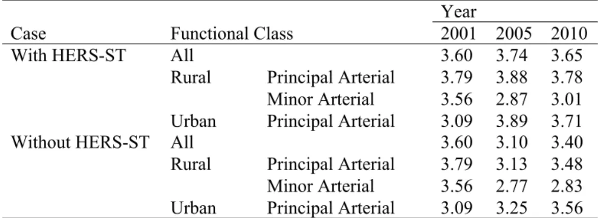
Table 2 shows the traffic weighted average pavement condition from 2001 to 2010 for ‘with’ and ‘without’ cases. For all road functional classes, the mean with HERS-ST is 0.30 points (=3.67-3.37) higher than that without HERS-ST. The increase is equivalent to 9 % (=0.30/3.37) of the traffic weighted average pavement condition without HERS-ST. Among the three functional classes, rural principal arterials show the highest point increase at 0.35 (=3.82-3.46), while rural minor arterials show the lowest point increase at 0.09 (=3.15-3.05). Hence, HERS-ST maintains stable and good pavement conditions of all functional classes over 10 years.

Table 2. COMPARISON OF TWAPC

Case Functional Class

Year

2001 2005 2010

With HERS-ST All 3.60 3.74 3.65

Rural Principal Arterial 3.79 3.88 3.78

Minor Arterial 3.56 2.87 3.01

Urban Principal Arterial 3.09 3.89 3.71

Without HERS-ST All 3.60 3.10 3.40

Rural Principal Arterial 3.79 3.13 3.48

Minor Arterial 3.56 2.77 2.83

(25)

The descriptive analysis showed the differences between various performance measures, including the traffic weighted average pavement condition, provided by HERS-ST between the ‘with’ and ‘without’ cases. The differences demonstrate the efficacy – whether HERS-ST works or not, and the effectiveness – how much HERS-ST improves performance such as pavement condition.

Regression Analysis

Regression analysis employed the traffic weighted average pavement condition to capture the benefits of HERS-ST implementation in the network level based on Eq. (2) as follows:

Let TWAPSRn be the traffic weighted average PSR in funding period n, AADTn be the total

annual average daily traffic in all sections in funding period n, and HERSn be the use of

HERS-ST in funding period n. The model to be estimated is:

n n n n n AADT HERS TWAPSR =β₀ +β₁ +δ₁ +ε (9)

where β0 and β1 = coefficients; δn = coefficient for dummy variable (e.g., δn is equal to 1 if

HERS-ST is used in funding period n and equal to 0 otherwise); and ε n = error term associated

with the nth_{traffic weighted average PSR. Since there are only six observations (i.e., 3 specific}

years×2 cases), however, the result is not meaningful from a statistical perspective. If there are

enough observations, the coefficient for the dummy variable shows the efficacy and effectiveness of PMS implementation.

Benefit-Cost Analysis

Given the output results of HERS-ST, we found that the ‘with’ case is more efficient in keeping good pavement conditions in the network level, because the ‘with’ case can obtain higher benefits, including agency, user, and external benefits, using almost the same total initial cost as the ‘without’ case. For example, BCR of the ‘with’ case is 7.860, while that of the ‘without” case is 5.282, for all road functional classes over 10 years. Also, the results

demonstrate that HERS-ST implementation produces net benefits of $2.0 billion (based on 2004 dollars) over BCA period, because there are differences in the total benefits between ‘with’ and ‘without’ cases. The BCA period corresponds to the duration of treatments’ lives. For example, a simple resurfacing takes one or two funding periods (i.e., 5 to 10 years) as a BCA period. In case of significant treatments, the BCA period can extend beyond the end of the overall analysis period (i.e., 20 years in this case study) (FHWA 2005).

Also, the results imply that HERS-ST implementation results in total net benefits, at least $359 million, over 10 years. This amount does not include the benefits from 2006 to 2010 derived from M&R treatments applied between 2001 and 2005. The benefits consist of $1.5 million agency benefits, $323 million user benefits, and $34.5 million external benefits. These values are based on 2004 dollars. These results demonstrate the efficacy and effectiveness of HERS-ST implementation in terms of monetary values and the efficiency in terms of BCR.

Investment Justification

Given the quantified total discounted benefits of HERS-ST implementation, we can compare the benefits to ST implementation costs in order to justify investment in HERS-ST implementation. Since there are no available data related to implementation costs, this

(26)

discussion of whether the benefits exceed HERS-ST implementation costs remains academic. However, using the quantified total benefits, from the point of view of net social welfare, the following statements can be made:

• If an agency spends less than $359 million on implementation over 10 years, the agency can

justify the investment in HERS-ST implementation, or

• If an agency spends less than $2.0 billion on implementation over 25 years, the agency can

justify the investment in HERS-ST implementation.

From the agency perspective, if the agency spends less that $1.5 million on

implementation over 10 years, the agency can justify the investment in HER-ST implementation. Although these net benefit estimates are underestimated, it is not expected that HERS-ST

implementation costs would approach $359 million, or even $1.5 million over 10 years, because HERS-ST is a free application distributed by FHWA.

6. Discussion

The results of the case study showed the benefits in pavement conditions between ‘with’ and ‘without’ cases. These benefits are due to the fact that different treatments were applied to 46% of the sections in the ‘with’ case compared to the ‘without’ case over 10 years.

In the ‘with’ case, the preventive treatments are applied to about 30% of treatments (i.e., same treatments: 12%, and different treatments: 18%). Figure 5 depicts the decision-making concepts used to determine treatments in the ‘with’ and ‘without’ cases with respect to pavement deterioration curves. The horizontal line in the graph shows the treatment threshold between resurfacing and reconstruction in terms of PSR. The ‘with’ case determines the timing of treatments based on the predicted pavement conditions at the end of a current funding period (FHWA 2005). For example, since the ‘with’ case can observe the deterioration curve goes

below the threshold at year t during the five years’ funding period based on the predicted

pavement condition, the resurfacing that is less expensive than reconstruction is recommended to

be conducted at year t. Meanwhile, the ‘without’ case focuses on the initial pavement conditions

of the current funding period and thus assumes that resurfacing is not required. Because of the loss of a timely treatment, the pavement condition will degrade continuously. Hence, the

‘without’ case needs to employ a more aggressive treatment than the ‘with’ case in order to keep the pavement in good condition; the aggressive treatment overextends the budget for M&R; and the ‘without’ case loses benefits that are accrued in the ‘with’ case.

Figure 5. Conceptual Decision-Makings between ‘With’ and ‘Without’ Cases With Without 0 PSR Year 5 Resurfacing Reconstruction t

(27)

The ‘with’ case considers four types treatment types, while the ‘without’ case considers two treatment types. These different treatment types applied between resurfacing and

reconstruction accrues benefits as well. The ‘without’ case has 60 sections or 180 lane-miles of reconstruction, while the ‘with’ case has 16 sections or 17 lane-miles. On the other hand, the ‘with’ case has 104 sections or 617 lane-miles of resurfacing with shoulder improvement, while the ‘without’ case has 15 sections or 122 lane-miles (these are automatically assigned by HERS-ST, although the ‘without’ case does not consider the treatment). It is assumed that the ‘with’ case considers the resurfacing with shoulder improvement as an appropriate treatment type, but not the reconstruction used in the ‘without’ case. Since the unit cost of resurfacing with shoulder improvement is less expensive than that of reconstruction (e.g., 60-70% less expensive in urban principal), the ‘with’ case can treat much more pavements than the ‘without’ case (1.12 times in number of sections; 1.19 times in lane-miles). The ‘with’ case uses less expensive treatments than the ‘without’ case, and allows investment in further treatments.

The generic methodology includes three analysis methods: descriptive analysis,

regression analysis, and BCA. Since the generic methodology is associated with various data, it is necessary to take into account the following data issues. Concerning the descriptive analysis and regression analysis, these methods require several performance measures associated with a

particular asset. To conduct an ex post facto evaluation using ‘before and after’ data (i.e., time

series data), the data need to include the performance measures used in the descriptive analysis

and regression analysis. To conduct an ex post facto evaluation and ex ante evaluation using

‘with and without’ data, we need to predict future performances based on past or current performance with respect to the performance measures used in the analyses. To obtain the predicted performance measures, simulations based on various models (e.g., a deterioration model, speed model, and travel forecast model in HERS-ST) are required, while taking into

account data related to infrastructure, traffic, and treatments and consequences. Hence, the ex

ante evaluation needs additional data to simulate predicted performance as well as performance

measures used in the descriptive analysis and regression analysis. The third analysis method,

BCA, estimates agency, user, and external benefits. Hence, in both the ex post facto and ex ante

evaluations, BCA requires data related to cost valuation.

This case study based on the ex ante evaluation addressed the positive results in the benefit

quantification and the investment justification. In case of using the ex post facto evaluation, a

result may not show benefits because of external influences (e.g., economy, environment, etc.) rather than HERS-ST implementation and the degree of conformity of an agency’s business to the M&R program recommended by HERS-ST.

The outcomes of this case study showed the HERS-ST’s ability to predict future pavement conditions, quantify detailed benefits based on elaborate functions derived from numerous past studies, and possibly justify investment in HERS-ST implementation compared to the costs for

implementation. This implies that AMS which posses the required various data and simulation

models to estimate assets conditions and benefits can analyze their benefits and investment using the generic methodology. Since collecting required data and developing simulation models are time consuming and complex tasks, the use of AMS to simulate predicted conditions and quantify benefits is recommended. Needless to say, it is important to determine appropriate simulation and valuation methods while focusing on specific assets. Also, in the case of

(28)

necessary to have common performance measures in the descriptive analysis, the regression analysis, and the BCA.

7. Conclusions

A generic methodology for quantifying the benefits of AMS implementation and justifying investment in AMS implementation is presented in this paper. The generic

methodology involves three analysis methods: descriptive analysis, regression analysis, and BCA. These methods rely on two evaluations: an ex post facto evaluation and an ex ante

evaluation depending on the implementation of AMS and the availability of time series data. The case study analyzed the benefits of HERS-ST by focusing on pavement used an ex ante

evaluation. The results showed the applicability of the generic methodology to quantify the benefits of HERS-ST implementation with respect to the 3Es. Also, the results identified the improvements in pavement conditions and the benefits of HERS-ST implementation consisting of agency, user, and external benefits. The case study suggested that HERS-ST implementation contributes to an improvement in agencies’ performance and costs for M&R, and that the benefits derived from HERS-ST implementation will exceed costs for implementation and operation. Although the generic methodology is applied to HERS-ST only, the approach is rational and grounded in widely accepted practices for any AMS evaluation. The methodology and case study underscored some of the data challenges as data is not necessarily modeled or collected specifically for this type of analysis. The use of the generic methodology may reinforce the implementation and development of AMS through the articulation of benefits and

justification of investment in transportation agencies. Executive Summary References

Cambridge Systematics, I., PB Consult, System Metrics Group, Inc. (2005). "Analytical Tools

for Asset Management." National Cooperative Highway Research Program Report 545,

Transportation Research Board, Washington, D.C.

Checkland, P. (1999). Systems Thinking, Systems Practice, John Wiley & Sons, Chichester, West

Sussex, England; New York.

Cowe Falls, L., and Tighe, S. (2004). "Analyzing Longitudinal Data to Demonstrate the Costs

and Benefits of Pavement Management." Journal of Public Works Management and Policy,

8(3), 176-191.

Federal Highway Administration (FHWA). (2006). Highway Economic Requirements System -

State Version. User's Guide, Software Version 4.X.

Federal Highway Administration (FHWA). (2005). Highway Economic Requirement System -

State Version. Technical Report.

Federal Highway Administration (FHWA). (2002). "About highway performance monitoring system (HPMS)." <http://www.fhwa.dot.gov/policy/ohpi/hpms/abouthpms.htm> (Nov. 26, 2006).

Flintsch, G. W., Dymond, R., Collura, J. (2004). "Pavement Management Applications using

Geographic Information Systems." National Cooperative Highway Research Program

Synthesis of Highway Practice 335,Transportation Research Board, Washington, D.C.

Haas, R., Hudson, W. R., Zaniewski, J. (1994). Modern Pavement Management, Krieger

(29)

Hudson, W. R., Hudson, S. W., Visser, W., and Anderson, V. (2001). "Measurable Benefits

Obtained from Pavement Management." Proc., 5th International Conference on Managing

Pavements, Seattle, Washington.

Litzka, J., Scazziga, I., Woltereck, G. (2000). "Experiences with Implementation of Similar PMS

in Austria, Germany and Switzerland." Proc., 1st European Pavement Management Systems

Conference, Budapest, Hungary.

Mizusawa, D., and McNeil, S. (2006). "Synthesizing Experiences of Implementing Asset Management in the World: Lessons Learned from Pavement Management Case Studies."

Transport Policy Studies' Review, 9(34), 21-30.

Mizusawa, D., and McNeil, S. (2005). "Quantify the Benefits of Implementing Asset

Management." Proc., 1st Annual Inter-University Symposium on Infrastructure Management,

Waterloo, Canada.

Smadi, O. (2004). "Quantifying the Benefits of Pavement Management." Proc., 6th International

Conference on Managing Pavements, Queensland, Australia.

Sztraka, J. K. (2001). "Quantifiable Benefits of Pavement Management in Aid of Setting and

Achieving Goals." Proc., 5Th International Conference on Managing Pavements, Seattle,

Washington.

Weimer, D. L., and Vining, A. R. (2004). Policy Analysis: Concepts and Practice, 4th Ed.,

Pearson Prentice Hall, .

Wohl, M., and Hendrickson, C. (1984). Transportation Investment and Pricing Principles: An

(30)

PART I: INTRODUCTION TO ASSET MANAGEMENT

Part I of this report presents the research problem addressed and the research goals and objectives. This section begins by raising the problems to be addressed and presenting the background and context for this research. The next chapter introduces the goals and objectives, approach, scope, and includes an outline of the remainder of the report.

(31)

Chapter 1. The Problem

Transportation agencies have identified asset management (AM) as a concept to support cost effective maintenance and rehabilitation decisions related to physical assets. Asset

Management Systems (AMS) and tools are required to implement these AM concepts.

For transportation agencies, it is expected that AM improves agencies’ performance in terms of the performance of their assets while it reduces agencies’ cost for maintenance and rehabilitation (M&R). In a worst case scenario without asset management, M&R costs would continue to increase over time because of infrastructure deterioration caused by increases in the vehicle miles of travel, the increase in heavy trucks, aging infrastructure, and inappropriate M&R strategies. At the same time, the performance would degrade because M&R cannot catch up with the pace of deterioration of infrastructure due to the aforementioned reasons and an agency cannot afford to invest in the additional M&R needed due to budget constraints. Ultimately, the degradation in performance will translate to increased user costs. After implementing an AMS, appropriate M&R identified using the decision support tools in the AMS may improve

performance and reduce costs simultaneously. Also, it is noted that there would be a reduction in user and external costs because appropriately maintained roads provide a better driving

environment for users, thus reducing operational costs, crash costs, travel time costs, and environmental impacts.

Agencies are often hesitant to move forward in implementing AMS and tools, because it is difficult to document whether the benefits produced by AMS or tools exceed the costs for implementation and operation. Indeed six of seven research needs studies conducted since 2000 have identified “Measuring Benefits” as an important area of research to develop the base of support for asset management (Switzer and McNeil, 2004).

Understanding the relationship between the improvement of agencies’ performance and costs for M&R is challenging. A new method is required to measure the benefits of

implementing AMS and to demonstrate whether the benefits exceed the AMS implementation and operation costs. The method must be generic and adapt to different AMS and tools and applied to a variety of agencies with different resources.

The goal of the research is to develop a generic methodology for measuring the benefits derived from implementing an AMS. Benefits are defined as improvements in the transportation agency’s business performance as well a