Currency Hedging Strategies Using Dynamic Multivariate GARCH

(1)

Currency Hedging Strategies Using Dynamic Multivariate

GARCH

Lydia González-Serrano

Department of Business Administration Rey Juan Carlos University

Juan-Angel Jimenez-Martin

Department of Quantitative Economics Complutense University of Madrid

October 2011

* The authors are most grateful for the helpful comments and suggestions of participants at the International Conference on Risk Modelling and Management, Madrid, Spain, June 2011, especially to M. McAleer and T. Pérez Amaral. The second author acknowledges the financial support of the Ministerio de Ciencia y Tecnología and Comunidad de Madrid, Spain.

(2)

Abstract

This paper examines the effect on the effectiveness of using futures contracts as hedging instruments of: 1) the model of volatility used to estimate conditional variances and covariances, 2) the analyzed currency, and 3) the maturity of the futures contract being used. For this purpose, daily data of futures and spot exchange rates of three currencies, Euro, British pound and Japanese yen, against the American dollar are used to analyze hedge ratios and hedging effectiveness resulting from using two different maturity currency contracts, near-month and next-to-near-month contract. Following Tansuchat, Chang and McAleer (2010), we estimate four multivariate volatility models (CCC, VARMA-AGARCH, DCC and BEKK) and calculate optimal portfolio weights and optimal hedge ratios to identify appropriate currency hedging strategies. Hedging effectiveness index suggests that the best results in terms of reducing the variance of the portfolio are for the USD/GBP exchange rate. The results show that futures hedging strategies are slightly more effective when the near-month future contract is used for the USD/GBP and USD/JPY currencies. Moreover, CCC and AGARCH models provide similar hedging effectiveness although some differences appear when the DCC and BEKK models are used.

Keywords: Multivariate GARCH, conditional correlations, exchange rates, optimal

hedge ratio, optimal portfolio weights, hedging strategies.

(3)

1. Introduction

With the rise of the capital market liberalization and globalization, foreign currency denominated assets circulate rapidly in the world. With increasing internationalization of financial transactions, the foreign exchange market has been profoundly transformed and became more competitive and volatile. This places the accurate and reliable measurement of market risks in a crucial position for both investment decision and hedging strategy designs.

Foreign exchange rate markets are the largest and most liquid of all asset markets. Developments in these markets influence national trade and monetary policies and the competitiveness of nations. Foreign exchange markets are also important for the increasing number of companies engaged in cross-border trade and investment. The foreign exchange business is naturally risky, because it deals primarily in measuring, pricing, and managing risk. The success of an institution trading in the foreign exchange market depends critically on how well it assesses prices and manages the inherent risk, on its ability to limit losses from particular transactions, and to keep its overall exposure under control.

The fact in managing currency risk is to control the volatility of the portfolio. The volatility of a portfolio includes variances and correlation coefficients of, and among, individual positions. Great losses may be yielded from holding this portfolio without a time-varying consideration of its variance and correlation parts simultaneously. If investors can sense the interacting dynamics among markets in advance, then adjusting and hedging activities will be implemented in time. Successful and profitable performances can therefore be made.

The aim of hedging is to use derivatives to reduce a particular risk. A relatively inexpensive and reliable strategy for hedging foreign exchange risk involves the use of foreign currency futures markets. Hedging with futures contracts is perhaps the simplest method for managing market risk arising from adverse movements in the foreign exchange market. Hedgers usually short an amount of futures contracts if they hold the long position of the underlying currency and vice versa. The question is how many

(4)

effectiveness measure of that ratio. The hedge ratio provides information on how many futures contracts should be held, whereas its effectiveness evaluates the hedging performance and the usefulness of the strategy. In addition, hedgers may use the effectiveness measure to compare the benefits of hedging a given position from many alternative contracts.

Generally speaking, when the market trend is stable, the hedge ratio will become smaller, whereas if a big fluctuation of the market takes place it will get bigger. Several distinct approaches have been developed to estimate the optimal hedge ratio (OHR), also known as the minimum-variance hedge ratio.

The static hedging model with futures contracts (Johnson [32], Stein [56], Ederington, [21]) assumes that the joint distribution of spot and futures returns is time-invariant and therefore the OHR, defined as the optimal number of futures holdings per unit of spot holdings, is constant over time. The minimum variance OHR use to be derived form the ordinary-least squares (OLS) regression of spot price changes on future price changes. There is wide evidence that the simple OLS method is inappropriate to estimate hedge ratios since it suffers from the problem of serial correlation in the OLS residuals and the heteroscedasticity often encountered in spot and futures price series (Herbst et al. [31]).

Therefore, the underlying assumption of the static hedging model of time-invariant asset distributions has been changed. The Autoregressive Conditional Heteroscedastic (ARCH) framework of Engle [23] and its extension to a generalized ARCH (GARCH) structure by Bollerslev [8] have proven to be very successful in modelling asset price second-moment movements. Bollerslev [9], Bailie and Bollerslev [3], and Diebold [19] have shown that the GARCH (1,1) model is effective in explaining the distribution of exchange rate changes. However, Lien et al. [39] compared Ordinary Least Squares (OLS) and constant-correlation vector generalized autoregressive conditional heteroscedasticity (VGARCH) and claimed that the Ordinary List Squares (OLS) hedge ratio performs better than the VGARCH one. CHAN [16] proposed a dynamic hedging strategy based on a bivariate GARCH-jump model augmented with autoregressive jump intensity to manage currency risk. The collective evidence shows that the GARCH-modelled dynamic hedging strategies are empirically appropriate but the risk-reduction

(5)

improvements over constant hedges vary across markets and may be sensitive to the sample period employed in the analysis.

Regarding foreign currencies, different results are provided. Kroner and Sultan [35] demonstrated that GARCH hedge ratios produce better hedging effectiveness than conventional hedge ratios in currency markets. Chakraborty and Barkoulas [15] employed a bivariate GARCH model to estimate the joint distribution of spot and futures currency returns and they constructed the sequence of dynamic (time-varying) OHRs based upon the estimated parameters of the conditional covariance matrix. The empirical evidence strongly supports time-varying OHRs but the dynamic model provides superior out-of-sample hedging performance, compared to the static model, only for the Canadian dollar. Ku et al. [37] applied the dynamic conditional correlation (DCC)-GARCH model of Engle [24] with error correction terms to investigate the optimal hedge ratios of British and Japanese currency futures markets and compare the DCC-GARCH and OLS model. Results show that the dynamic conditional correlation model yields the best hedging performance.

Given the distinct theoretical advantages of the dynamic hedging method over the static one, a great number of studies have employed the multivariate GARCH framework to examine its hedging performance for various assets. To evaluate the impact of model specification on the forecast of conditional correlations, Hakim and McAleer [29] analyze whether multivariate GARCH models incorporating volatility spillovers and asymmetric effect of negative and positive shocks on the conditional variance provide different conditional correlations forecasts. Using three multivariate GARCH models, namely the CCC model (Bollerslev, [10]), VARMA-GARCH model (Ling and McAleer, [41]), and VARMA-AGARCH model (McAleer et.al., [45]) they forecast conditional correlations between three classes of international financial assets (stock, bond and foreign exchange rates). The paper suggested that incorporating volatility spillovers and asymmetric of negative and positive shocks on the conditional variance does not affect forecasting conditional correlations.

To estimate time-varying hedge ratios using multivariate conditional volatility models Chang et.al. [17] examinned the performance of four models (CCC, VARMA-GARCH,

(6)

crude oil markets (BRENT and WTI). The calculated OHRs form each multivariate conditional volatility model presented the time-varying hedge ratios and recommended to short in crude oil futures, with a high portion of one dollar long in crude oil spot. The hedging effectiveness indicated that DCC (BEKK) was the best (worst) model for OHR calculation in terms of the variance of portfolio reduction.

This paper extends Chang et.al. [17] to currency hedging. To evaluate the impact of model specification on conditional correlations forecasts, this paper calculates and compares the correlations between conditional correlations forecasts resulted from four different multivariate models (CCC, VARMA-AGARCH, DCC and BEKK) to estimate the returns on spot and futures (analyzing two sets of futures depending on their maturity) of three currency prices (USD/GBP, USD/EUR and USD/JPY). The purpose is to calculate the optimal portfolio weights and OHRs ratio from the conditional covariance matrices in order to achieve an optimal portfolio design and hedging strategy, and to compare the performance of OHRs from estimated multivariate conditional volatility models by applying the hedging effectiveness index. One of the main contributions of this study is that allows us to compare whether the results are different depending on the volatility model, currency and maturity of the futures contract selected. We have found no evidence of these three items considered together for currency hedging in prior literature.

The remainder of the paper is organized as follows. In Section 2 we discuss the multivariate GARCH models used, and the derivation of the OHR and hedging effective index. In section 3 the data used for estimation and forecasting and the descriptive statistics are presented. Section 4 analyses the empirical estimates from empirical modeling. Section 5 presents some conclusions.

2. Econometric Models

2.1. Multivariate Conditional Volatility Models

Following Chang et.al. [17] this paper considers the CCC model of Bollerslev [10], VARMA-AGARCH model of McAleer et al. [45], the DCC model of Engle [24] and

(7)

in the first two models while dynamic conditional correlations are taken in the last two models.

Considering the CCC multivariate GARCH model of Bollerslev [10]:





1 t/ t 1 t, t t t y E y F_   D (1)



1



var _t/F_t_  D D_t _t

Where y_t 



y₁_t,...,y_mt



, _t 



₁_t,...,_mt



 is a sequence of independent and identically distributed random vectors, Ft is the past information available at time t,



1/ 2 1/ 2



1 ,...,

t m

D diag h h , m is the number of assets (see, for example, McAleer [43] and Bauwens et al. [6]). As  E



 _{t t}/F_t_₁



E



 _t 



, where  

 

_ij for i, j = 1,…,

m, the constant conditional correlation matrix of the unconditional shocks, _t , is equivalent to the constant conditional covariance matrix of the conditional shocks, ,_t from (1),  _{t t}D_{t t t} D D_t, _t 



diagQ_t



1/2,and E



 _{t t}/F_t_₁



Q_t  D D_t _t,where Q_t is the conditional covariance matrix.

The CCC model of Bollerslev [10] assumes that the conditional variance for each return,h_it, i =1, …, m, follows a univariate GARCH process, that is

2 , , 1 1 , r s it i ij i t j ij i t j j j h    _  h _    







(2)

where _ij represents the ARCH effect, or short run persistence of shocks to return i, _ij represents the GARCH effect, and

1 1 r s ij ij j j     



denotes the long run persistence. The CCC model assumes that negative and positive shocks of equal magnitude have identical impacts on the conditional variance. McAleer et al. [45] extended the

(8)

on the conditional variance, and proposed the VARMA-AGARCH specification of the conditional variance as follows:

, 1 1 1 r r s t i t i i t i t i j t j i i j H W A_ C I __ B H _     



 



 



(3)

Where Ci are mm matrices for i = 1,…r with typical element _ij, and



1,...,



,

t t mt

I diag I I is an indictor function, given as

 

0, 0 1, 0 it it it I         _    (4)

If m=1 (3) collapses to the asymmetric GARCH (or GJR) model of Glosten et al. [28]. If Ci = 0 and Ai and Bj are diagonal matrices for all i and j, then VARMA-AGARCH reduces to the CCC model. The structural and statistical properties of the model, including necessary and sufficient conditions for stationarity and ergodicity of VARMA-AGARCH, are explained in detail in McAleer et al. [45]. The parameters of model (1) to (3) are obtained by maximum likelihood estimation (MLE) using joint normal. We also estimate the models using Student’s t distribution, in this case the appropriate estimator is QMLE.

The assumption that the conditional correlations are constant may seen unrealistic so, in order to make the conditional correlation matrix time dependent, Engle [24] proposed a dynamic conditional correlation (DCC) model, which is defined as

1 (0, ), 1, 2,..., t t t y _  Q t n (5) , t t t t Q  D D (6) where



1/ 2 1/ 2



1 ,..., t m

D diag h h is a diagonal matrix of conditional variances, and _t is the information set available at time t. The conditional variance, hit, can be defined as a univariate GARCH model, as follows:

(9)

, , 1 1 p q it ik i t k il i t l k l h    _  h _    







(7)

If _tis a vector of i.i.d. random variables, with zero mean and unit variance, Qt in (8) is the conditional covariance matrix (after standardization, _it y_it/ h_it ). The _itare used to estimate the dynamic conditional correlations, as follows:



₍ _{( )} 1/ 2

 

₍ _{( )} 1/ 2



t diag Qt Qt diag Qt

 

  (8)

where the kk symmetric positive definitive matrix Qtis given by



1 1 2



1 1 1 2 1,

t t t t

Q     Q  _ _  Q_ (9)

in which θ1 and θ2 are scalar parameters to capture the effects of previous shocks and previous dynamic conditional correlations on the current dynamic conditional correlation, and θ1 and θ2are non-negative scalar parameters. When  1 2 0,Q in

(9) is equivalent to CCC. As Qt is conditional on the vector of standardized residuals, (9) is a conditional covariance matrix, and Q is the kk unconditional variance matrix of t. DCC is not linear, but may be estimated simply using a two-step method based on the likelihood function, the first step being a series of univariate GARCH estimates and the second step being the correlation estimates.

An alternative dynamic conditional model is BEKK, which has the attractive property that the conditional covariance matrices are positive definite. However, BEKK suffers from the so-called “curse of dimensionality” (see McAleer et al. [45] for a comparison of the number of parameters in various multivariate conditional volatility models). The BEKK model for multivariate GARCH (1,1) is given as:

1 1 1 ,

t t t t

H C C A   _ _ A B H B  _ (10)

(10)

11 12 11 12 11 12 21 22 21 22 21 22 , , a a b b c c A B C a a b b c c       _ _ _ _ _ _       with 2 2 _1, _{1, 2} ii ii i

    for stationary. In this diagonal representation, the conditional variances are functions of their own lagged values and own lagged returns shocks, while the conditional covariances are functions of the lagged covariances and lagged cross-products of the corresponding returns shocks. Moreover, this formulation guarantees Ht to be positive definite almost surely for all t. A comparision between BEKK and DCC can be found in Caporin and McAleer [12].

2.2 Optimal Hedge Ratios and Optimal Portfolio Weights

Market participants in futures markets choose a hedging strategy that reflects their attitudes toward risk and their individual goals. Consider the case of exchange rates, the return on the portfolio of spot and futures position can be denoted as:

, , , ,

H t S t F t

R R R (11)

Where RH,t is the return on holding the portfolio between t-1 and t, RS,t and RF,t are the returns on holding spot and futures positions between t and t-1, and γ is the hedge ratio, that is, the number of futures contracts that the hedger must sell for each unit of spot commodity on which price risk is borne.

According to Johnson [32], the variance of the returns of the hedged portfolio, conditional on the information set available at time t-1 is given by













2





, 1 , 1 , , 1 , 1

var R_{H t} _t_ var R_{S t} _t_ 2 cov R_{S t},R_{F t} _t_ _t var R_{F t} _t_ , (12)

Where var



R_{S t}_, _t_₁



, var



R_{F t}_, _t_₁



, and cov



R_{S t}_,,R_{F t}_, _t_₁



are the conditional variance and covariance of the spot and futures returns, respectively. The OHRs are defined as the value of γt which minimizes the conditional variance (risk) of the hedged

portfolio returns, that ismin var



_, ₁



t RH t t

(11)

respect to γt, setting it equal to zero and solving for γt, yields the OHRt conditional on

the information available at t-1(see, for example, Baillie and Myers [4]):







, ,



1 * 1 , 1 cov , var S t F t t t t F t t R R R         (13)

where returns are defined as the logarithmic differences of spot and futures prices.

From the multivariate conditional volatility model, the conditional covariance matrix is obtained, such that the OHR is given as:

, * 1 , , SF t t t F t h h   _ (14)

where hSF,t is the conditional covariance between spot and futures returns, and hF,t is the conditional variance of futures returns.

In order to compare the performance of OHRs obtained from different multivariate conditional volatility models, Ku et al. [37] suggest that a more accurate model of conditional volatility should also be superior in terms of hedging effectiveness, as measured by the variance reduction for any hedged portfolio compared with the unhedged portfolio. Thus, a hedging effective index (HE) is given as:

var var , var unhedged hedged unhedged HE        (15)

where the variances of the hedge portfolio are obtained from the variance of the rate of return, RH,t, and the variance of the unhedged portfolio is the variance of spot returns (see, for example, Ripple and Moosa [50]). A higher HE indicates a higher hedging effectiveness and larger risk reduction, such that hedging method with a higher HE is regarded as a superior hedging strategy.

(12)

Alternatively, in order to construct an optimal portfolio design that minimizes risk without lowering expected returns, and applying the methods of Kroner and Ng [33] and Haqmmoudeh et.al. [30], the optimal portfolio weight of exchange rate spot/futures holding is given by:

, , , , 2 , , F t SF t SF t S t SF t F t h h w h h h     (16) and SF,t * , , SF,t SF,t 0, w 0 , 0<w 1 1, w 1 SF t SF t if w w if if    _   _  (17) Where *





SF,t SF,t

w 1-w is the weight of the spot (futures) in a one dollar portfolio of exchange rates spot/futures at time t.

3. Data

We used daily closing prices of spot (S) and futures for three foreign exchange rate series, the value of the US dollar to one European Euro (USD/EUR), one British Pound (USD/GBP) or one Japanese Yen (USD/JPY). The 3,006 observations from 3 January 2000 to 11 July 2011 are obtained from the Thomson Reuters-Ecowin Financial Database. The perpetual series of futures prices derived from individual futures contracts. These contracts call for a delivery of a specified quantity of a specified currency, or a cash settlement, during the months of March, June, September and December (the “March quarterly cycle”). Selected contracts are available with two future position continuous series. The futures price series for First Position Future (FUT1) is the price of the near-month delivery contract and the Second Position Future (FUT2) is the price of the next-to-near-month delivery contract. For example, in 1 February 2011, FUT 1 is the price of the contract that expires in March 2011, while FUT 2 is the price of the contract that expires in June 2011.

(13)

[Insert Table 1] [Insert Table 2] [Insert Table 3]

The returns of currency i at time t are calculated as r_{i t}_, log



P_{i t}_, /P_{i t}_{, 1}_



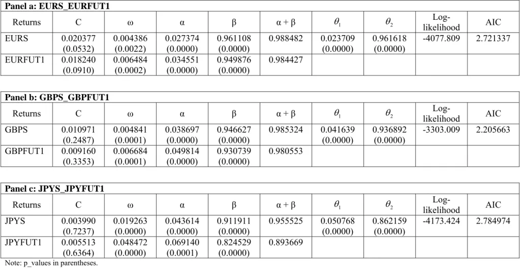
, where Pi,t and Pi,t-1 are the closing prices of currency i for days t and t-1 respectively. In Tables 1, 2 and 3 we show the descriptive statistics for the return series of EUR, GBP and JPY. The mean is close to zero in all cases. For the EUR and JPY currencies the standard deviation of the futures returns is larger than that of the spot returns, indicating the futures market is more volatile than the spot market for these currencies. The exchange rate return series display high kurtosis and heavy tails. Most of them, except EUR, present negative skewness statistics that signify increased presence of extreme losses than extreme gains (longer left tails). The Jarque-Bera Lagrange Multiplier test rejects the null hypothesis of normally distributed returns for every exchange rate series.

[Insert Figure 1]

Figure 1 presents the plot of spot and futures daily returns for each currency. Extremely high positive and negative returns are evident from September 2008 onward, and have continued well into 2009. Therefore, an increase in volatility during the financial crisis is perceived, however, is lower than in other assets (see, f.e., Mc Aleer et al. [46]). In the same way, the plots indicate volatility clustering. Spot and futures returns move in the same pattern suggesting a high correlation (the highest one is between FUT1 and FUT2 for all currencies). Correlations between the returns in European markets (EUR and GBP) are higher than the correlations between these and JPY which is hardly surprising.

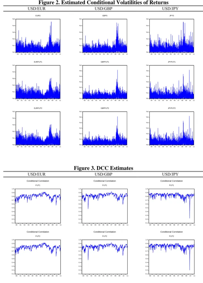
[Insert Figure 2]

(14)

The plots are similar in all returns and the volatility of the series appears to be high during the early 2000s, followed by a quiet period from 2003 to the beginning of 2007. Volatility increases dramatically after August 2008, due in large part to the worsening global credit environment.

(15)

4.- Empirical Results

Estimation Results

We estimate four multivariate models (CCC, VARMA-AGARCH, DCC and BEKK) for each error distribution, currency and two different futures. The estimate underlying parameters are reported in tables 4-7. Table 4 shows the estimates for the CCC model. The volatility persistence, as measure by the sum of   , in either spot or futures markets for each currency is significantly high, ranging from 0.978 to 0.9976, indicating long memory processes. All markets satisfy the second moment and long moment condition, which is a sufficient condition for the QMLE to be consistent and asymptotically normal (see McAleer et.al. [44]) The ARCH and GARCH estimates of the conditional variance are statistically significant. The ARCH estimates are generally small (less than 0.04) and the GARCH effects are generally close to one, finding lower values for the JPY in both spot and futures prices (0.949 and 0.944 against 0.961 and 0.962 for the EUR). There are not big differences among the constant conditional correlation estimates ranging from 0.799 for the EUR to 0.811 for the JPY.

[Insert Table 4] [Insert Table 5]

Table 5 reports the estimates of the conditional mean and variance for the AGARCH models. The ARCH and GARCH effects are statistically significant in all markets and similar to the estimates for the CCC model without asymmetric effects. The asymmetric impact of the unconditional shocks on the conditional variance estimates, ,are weak for the three currencies, in particular are not statistically significant for the JPY.

[Insert Table 6]

The DCC model developed by Engle [24] is employed to capture dynamics conditional correlations. Table 6 summaries the results of the DCC models estimated for all spot and futures markets. Regarding the conditional variance, estimates of all parameters are statistically significant and satisfy the condition   1.The estimates of the DCC

(16)

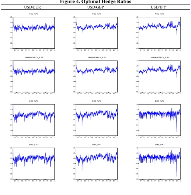
parameters, ˆ₁and ˆ ,₂ are statistically significant for all the currencies. These results suggest that the conditional correlation is not constant over time. The short run persistence of shocks on the dynamic conditional correlation is greater for the JPY at 0.051, although it shows the lower long run persistence of shocks to the conditional correlation 0.913 (0.051+0.862). The EUR shows the lowest short run persistence (0.024) and the greatest long run persistence 0.986 (0.024+0.962). The time-varying conditional correlations between spot and futures returns are given in figure 3. An apparent change in the conditional correlation appeared upon the bankruptcy of Lehman Brothers in New York on 15 September 2008. Due to an increase in the volatility of spot and futures exchange rates, the conditional correlations seem to change in all the currencies. The GFC caused an apparent decline in the conditional correlation between the spot and both FUT1 an FUT2.

[Insert Table 7]

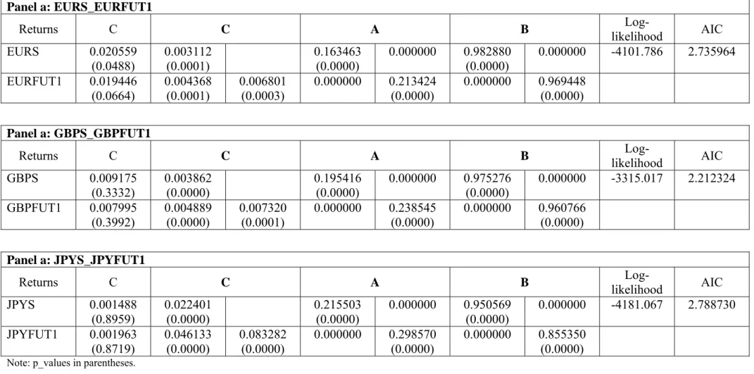
Table 7 reports the estimates for the BEKK model. We have restricted the bivariate BEKK model to the reduced form of the diagonal BEKK. The elements of the covariance matrix depend only on past own squared residuals, and the covariances depend only on past own gross products of residuals. The estimates show that the mean of the returns is not statistically significant. The elements of the diagonal matrices, A and B, are statistically significant. From the empirical results we conclude a time variation in market risk, a strong evidence of GARCH effect and the presence of a weak ARCH effect. The results for the covariance equations are similar, indicating that there is a statistically significant covariation in shocks, which depends more on its lag than on past innovations. These results clearly mean that market shocks are influenced by information which is common to spot and future markets, and as a result of this we have statistically significant covariance in the variance-covariance equations. Model estimations for FUT2 contracts has been done (available upon request) with similar results for the parameters estimates.

(17)

With the estimated underlying parameters in the models, we first generate in-sample daily time series of variance and covariance of the spot and futures returns for each currency. Subsequently, we calculate OHRs and optimal portfolios weights given by equations (14) and (16) respectively.

[Insert Table 8A] [Insert Table 8B] [Insert Table 8C]

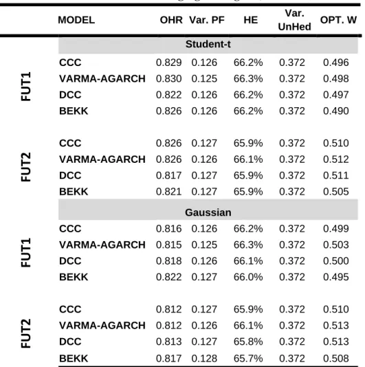
Tables 8A-8C report the average OHR values, the hedge effectiveness, the variance of the portfolio, the hedging effectiveness along with the average value of the optimal portfolio weights for the three currencies using FUT1 and FUT2 contracts when both student’s t and normal error distribution are assumed. We show the results for the four multivariate variance models.

Tables 8A-8C show that hedging is effective in reducing the risks for every model, currency and maturity. In particular, we find that the average OHR using FUT2 contracts are slightly higher than when FUT1 contracts are used, except for the GBP. The highest average OHR value is 0.854 for the USD/JPY when FUT2 contracts are used, meaning that in order to minimize risk, a long (buy) position of one dollar in such a currency should be hedged by a short (sell) position of $0.854 in JPYFUT2 contracts. Additionally, when using Gaussian error distribution tables 8A-8C report lower average OHR values for the three currencies analyzed. The average OHRs from each model are not particularly different, slightly smaller for the DCC and BEKK models when the

Student’s t is used but bigger for the GBP and JPY when using Gaussian distribution. Apparently, the average OHR values are higher for the USD/JPY exchange rate. On the contrary, hedging effectiveness is higher for the DCC and BEKK models.

For the GBP and JPY we notice that hedging effectiveness is slightly higher when a FUT1 contract is used, as opposed to showing a higher hedging effectiveness when the EURFUT2 contract is used. We find a hedging effectiveness that falls between a maximum of 66.3% for the USD/GBP currency and a minimum of 62.5% for the USD/EUR. It seems that hedging effectiveness is slightly higher for the USD/GBP

(18)

[Insert Figure 3] [Insert Figure 4]

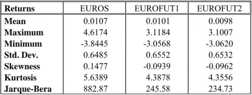
Figure 3 shows the DCC estimates between spot and futures exchange rates for both future contracts. The volatility of the dynamic correlations increases during GFC and, as expected, during turbulent periods correlations decreases. This is why OHR volatility increases during the Global Financial Crisis (GFC). Figure 4 represents the calculated time-varying OHRs from every multivariate conditional volatility model. There are clearly time-varying ratios. It is interesting to look at the optimal hedging ratios during the GFC, for all the models but DCC optimal hedging ratios seem to increase in average.

As showed in the optimal portfolio weight columns in Tables 8A-8C, there are not big differences among models. For example, the largest average value corresponds to a portfolio including the JPYFUT1 contract, which spot currency weight is calculated using the DCC model assuming normal error distribution. The value 0.566 would imply that investors should have more spot currency than futures contracts in their portfolio in order to minimize risk without lowering expected returns. In particular, the optimal holding of one USD/JPY spot/future portfolio is 56.6 cents for spot and 43.4 cents for futures. When Gaussian distribution is used we find higher optimal portfolio weights. For both USD/EUR and USD/JPY spot/futures portfolios the optimal holding of spot currencies is higher when hedging with FUT1 contracts than when FUT2 are used. This is the opposite of what happen for USD/GBP spot/futures portfolios. Estimates suggest holding spot more than GBPFUT1, whereas they suggest holding spot less than GBPFUT2 on one dollar spot/future portfolio.

Summarising estimates based on both OHR and optimal weight values recommend holding more FUT2 than FUT1 contracts for USD/EUR and USD/JPY spot/futures portfolios, meaning that we should increase the percentage of futures contracts for longer term portfolios when these currencies are used.

(19)

5. Conclusions

This study sheds light on the importance of measuring conditional variances and covariances when hedging daily currency risk using futures. The findings are of importance to currency hedgers who require taking futures positions in order to adequately reduce the risk. In this paper, we use four multivariate GARCH models, CCC, VARMA-AGARCH, DCC, and BEKK, to examine the volatilities among spot and two distinct maturity futures, near-month and next-to-near-month contracts. The estimated conditional covariances matrices from these models were used to calculate the optimal portfolios weights and optimal hedge ratios.

The empirical results in this paper reveal that there are not big effectiveness differences when either the near-moth or the next-to-near-month contract is used for hedging spot position on currencies. They even reveal that hedging ratios are lower for near-month contract when the USD/EUR and USD/JPY exchange rates are analyzed. This result is explained in terms of the higher correlation between spot prices and the next-to-near-month futures prices than that with near-next-to-near-month contract and additionally because of the lower volatility of the long maturity futures.

Finally, CCC and VARMA-AGARCH models provide similar results in terms of hedging ratios, portfolio variance reduction and hedging effectiveness. Some differences appear when the DCC and BEKK models are used. Hedging ratios seem to decrease during the GFC as opposed to increasing ratios when CCC and VARMA-AGARH models are consider for calculating the covariance matrix. Future research should be done to investigate the effects of the GFC on the conditional correlation between spot and futures contracts as well as its impact on hedging effectiveness.

(20)

References

[1] P. Araújo Santos, M.I. Fraga Alves, A new class of independence tests for interval forecasts evaluation, Computational Statistics and Data Analysis (2010) in press, doi:10.1016/j.csda2010.10.002.

[2] P. Araújo Santos, Interval forecasts evaluation: R programs for a new independence test, Notas e Comunicações CEAUL 17/2010.

[3] R.T. Baillie, T. Bollerslev, The message in daily exchange rates: a conditionalvariance tale, Journal of Business and Economic Statistics, 7 (1989) 295-307.

[4] R.T. Baillie, R.J Myers, Bivariate GARCH estimation of the optimal commodity futures hedge, Journal of Applied Econometrics, 6 (1991) 109-124.

[5] A.A. Balkema, L. de Haan, Residual life time at great age, Annals of Probability, 2 (1974) 792-804.

[6] L. Bauwens, S. Laurent, J. Rombouts, Multivariate GARCH models: A survey, Journal of Applied Economics, 21 (2006) 79-109.

[7] F. Black, Studies of stock market volatility changes, 1976 Proceedings of the American Statistical Association, Business and Economic Statistics Section, 177-181.

[8] T. Bollerslev, Generalised autoregressive conditional heteroscedasticity, Journal of Econometrics, 31 (1986) 307-327.

[9] T. Bollerslev, A conditional heteroscedastic time series model for speculative prices and rates of return, Review of Economics and Statistics, 69 (1987) 542-547.

[10] T. Bollerslev, Modelling the coherence in short-run nominal exchange rates: a multivariate generalized ARCH model, Review of Economics and Statistics, 72 (1990) 498–505.

[11] H. Bystrom, Managing extreme risks in tranquil and volatile markets using conditional extreme value theory, International Review of Financial Analysis, 13 (2) (2004) 133-152.

[12] M. Caporin, M. McAleer, Scalar BEKK and indirect DCC, Journal of Forecasting, 27 (2008) 537-549.

[13] M. Caporin, M. McAleer, The Ten Commandments for managing investments, Journal of Economic Surveys, 24 (2010a)196-200.

(21)

[14] M. Caporin, M. McAleer, to appear in L. Bauwens, C. Hafner and S. Laurent (eds.), Model selection and testing of conditional and stochastic volatility models, Handbook on Financial Engineering and Econometrics: Volatility Models and Their Applications, Wiley, New York, (2010b) (Available at SSRN: http://ssrn.com/abstract=1676826).

[15] A. Chakraborty, J.T. Barkoulas, Dynamic futures hedging in currency markets, The European Journal of Finance, 5 (1999) 299-314.

[16] W.H. Chan, Dynamic Hedging with Foreign Currency Futures in the Presence of Jumps, Studies in Nonlinear Dynamics & Econometrics, V. 12, Issue 2 (2008) 1-24.

[17] C.L. Chang, M. Mc Aleer, R. Tansuchat, Crude oil hedging strategies using dynamic multivariate GARCH, Energy Economics, 33(5) (2011) 912-923.

[18] P. Christoffersen P., Evaluating intervals forecasts, International Economic Review, 39 (1998) 841-862.

[19] F.X. Diebold, Empirical Modeling of Exchange Rate Dynamics, Springer Verlag, New York, 1988.

[20] F.X. Diebold, T. Schuermann, J.D. Stroughair, Pitfalls and opportunities in the use of extreme value theory in risk Management, Working Paper, (1998) 98-10, Wharton School, University of Pennsylvania.

[21] L.H. Ederington, The hedging performance of the new futures markets, Journal of Finance, 34 (1979) 157-170.

[22] P. Embrechts, C. Klüppelberg, T. Mikosch, Modeling extremal events for insurance and finance, Springer, Berlín, 1997.

[23] R.F. Engle, Autoregressive conditional heteroscedasticity with estimates of the variance of United Kingdom inflation, Econometrica, 50 (1982) 987-1007.

[24] R.F. Engle, Dynamic conditional correlation: A simple class of multivariate generalized autoregressive conditional heteroskedasticity models, Journal of

Business and Economic Statistics, 20 (2002) 339-350.

[25] R.F. Engle., K.F. Kroner, Multivariate simultaneous generalized ARCH, Econometric Theory, 11 (1995) 122-150.

[26] P.H. Franses, D. van Dijk, Nonlinear Time Series Models in Empirical Finance, Cambridge University Press, Cambridge, 1999.

(22)

[28] L. Glosten, R. Jagannathan, D. Runkle, On the relation between the expected value and volatility of nominal excess return on stocks, Journal of Finance, 46 (1992) 1779-1801.

[29] A. Hakim, M. McAleer, Forecasting conditional correlations in stock, bond and foreign exchange markets, Mathematics and Computers in Simulation, 79 (2009) 2830–2846.

[30] S. Haqmmoudeh, Y. Yuan, M. McAleer, M.A. Thomson, M.A., Precious metals-exchange rate volatility transmissions and hedging strategies, International Review of Economics and Finance, 19 (2010) 633-647.

[31] A.F. Herbs, D.D. Kare, J.F. Marshall, A time varying convergence adjusted, minimum risk futures hedge ratio, Advances in futures and option research, vol. 6 April (1993) 137-155.

[32] L.L. Johnson, The theory of hedging and speculation in commodity futures, Review of Economic Studies, 27 (1960) 139-151.

[33] K.F. Kroner, V. Ng, Modelling asymmetric movements of asset prices, Review of Financial Studies, 11 (1998) 844-871.

[34] K.F. Kroner, J. Sultan, in S.G. Rhee and R.P. Change (eds.), Foreign currency futures and time varying hedge ratios, Pacific-Basin Capital Markets Research, Vol. II, Amsterdam North-Holland, pp. 397-412, 1991.

[35] K.F. Kroner, J. Sultan, Time-varying distributions and dynamic hedging with foreign currency futures, Journal of Financial and Quantitative Analysis, 28 (1993) 535-551.

[36] P. Kupiec, Techniques for verifying the accuracy of risk measurement models, Journal of Derivatives, 3 (1995) 73-84.

[37] Y.H. Ku, H.C. Chen, K.H. Chen, (2007), On the application of the dynamic conditional correlation model in estimating optimal time-varying hedge ratios, Applied Economics Letters, 14 (2007) 503-509.

[38] W.K. Li, S. Ling, M. McAleer, M., Recent theoretical results for time series models with GARCH errors, Journal of Economic Surveys, 16 (2002) 245-269. Reprinted in M. McAleer and L. Oxley (eds.), Contributions to Financial Econometrics: Theoretical and Practical Issues, Blackwell, Oxford, pp. 9-33. [39] D. Lien, Y.K. Tse, A.K. Tsui, Evaluating the hedging performance of the

(23)

[40] S. Ling, M. McAleer, Stationarity and the existence of moments of a family of GARCH processes, Journal of Econometrics, 106 1 (2002a) 9-117.

[41] S. Ling, M. McAleer, Necessary and sufficient moment conditions for the GARCH(r,s) and asymmetric power GARCH(r, s) models, Econometric Theory, 18 (2002b) 722-729.

[42] S. Ling, M. McAleer, Asymptotic theory for a vector ARMA-GARCH model, Econometric Theory, 19 (2003) 278-308.

[43] M. McAleer, Automated inference and learning in modelling financial volatility, Econometric Theory, 21 (2005) 232-261.

[44] M. McAleer, F. Chan, F., D. Marinova, An econometric analysis of asymmetric volatility: theory and application to patents, Journal of Econometrics, 139 (2007) 259-284.

[45] M. McAleer, S. Hoti, F. Chan, Structure and asymptotic theory for multivariate asymmetric conditional volatility, Econometric Reviews, 28 (2009) 422-440. [46] M. McAleer, J.A. Jiménez-Martín, T. Pérez- Amaral, T., International Evidence on

GFC-robust Forecasts for Risk Management under the Basel Accord, 2011 (Available at SSRN: http://papers.ssrn.com/sol3/papers.cfm?abstract_id=1741565) [47] A.J. McNeil, R. Frey, Estimation of tail-related risk measures for heteroscedastic financial time series: An extreme value approach, Journal of Empirical Finance, 7 (2000) 271-300.

[48] D.B. Nelson, Conditional heteroscedasticity in asset returns: A new approach, Econometrica, 59 (1991) 347-370.

[49] J. Pickands III, Statistical inference using extreme value order statistics, Annals of Statistics, 3 (1975) 119-131.

[50] R.D. Ripple, I.A. Moosa, Hedging effectiveness and futures contract maturity: the case of NYMEX crude oil futures, Applied Financial Economics, 17 (2007) 683-689.

[51] Riskmetrics, J.P. Morgan Technical Document, 4th Edition, J.P. Morgan, New York, 1996.

[52] R Development Core Team, A language and environment for statistical computing. R Foundation for Statistical Computing, Vienna, Austria, 2008. ISBN 3-900051-07-0, URL http://www.R-project.org.

(24)

Econometrics, Finance and Other Fields, Chapman & Hall, London, 1996, pp. 1-67.

[54] R. Smith, Estimating tails of probability distributions. Annals of Statististics, 15 (1987) 1174-1207.

[55] G. Stahl, Three cheers, Risk, 10 (1997) 67-69.

[56] J.L. Stein, The simultaneous determination of spot and futures prices, American Economic Review, 51 (1961) 1012-1025.

[57] G. Zumbauch, A Gentle Introduction to the RM 2006 Methodology, Riskmetrics Group, New York, 2007.

(25)

Figure 1. Spot and futures daily returns

USD/EUR USD/GBP USD/JPY

-4% -3% -2% -1% 0% 1% 2% 3% 4% 5% 00 01 02 03 04 05 06 07 08 09 10 11 EURS -4% -3% -2% -1% 0% 1% 2% 3% 4% 5% 00 01 02 03 04 05 06 07 08 09 10 11 GBPS -5% -4% -3% -2% -1% 0% 1% 2% 3% 4% 00 01 02 03 04 05 06 07 08 09 10 11 JPYS -4% -3% -2% -1% 0% 1% 2% 3% 4% 00 01 02 03 04 05 06 07 08 09 10 11 EUROFUT1 -6% -4% -2% 0% 2% 4% 00 01 02 03 04 05 06 07 08 09 10 11 GBPFUT1 -6% -4% -2% 0% 2% 4% 6% 00 01 02 03 04 05 06 07 08 09 10 11 JPYFUT1 -4% -3% -2% -1% 0% 1% 2% 3% 4% 00 01 02 03 04 05 06 07 08 09 10 11 EUROFUT2 -6% -4% -2% 0% 2% 4% 00 01 02 03 04 05 06 07 08 09 10 11 GBPFUT2 -6% -4% -2% 0% 2% 4% 6% 00 01 02 03 04 05 06 07 08 09 10 11 JPYFUT2

(26)

Figure 2. Estimated Conditional Volatilities of Returns

%0 %1 %2 %3 %4 %5 00 01 02 03 04 05 06 07 08 09 10 11 EURS %0 %1 %2 %3 %4 %5 00 01 02 03 04 05 06 07 08 09 10 11 GBPS %0 %1 %2 %3 %4 %5 00 01 02 03 04 05 06 07 08 09 10 11 JPYS %0 %1 %2 %3 %4 %5 00 01 02 03 04 05 06 07 08 09 10 11 EURFUT1 %0 %1 %2 %3 %4 %5 %6 00 01 02 03 04 05 06 07 08 09 10 11 GBPFUT1 %0 %1 %2 %3 %4 %5 %6 00 01 02 03 04 05 06 07 08 09 10 11 JPYFUT1 %0 %1 %2 %3 %4 %5 00 01 02 03 04 05 06 07 08 09 10 11 EURFUT2 %0 %1 %2 %3 %4 %5 %6 00 01 02 03 04 05 06 07 08 09 10 11 GBPFUT2 %0 %1 %2 %3 %4 %5 %6 00 01 02 03 04 05 06 07 08 09 10 11 JPYFUT2 Figure 3. DCC Estimates

0.1 0.2 0.3 0.4 0.5 0.6 0.7 0.8 0.9 1.0 00 01 02 03 04 05 06 07 08 09 10 11 FUT1 Conditional Correlation 0.1 0.2 0.3 0.4 0.5 0.6 0.7 0.8 0.9 1.0 00 01 02 03 04 05 06 07 08 09 10 11 FUT1 Conditional Correlation 0.1 0.2 0.3 0.4 0.5 0.6 0.7 0.8 0.9 1.0 00 01 02 03 04 05 06 07 08 09 10 11 FUT1 Conditional Correlation 0.1 0.2 0.3 0.4 0.5 0.6 0.7 0.8 0.9 1.0 00 01 02 03 04 05 06 07 08 09 10 11 FUT2 Conditional Correlation 0.1 0.2 0.3 0.4 0.5 0.6 0.7 0.8 0.9 1.0 00 01 02 03 04 05 06 07 08 09 10 11 FUT2 Conditional Correlation 0.1 0.2 0.3 0.4 0.5 0.6 0.7 0.8 0.9 1.0 00 01 02 03 04 05 06 07 08 09 10 11 FUT2 Conditional Correlation

(27)

Figure 4. Optimal Hedge Ratios

0.0 0.2 0.4 0.6 0.8 1.0 1.2 00 01 02 03 04 05 06 07 08 09 10 11 CCC_FUT1 0.0 0.2 0.4 0.6 0.8 1.0 1.2 00 01 02 03 04 05 06 07 08 09 10 11 CCC_FUT1 0.0 0.2 0.4 0.6 0.8 1.0 1.2 00 01 02 03 04 05 06 07 08 09 10 11 CCC_FUT1 0.0 0.2 0.4 0.6 0.8 1.0 1.2 00 01 02 03 04 05 06 07 08 09 10 11 VARMA-AGARCH_FUT1 0.0 0.2 0.4 0.6 0.8 1.0 1.2 00 01 02 03 04 05 06 07 08 09 10 11 VARMA-AGARCH_FUT1 0.0 0.2 0.4 0.6 0.8 1.0 1.2 00 01 02 03 04 05 06 07 08 09 10 11 VARMA-AGARCH_FUT1 0.0 0.2 0.4 0.6 0.8 1.0 1.2 00 01 02 03 04 05 06 07 08 09 10 11 DCC_FUT1 0.0 0.2 0.4 0.6 0.8 1.0 1.2 00 01 02 03 04 05 06 07 08 09 10 11 DCC_FUT1 0.0 0.2 0.4 0.6 0.8 1.0 1.2 00 01 02 03 04 05 06 07 08 09 10 11 DCC_FUT1 0.0 0.2 0.4 0.6 0.8 1.0 1.2 00 01 02 03 04 05 06 07 08 09 10 11 BEKK_FUT1 0.0 0.2 0.4 0.6 0.8 1.0 1.2 00 01 02 03 04 05 06 07 08 09 10 11 BEKK_FUT1 0.0 0.2 0.4 0.6 0.8 1.0 1.2 00 01 02 03 04 05 06 07 08 09 10 11 BEKK_FUT1

(28)

Table 1. EUR Descriptive Statistics

Returns EUROS EUROFUT1 EUROFUT2 Mean 0.0107 0.0101 0.0098 Maximum 4.6174 3.1184 3.1007 Minimum -3.8445 -3.0568 -3.0620 Std. Dev. 0.6485 0.6552 0.6532 Skewness 0.1477 -0.0939 -0.0962 Kurtosis 5.6389 4.3878 4.3556 Jarque-Bera 882.87 245.58 234.73

Table 2. GPB Descriptive Statistics

Returns GBPS GBPFUT1 GBPFUT2 Mean -0.0007 -0.0010 -0.0011 Maximum 4.4745 3.3542 3.3147 Minimum -3.9182 -5.1703 -5.1326 Std. Dev. 0.6103 0.6010 0.6021 Skewness -0.0552 -0.3793 -0.3560 Kurtosis 7.3609 6.7628 6.5791 Jarque-Bera 2382.7 1844.9 1667.4

Table 3. JPY Descriptive Statistics

Returns JPYS JPYFUT1 JPYFUT2 Mean -0.0077 -0.0075 -0.0070 Maximum 3.0770 4.0082 4.0187 Minimum -4.6098 -5.1906 -5.2289 Std. Dev. 0.6594 0.6642 0.6594 Skewness -0.4246 -0.3285 -0.3020 Kurtosis 6.5503 6.9307 6.9282 Jarque-Bera 1668.5 1988.5 1977.8

(29)

Table 4. CCC Estimates Panel a: EURS_EURFUT1

Returns C ω α β α + β Conditional Constant

Correlation Log-likelihood AIC EURS 0.025532 (0.0165) 0.001324 (0.1455) 0.036873 (0.0000) 0.960795 (0.0000) 0.997668 0.798867 (0.0000) -4105.754 2.738605 EURFUT1 0.022376 (0.0454) 0.001886 (0.0329) 0.034411 0.0000 0.962024 0.0000 0.996435 Panel b: GBPS_GBPFUT1

Correlation Log-likelihood AIC GBPS 0.014299 (0.1479) 0.002229 (0.0086) 0.030472 (0.0000) 0.962650 (0.0000) 0.993122 0.812791 (0.0000) -3367.432 2.247209 GBPFUT1 0.012066 (0.2202) 0.002608 (0.0055) 0.028671 (0.0000) 0.963302 (0.0000) 0.991973 Panel c: JPYS_JPYFUT1

Correlation Log-likelihood AIC JPYS 0.003894 (0.7283) 0.006035 (0.0269) 0.037076 (0.0000) 0.948975 (0.0000) 0.986051 0.811211 (0.0000) -4239.943 2.827915 JPYFUT1 0.005502 (0.6230) 0.009677 (0.0205) 0.033193 (0.0055) 0.944285 (0.0000) 0.977478

(30)

Table 5. VARMA-AGARCH Estimates Panel a: EURS_EURFUT1 Returns C ω α β γ α+β+γ Constant Conditional Correlation Log-likelihood AIC EURS 0.016007 (0.1350) 0.001446 (0.1021) 0.025002 (0.0027) 0.962974 (0.0000) 0.018713 (0.0489) 1.006689 0.799869 (0.0000) -4098.227 2.734926 EURFUT1 0.011699 (0.2921) 0.002113 (0.0135) 0.020336 (0.0105) 0.964626 (0.0000) 0.021366 (0.0483) 1.006328 Panel b: GBPS_GBPFUT1

Returns C ω α β γ α+β+γ Conditional Constant

Correlation Log-likelihood AIC GBPS 0.004260 (0.6588) 0.002587 (0.0021) 0.014752 (0.0446) 0.963269 (0.0000) 0.027465 (0.0117) 1.005486 0.813575 (0.0000) -3356.194 2.241061 GBPFUT1 0.001990 (0.8368) 0.002791 (0.0021) 0.016439 (0.0301) 0.964716 (0.0000) 0.020035 (0.0644) 1.00119 Panel c: JPYS_JPYFUT1 Returns C ω α β γ α+β+γ Constant Conditional Correlation Log-likelihood AIC JPYS 0.004648 (0.6808) 0.006036 (0.0315) 0.038539 (0.0006) 0.949630 (0.0000) -0.004651 (0.7528) 0.983518 0.811191 (0.0000) -4239.519 2.828964 JPYFUT1 0.005544 (0.6287) 0.009533 (0.0208) 0.032053 (0.0331) 0.944463 (0.0000) 0.002810 (0.8728) 0.979326 Note: p_values in parentheses.

(31)

Table 6. DCC Estimates Panel a: EURS_EURFUT1 Returns C ω α β α + β 1 2 Log-likelihood AIC EURS 0.020377 (0.0532) 0.004386 (0.0022) 0.027374 (0.0000) 0.961108 (0.0000) 0.988482 0.023709 (0.0000) 0.961618 (0.0000) -4077.809 2.721337 EURFUT1 0.018240 (0.0910) 0.006484 (0.0002) 0.034551 (0.0000) 0.949876 (0.0000) 0.984427 Panel b: GBPS_GBPFUT1

Returns C ω α β α + β 1 2 _likelihoodLog- AIC

GBPS 0.010971 (0.2487) 0.004841 (0.0001) 0.038697 (0.0000) 0.946627 (0.0000) 0.985324 0.041639 (0.0000) 0.936892 (0.0000) -3303.009 2.205663 GBPFUT1 0.009160 (0.3353) 0.006684 (0.0001) 0.049814 (0.0000) 0.930739 (0.0000) 0.980553 Panel c: JPYS_JPYFUT1

Returns C ω α β α + β 1 2 _likelihoodLog- AIC

JPYS 0.003990 (0.7237) 0.019263 (0.0000) 0.043614 (0.0000) 0.911911 (0.0000) 0.955525 0.050768 (0.0000) 0.862159 (0.0000) -4173.424 2.784974 JPYFUT1 0.005513 (0.6364) 0.048472 (0.0000) 0.069140 (0.0001) 0.824529 (0.0000) 0.893669 Note: p_values in parentheses.

(32)

Table 7. BEKK Estimates Panel a: EURS_EURFUT1

Returns C C A B _likelihoodLog- AIC

EURS 0.020559 (0.0488) 0.003112 (0.0001) 0.163463 (0.0000) 0.000000 0.982880 (0.0000) 0.000000 -4101.786 2.735964 EURFUT1 0.019446 (0.0664) 0.004368 (0.0001) 0.006801 (0.0003) 0.000000 0.213424 (0.0000) 0.000000 0.969448 (0.0000) Panel a: GBPS_GBPFUT1 Returns C C A B Log-likelihood AIC GBPS 0.009175 (0.3332) 0.003862 (0.0000) 0.195416 (0.0000) 0.000000 0.975276 (0.0000) 0.000000 -3315.017 2.212324 GBPFUT1 0.007995 (0.3992) 0.004889 (0.0000) 0.007320 (0.0001) 0.000000 0.238545 (0.0000) 0.000000 0.960766 (0.0000) Panel a: JPYS_JPYFUT1

Returns C C A B _likelihoodLog- AIC

JPYS 0.001488 (0.8959) 0.022401 (0.0000) 0.215503 (0.0000) 0.000000 0.950569 (0.0000) 0.000000 -4181.067 2.788730 JPYFUT1 0.001963 (0.8719) 0.046133 (0.0000) 0.083282 (0.0000) 0.000000 0.298570 (0.0000) 0.000000 0.855350 (0.0000) Note: p_values in parentheses.

(33)

Table 8A. Alternative hedging strategies (USD/EUR)

MODEL OHR Var. PF HE

Var. UnHed OPT. W Student-t

FUT1

CCC 0.805 0.158 62.5% 0.420 0.536 VARMA-AGARCH 0.805 0.157 62.7% 0.420 0.536 DCC 0.794 0.157 62.7% 0.420 0.542 BEKK 0.802 0.157 62.6% 0.420 0.542

FUT2

CCC 0.808 0.157 62.7% 0.420 0.532 VARMA-AGARCH 0.808 0.156 62.9% 0.420 0.532 DCC 0.797 0.156 62.9% 0.420 0.535 BEKK 0.804 0.156 62.8% 0.420 0.537 Gaussian

FUT1

FUT2

Notes: Optimal Hedging Ratio (OHR), Variance of Portfolios (Var. PF), Hedging Effective Index

(34)