Has Moral Hazard Become a More Important Factor in
Managerial Compensation?
∗
George-Levi Gayle
Tepper School of Business, Carnegie Mellon University
Robert A. Miller
Tepper School of Business, Carnegie Mellon University
November 7, 2005
Abstract
The theory of moral hazard predicts that since the activities of managers are hard to monitor directly, managerial compensation is tied to the profitability of the firms they manage. In this empirical study we investigate the hypothesis that the secular trends in managerial compensation can be attributed to the changing importance of moral hazard that affect the optimal contract through shifts in the distribution of the abnormal returns to thefirm. We estimate a principal agent model of moral hazard controlling for heterogeneity across sectors, different measure of firm size, leverage, and executive position within the firm hierarchy. Our two data sets on three industrial sectors, which together span a sixty year period, strengthens past research that documents the increasing level of total executive compensation and the sensitivity of compensation tofirm performance over the last two decades.
Within each data set almost all variation in executive compensation is explained by the firms abnormal returns and the controls in our empirical model. We find that had moral hazard not been a factor, compensation in the three sectors would have increased at the same rate as national income, much lower than the average increase that actually occurred. Wefind little evidence to suggest that managerial tastes have changed, or that the nonpecuniary benefits to managers deviating from shareholder interests have increased. There are two factors driving the sharply increased costs of moral hazard. First, increased dispersion of abnormal returns has led to deterioration in the signal shareholders receive about managerial activities, raising the welfare costs of moral hazard in two sectors we investigate. Second, wefind the changing composition offirms in all sectors has increased averagefirm size, and wefind that managing largerfirms increases the discrepancy between shareholder and managerial interests.
1
Introduction
Managers are paid to organize human resources in creative ways that add value to their firm.
Because their activities are hard to monitor, managers are rarely paid for their inputs. Execu-tive compensation is instead tied to various indicators of managerial effort, such as theirfirm’s
performance. Linking a manager’s compensation to the firm’s performance requires him (or,
in rare cases, her) to hold a substantial amount of personal wealth in assets that are sensitive
to the firm’s performance, such as its stocks and options, thus preventing the manager from
holding a more diversified portfolio that insulates him against the abnormal returns of his own
firm. Called moral hazard, this is the main reason labor economists and contract theorists
give to explain why managers are not paid like most other professionals, at a rate more or less equalized across a large market for similarly skilled workers after adjusting for cost of living
and amenity indices.1
The dramatic increase in both the level of CEO compensation and its sensitivity to firm
performance over the last quarter century is widely documented by Brian Hall and Jeffrey
Liebman (1998) and Kevin Murphy (1999). Those studies show that, of all the components
making up executive pay, including cash and bonus, stock grants, retirement benefits, the
biggest increases have been in option grants. Thus much of the increase in managerial com-pensation is attributable to increases in asset grants whose value is explicitly tied to the value
of the firm. Since moral hazard explains why managerial compensation andfirm performance
should be connected, it is tempting to suggest that changes in the nature of moral hazard might have triggered these trends. Our study formulates this suggestion as a hypothesis and
tests it with data on managerial compensation and abnormal returns to theirfirms.
In Section 2 we define three measures of moral hazard in management, the loss in firm
value from not contracting with a manager to overcome the moral hazard problem, the gain to managers from putting their personal goals ahead of theirfirm’s, and a shadow value of afirm’s willingness to pay for monitoring technology that would eliminate moral hazard. This shadow value reflects the quality of the signal shareholders receive about the choices and strategies of
management, generated by the firm’s probability distribution for abnormal returns that are
ultimately determined by the firm’s technology. The third section develops a principal agent
model of moral hazard to identify the parameters which determine these three measures. Our empirical analysis, described in Section 4, is based on two data sets of comparable size onfirms in three industrial sectors that span approximately sixty years and, as we show, are broadly representative of all publicly traded firms.3
We describe the nonlinear estimation techniques to obtain consistent estimators of those parameters from the optimal contract solution to the structural model in Section 5. Our main
findings are reported in Section 6. We find that because the average firm size has greatly
increased, losses to firms from ignoring the moral hazard problem and writing contracts that
do not incentive managers have substantially increased too. There is little evidence to suggest that the preferences of managers are more disposed to acting against shareholder interests. In the absence of moral hazard our model predicts that the compensation of managers over this period would have increased at the same rate as national income. Thus tastes have not
changed significantly over this period, so cannot provide an explanation for the trends in managerial compensation. Nevertheless our model explains about 90 percent of the variation in managerial compensation in each data set. Our results shows that the increased shadow value of moral hazard explains most of the trend in managerial compensation. The remainder
is accounted for by rising living standards over the past 60 years. Finally we find that the
increased shadow value is due to the deteriorating quality of signals that shareholders receive
about the manager’s work effort, and is synonymous with the idea that managing firms has
become more complex.
2
Measuring Moral Hazard
Arguing that "agency theory remains the only viable candidate for the answer to the question "How well does executive compensation work?" John Abowd and David Kaplan (1999) re-cently posed six questions about executive compensation that need answering. Our measures, borrowed from Margiotta and Miller (2000), directly relate to three of them: "How much
does executive compensation cost thefirm?" . . . How much is executive compensation worth
to the recipient? . . . What are the effects of executive compensation?". We characterize
the importance of moral hazard three ways, the gross loss shareholders would incur (before accounting for managerial compensation) from the manager tending his own interests, the
benefits accruing to the manager from tending his own interests instead of his shareholders’,
and how much the shareholders are willing to pay to eliminate the problem of moral hazard altogether.
The first measure, denotedτ1,is the expected gross output loss to thefirm switching from
the distribution of abnormal returns for the diligent work to the distribution for shirking, that
is the difference between the expected output to the plant from the manager pursuing the
firm’s goals versus his or her own, before netting out expected managerial compensation. Let
v denote the value of the firm at the beginning of the period, and let x denote the firm’s
abnormal return realized at the end of the period. Following literary convention, we describing
a manager who pursues the interests of the firm as working, and a manager who pursues his
own interests, when compensation is independent of firm performance, as shirking. Then:
τ1 = E[x|manager works]v−E[x|manager shirks]v
= −E[x|manager shirks]v
where the second equality exploits the identity that the expected value of abnormal returns is
zero when the manager is pursuing the interests of thefirm.
The second measure, τ2,is the nonpecuniary benefits to the manager from shirking, that
is pursuing his own goals within the firm. Let w2 denote the manager’s reservation wage to
work under perfect monitoring or if there were no moral hazard problem, and let w1 denote
the manager’s reservation wage to shirk. Thenτ2, the compensating differential for these two
activities, can be expressed as the difference:
We also estimate the maximum amount shareholders are willing pay to eliminate the moral
hazard problem, the value of a perfect monitor. Absent moral hazard, the firm would pay
the manager the fixed wage w2, instead of according to the compensation w(x). The firms’
willingness to pay for eliminating the moral hazard problem, denotedτ3,is accordingly defined
as:
τ3=E[w(x)]−w2 (1)
This measure is actually a lower bound on the shareholders willingness to pay for perfect monitor, because it is based on asking the manager to perform the same tasks. If, however, the manager’s actions could be monitored perfectly, it is plausible that shareholders would modify
the manager’s job description to better exploit the monitoring technology for the benefit of
thefirm, an issue analyzed in Prendergast (2002).
Against the output reduction from shirking τ1,is the savings in managerial compensation
coming from two terms, the shadow value of a perfect monitor, and the cost of inducing
the manager to work diligently when a perfect monitor is removed. Subtracting from τ1 the
sum of τ2 and τ3, we obtain the net income loss a firm would sustain from signing a shirking
contract with a manager. This net amount represents the value of preventing the manager from undoing contracts that align his incentives with thefirm, by dealing with a lender who does not
recognize the folly of allowing the manager to insure himself against poor firm performance,
and is unaware of public disclosure laws that require the manager to report his holdings offirm related securities.
3
A Model
This section lays out a theoretical principal-agent framework on which our empirical analysis
is based.3 At each time period t, there are three activities in which a person can be engaged,
working as the firm manager in the shareholders’ interests, being employed as a manager at
the firm but pursuing different interests to the shareholders, or not engaged by thefirm. Let lt≡(l0t, l1t, l2t)denote the three possible activities, whereljt ∈{0,1}is an indicator for choice j∈{1,2,3} and
j=2
X j=0
ljt = 1
If l0t = 1, we say that the manager is not engaged by the firm and this activity is publicly
observed,l1t= 1denotes shirking and l2t= 1denotes working diligently. While l0tis common knowledge the values of (l1t, l2t) are hidden from the shareholders. Apart from choosing his
activity, the manager also chooses his consumption for the period. Letctdenote the manager’s
consumption in periodt. We assume that preferences over consumption and work are
parame-terized by a utility function exhibiting absolute risk aversion that is additively separable over periods and multiplicatively separable with respect to consumption and work activity within periods. In the model we estimate, lifetime utility can be expressed as:
where β is the constant subjective discount factor, αj are utility parameters associated with
setting ljnt = 1 and ρ is the constant absolute level of risk aversion. We set α0 = 1 as a
normalization, since behavior is invariant to linear transformation of the utility function under
the independence axiom. We assume thatα2 > α1,or that diligence is more distasteful than
shirking. This assumption is the vehicle by which the manager’s preferences are not aligned with shareholders interests. We are not suggesting that managers are inherently lazy, merely
that their personal goals do not motivate them to maximize the value of the firm if their
compensation is independent of the firm’s performance. Finally we requireα1 >0 to ensure
utility is increasing in consumption.
In the optimal contract shareholders induce their manager to bear risk on only that part of the return whose probability distribution is affected by his actions. Since managers are risk averse (an assumption we test empirically), his certainty equivalent for a risk bearing security is less than the expected value of security, so shareholders would diversify amongst themselves
everyfirm security whose returns are independent of the manager’s activities, rather than use
it to pay the manager. We define the abnormal returns of thefirm as the residual component of returns that cannot be priced by aggregate factors the manager does not control. In an optimal contract compensation to the manager might depend on this residual in order to provide him with appropriate incentives, but it should not depend on changes in stochastic factors that
originate outside the firm, which in any event can be neutralized by adjustments within his
wealth portfolio through the other stocks and bonds he holds.
More specifically, let wt denote the overall compensation received by the manager at the
end of periodtas compensation for work done during the period, and vt the value of thefirm
at that point in time. Then the gross abnormal return attributable to the manager’s actions is the residual
xt≡
vt+wt−vt−1
vt−1 −
πt−ztγ
whereπtis the difference between the return on the market portfolio in periodtand the return on the firm’s stock, andztγ is a linear combination of some risk factors, denotedzt,that lead
to systematic deviations between the the expected return on thefirm’s shares and the market
portfolio. This study assumes that xt is a random variable that depends on the manager’s
effort activity choice in the previous period but, conditional on(l1t, l2t), is independently and identically distributed across both firms and periods. Givenljt = 1, for j ∈{1,2}, we denote the probability density function ofxt by fj(xt).
The measures of moral hazard described in the previous section can be derived as functions
of the parameters defining this framework. The expected loss per period to thefirm from the
manager pursuing his own interests rather than value maximization is : τ1 =−v
Z
xf1(x)dx
where v is the value of the firm in the previous period. The compensating differential to the
derived directly from the manager’s utility function: τ2 =ρ−1log µ α2 α1 
In contrast to the other two measures, the welfare cost of moral hazard depends on the optimal contract. It is the expected value of managerial compensation, less its certainty equivalent:
τ3= Z w(x)f2(x)dx−ρ−1log µ α2 α0 
The value of being able to offer a contract that creates the manager’s incentive to work, as
opposed to paying him afixed wage, is thus:
τ1−τ2−τ3=ρ−1log µ α1 α0 ¶ −v Z xf1(x)dx− Z w(x)f2(x)dx
Within this model there arefive parameters that might account for differences in executive
compensation, that is apart from thefirm’s abnormal return. They are the probability
distri-bution of abnormal returns conditional on working, the probability distridistri-bution of abnormal
returns conditional on shirking, the risk aversion parameter, the nonpecuniary benefit from
shirking versus working, and the nonpecuniary benefit of working versus retiring or accepting
employment outside the firm. The first two production parameters, f2(x) and f1(x),
deter-mine τ1, three of the taste parameters, ρ and α2/α1, are used to define τ2, and as our brief
discussion of the optimal contract shows below, all the parameters affect τ3. Our empirical
analysis allows each parameter to differ across firm type and executive position. We also
con-sider the possibility that thefive parameters have changed over time, and that they depend on
underlying factors whose values have changed. In this way we seek to discover why managerial
compensation has increased and become more diffuse over the past 60 years.
4
Data
We used two sources of compensation and returns data to construct three samples for our
empirical study. Thefirst source of compensation was originally collected by Masson (1971)
and later extended by Antle and Smith (1985,1986). They contain compensation data on the top three executives of 37firms for the period 1948 through 1977. A detailed description of the
first data set can be obtained from Antle and Smith (1985). The primary source for the other
two samples is the June 2004 version of the S&P ExecuComp database. This database follows
the 2,610 firms in the S&P 500, Midcap, and Smallcap indices and contains information on
the eight highest-paid executives. We supplemented these data with firm level data obtained
from the S&P COMPUSTAT North America database and monthly stock price data from the Center for Securities Research (CSP) database.
Thefirst data set contains compensation data for three industrial sectors, namely, aerospace, chemicals and electronics. To ensure comparability of our results across the two time periods
we constructed two separate samples from the second data set. The first sample is made of
firms that belong to the three sectors contain in the first data set, that is according to the
International Industrial Classification code. The second sample includes allfirms in the S&P
ExecuComp database. The first two samples allow us to directly compare the behavior of
executive compensation across the two time periods controlling for aggregate conditions in the
economy, and measures of the size and capital structure of firms. The third sample allows us
to discern whether our restricted sample is broadly representative of the whole population of
firms in economy or not.
To facilitate comparisons across the three samples, in the two more recent samples we deleted observations on female executives, and retained only the top three executives, since there are no female executives in the older sample, and no information on executives below the top three. We deleted observations with missing information, such as where compensation
is reported for executives who had held the office for less that 50 weeks of a given year, and
we also eliminated observations where the same executive is simultaneously listed with more
than one company. This left us with 151 firms and 4,150 observation in the second sample,
and 1,517 firms and 82, 578 observations in the third sample.
4.1
Abnormal returns
We computed two measures of xt, gross abnormal returns to the firm in period t. First we
computed the difference between the return on an asset and the return on the market portfolio.
Then we regressed the difference on factors that systematically vary with the first measure,
including sector specific constant and GDP. The sample means of the residual and its standard
deviation are displayed in Table 1. (The inclusion of a constant in the regression guarantees that the sample mean of the second residual is numerically zero.)
table 1
Two measures of abnormal returns (standard deviations in parenthesis)
Interpreting the first measure of abnormal returns as a random variable, we cannot reject
the null hypothesis that in all three data sets, it has mean zero. All the coefficients in the
regression run to form the second measure of abnormal returns proved significant, but including the extra factors affects their dispersion by only a trivial amount, as can be seen by comparing the respective second moments. Regardless of which measure is used, dispersion has increased in the chemicals and electronics sectors, but has declined in the aerospace sector. Dispersion in the unrestricted sample is higher than in the old sample of three sectors, but lower than in the new restricted sample. In the presentation that follows we have only reported results
obtained using the second measure of abnormal returns, but results obtained using the first
4.2
Firm characteristics
The characteristics of the manager’s firm affects the nature of his responsibilities and the
satisfaction he derives from his job. These characteristics are also relevant to the nonpecuniary satisfaction derived from pursuing his own goals within the firm.4 Table 2 is a cross sectional summary of the characteristics we used in estimation.
Table 2
cross-sectional information on sectors in millions of $us 2000 (standard deviations in parenthesis)
We partitioned each data set by sector and focused on four indicators of size, namely sales, value of equity, total assets and number of employees. These indicators convey some idea of the scope of managerial responsibilities. Sales have almost tripled in the three sectors, rising
by less than a factor of two in chemicals, but by more than five in the other two sectors.
Average sales per firm in these three sectors is about three quarters of average sales in the
unrestricted sample of all listed firms. Similar changes in magnitude apply to equity value.
However all sectors have become much more capital intensive, as gauged by changes in total assets and employment. Assets have increased more than tenfold in aerospace and electronics, and by more than a factor of four in chemicals. Employment has declined in two out of the
three sectors, most markedly in chemicals, where the average firm employs less than half the
number of workers in the new data set compared to the old one. The size of the two data sets for the three sectors are very close in two of the sectors, but we have many more observations in the electronics sector, reflecting the growth of this sector over the last thirty years. Finally, although data on the three sectors is not a microcosm of the publicly listed corporations, it is quite representative: all the measures of size fall within a standard deviation of the sample mean for all the sectors.
4.3
Total compensation
Table 3 provides a cross sectional summary of total compensation in the three samples by sector and rank. As can be seen from the top three rows, the means and standard deviations of the unrestricted sample lie between the corresponding numbers for the other two samples. The means and standard deviations are higher for the restricted samples, but there is large overlap between the empirical distributions characterizing the restricted and unrestricted samples.
table 3
total executive compensation in thousands of $us 2000 (standard deviations in parenthesis)
Average total compensation for the three sectors in the new restricted sample is more than seven times larger than in the old one, payments to the CEO rising by more than a factor
of eight and payments to the other executives by less than six. The sector differences in the
average growth rates are most pronounced for other executives. Average compensation for
in electronics. The sector differences are less pronounced at the CEO level, ranging between
five times (in chemicals), and about twelve times (in aerospace and chemicals).
Changes in the average levels of compensation are considerably less than changes in their dispersion. The standard deviation increases by more than a factor of ten across all the sub-samples except in the chemicals sector.
4.4
Components of compensation
Table 4 breaks out total compensation into its main components, salary and bonus, the value of restricted options granted, the value of restricted stock granted, changes in wealth from holding
firm options, and changes in wealth from holding firm stock. About eighty percent of total
compensation is attributable to the first three components. While the latter two components
contribute less to the average, they account for much of the variability in executive compensa-tion. The remaining unlisted components come from retirement and long term compensation schemes.
table 4
components of executive compensation in thousands of $us 2000 (standard deviations in parenthesis)
The table shows that salary and bonus increased almost fourfold in the three sectors, and the sample mean in the three sectors is about 25 percent higher than the average salary and bonus in all sectors. Comparing this table with the previous one, we see that in the old sample salary and bonus accounted for almost half total compensation, but in the new three sector sample, these components account for less than one quarter of the total compensation. Thus total compensation has increased much faster than salary and bonus in the three sectors. In fact CEOs in the restricted sample received a lower salary and bonus, on average, than CEOs in the unrestricted sample, whereas Table 3 shows the inequality is reversed for average total compensation.
The component contributing most to this dramatic shift are the options granted to man-agers, valued using the Black Scholes formula. Options granted have increased on average more than thirtyfold in the three sectors. More than half of the total compensation comes from options granted in the restricted sample, or about three times the amount for salary
and bonus. Comparing the two new samples, the value of stock options granted figures less
prominently in the unrestricted sample than in the restricted, but is still over one third. In both the restricted and the unrestricted samples the value of options grants is the biggest component to managerial compensation. In the old sample the value of options granted is seven times the value of stock granted, greater than the ratio in the new unrestricted sample, six, but much less than the ratio in the new restricted sample, fourteen. Thus stock grants in the three sectors, a relatively small component of managerial compensation, has diminished in importance.
In order to compute the remaining two components in total compensation, one must take a stand on how managers would dispose of this wealth if it were not held in theirfirm’s fi
prediction that can be derived from our model of moral hazard. When forming their portfolio of real andfinancial assets, managers recognize that part of the return from theirfirm denomi-nated securities should be attributed to aggregate factors, so they reduce their holdings of other
stocks to neutralize those factors. Hence the change in wealth from holding theirfirms’ stock
is the value of the stock at the beginning of the period multiplied by the abnormal return. In a
model of moral hazard, managers treat abnormal returns to thefirm as unanticipated random
variables, and viewed from this perspective, we cannot reject the null hypothesis that both
components have mean zero.5
Holdingfinancial securities in their ownfirms rather than a well diversified market portfo-lio exposes managers to considerable uncertainty. Table 4 shows that changes in wealth from holding options are more dispersed than any other component. This point is all the more
noteworthy considering that much of cash, bonus and grants are not contingent onfirm
perfor-mance; indeed our analysis below shows that they are partly explained by sector,firm size, and
general affluence as captured by GDP. Changes in wealth from holding firm stock also adds
considerable volatility to compensation; the standard deviation is higher than for cash and bonus, option grants and stock grants. Note that the standard deviation of both these compo-nents has dramatically increased, changes in stocks and option by more than one hundredfold. The two components underlie the increased variation in managerial compensation.
To summarize the discussion on our data set, managerial compensation has substantially increased in real terms and become more dispersed. This has been accomplished by
dramati-cally increasing stock option grants. These trends compellingly confirm previous work previous
evidence based on shorter time periods.6 How managerial compensation has changed relative
to firm size depends on the measure used. Comparing the old sample with the new, average
managerial compensation has increased relative to employment, fallen in two sectors relative to the value of assets, and has increased roughly proportionately with output. Although the
three sectors have notable differences, they are comparable to the unrestricted sample in many
respects. Given the similarities we have noted between our data and those used in previous research, and the comparability between restricted and unrestricted samples, we believe con-clusions reached about the importance of moral hazard in the restricted sectors have broader applicability.
5
Estimation
All three measures of moral hazard require us to compute a counterfactual. In the case of
τ1 we must impute thefirm’s value before compensation is paid if the manager shirks. The
manager’s utility from shirking is required for τ2, and in the case of τ3 what the firm would
have paid if there was no moral hazard problem. To identify the parameters of the model we make the behavioral assumption that shareholders contract with the manager to minimize his expected compensation subject to two weak inequality constraints, that induce the manager
not to quit the firm (participation), and to pursue the shareholders’ interests rather than his
own (incentive compatibility).7
framework the participation constraint is α1/(1−pt) 2 =E ∙ exp µ −ρwt pt+1 ¶¸
whereptis the price of a bond in period t.The incentive compatibility constraint is
E ( exp µ −ρwt pt+1 ¶ " g(xt)− µ α2 α1 ¶1/(pt−1)#) = 0 where g(xt)≡ f1(xt) f2(xt)
is the ratio of the two probability density functions for shirking and working respectively.
Notice the range of g(xt) is nonnegative, and that its expectation under f2(xt) is one. We
interpret g(xt) as the signal shareholders receive about the manager’s effort choice. If the
realized value of signal is zero they conclude that the manger must have worked diligently, but the greater the realized value of the signal the less confident they are.
The optimal cost minimizing contract that implements diligence behavior in this setting can be written as wt=ρ−1ln (α2) + pt+1 (1 +rt) ρ−1ln " 1 +ηt µ α2 α1 ¶1/(pt−1) −ηtg(xt) #
where rt is the interest rate in period t and ηt is the unique strictly positive solution to the
equation Z
[η(α2/α1)1/(pt−1)−ηg(xt) + 1]−1f2(x)dx= 1.
Optimal compensation is the sum of two pieces. The second expression determines how com-pensation varies with abnormal returns through the slope of the signal functiong(xt). If moral
hazard was not a factor because managerial effort could be monitored, then a manager would
be paid the flat rate w2 = ρ−1ln (α2). The expected value of the other expression is τ3, the
shadow value of moral hazard. Tracing out the contract as a function of abnormal returnsxt,
we recover the signal functiong(xt)up to a normalization. By definitionf1(xt) =g(xt)f2(xt),
and the probability density function for abnormal returns is identified from data on
abnor-mal returns, we can estimate f1(xt), the density returns would come from in the absence of
appropriate incentives, from a nonlinear regression ofwt on xt.
To accommodate other factors that might affect compensation that are not included in our
model of moral hazard we assumed that our observations on compensation, denotedwet,is the
sum of true compensationwt plus an independently distributed error εt,assumed orthogonal
to the other variables of interest:
e
wt=wt+εt (2)
Gayle and Miller (2005) provide regularity conditions for identifying and estimating, from cross sectional or time series data on(wt, xt, rt, pt),the production functionsf1(x)and f2(x)
along with taste parameters (ρ, α2, α1). In this analysis we parameterized f1(x) and f2(x) ,
the distributions of abnormal returns under shirking and working respectively, as truncated
normal with support bounded below byψ, setting
fj(x) = ∙ Φ µµ j−ψ σ ¶ σ√2π ¸−1 exp " −(x−µj)2 2σ2 # (3)
wherej∈{1,2}denotes the shirking and working respectively, whereΦis the standard normal
distribution function, and where (µj, σ2)denotes the mean and variance of the parent normal
distribution.
As indicated in the previous section, we cannot reject the null hypothesis of restricting the mean of abnormal returns to zero conditional on working in the data. We imposed this restriction in the estimation of the parameterµ2.It implies thatµ2is determined as an implicit
function of the parameters the truncated normal distribution under work. Denoting by φthe
standard normal probability density function, the implicit function for µ2 is given by8
0 =E(xt|l2t= 1) =µ2+
σφ[(ψ−µ2)/σ]
1−Φ[(ψ−µ2)/σ]. (4)
This leaves the bankruptcy returnψ,the mean of the parent normal distribution under shirking
µ1, the common variance of the parent normal σ, the risk aversion parameter ρ, the ratio of
nonpecuniary benefits from working to shirkingα2/α1,and the ratio of nonpecuniary benefits
from working to quitting α2/α0,to estimate.
The parameters of the distribution of returns are estimated separately for each sector. For
each sector the production parameters µ1 and σ2 were specified as functions of the number of
employees in the firm, the firm’s asset to equity ratio, and an aggregate economic condition,
annual Gross Domestic Product. Denoting the controls for observed heterogeneity by z1t, we
assumed µ1 =u01z1t and σ2= exp¡s0z1t ¢ .
The taste parameters α2/α1 and α2 were specified as linear mappings of executive rank,firm
sector, the number of employees in the firm, and the total assets of the firm. Denoting this
vector of controls byz2t, we assumed
α2/α1 =a01z2t (5) and
The parameter estimates and their asymptotic standard were obtained in three steps. First, maximum likelihood estimates of the parameter vector determining the distribution of
abnor-mal returns,(ψ, s),were obtained using data on abnormal returns over time and across
compa-nies. In the second step, we used data on the abnormal returns and managerial compensation to form a generalized methods of moments estimator from the participation constraint, the incentive compatibility constraint and the managerial compensation schedule and thus the re-maining parameters (ρ, u1, a1, a2). The third step corrected the estimated standard errors in
the second step to account for the pre-estimation in the first one.9 Details of the second step in estimation procedure are provided in an appendix.
6
Empirical Results
This section presents the main results of this paper, including our measures of moral hazard and the structural parameter estimates that are used to derive them. First we report our estimates of the distribution of abnormal returns, both when managers are diligent and when they shirk. Estimates of these probability distributions directly yield, for each observation, a consistent estimator ofτ1,the expected gross loss to afirm from not incentivizing its managers.
The other two measures of moral hazard depend on managerial preferences, so we present our
parameter estimates of the nonpecuniary benefit parametersα1 and α2 next, along with the
estimated coefficient of absolute risk aversionρ.The nonpecuniary benefits to the manager from pursuing his own objectives within thefirm rather than profit maximizing,τ2,is a function of
these three parameters only, and our results on the distribution of τ2 are then discussed. We
conclude the section with ourfindings on the welfare cost of moral hazard,τ3,which depends
on both managerial preferences and the distribution of abnormal returns.
6.1
Abnormal Returns from Working
The first step in estimation, estimating the probability distribution of abnormal returns from
working, provides further evidence on potential sources of change in managerial contracting.
If the estimates of(ψ, s)vary between the two data sets we might infer that the technology of
production has changed in ways that might rationalize the trends observed in compensation plans. The parameter estimates and their standard errors are displayed in Table 5.
Table 5
Parameter estimates for truncated normal distribution from working (Estimated standard errors in parenthesis)
The table shows that there are significant differences between the two time periods, and
that for the most part, these differences are sector specific. The only common trend is that the effect on abnormal returns of adding workers to afirm has increased the dispersion. In the case
of GDP we cannot tell whether the different coefficients estimates are attributable to changes
that have taken place, or a nonlinear effect on the variance because the level of GDP in every
can conclude, however, is that not only have the covariates which determine the higher order moments of the abnormal returns changed as we saw in Table 2. Their marginal impact has also changed, potentially confounding attempts to explain why managerial compensation has
increased and become more sensitive tofirm performance. Finally, reported at the bottom of
the table is the average variance for the returns offirms in each sector. Imposing the truncated
normal assumption on the distribution of abnormal returns does not have a significant effect
on its estimated variance. The estimates in Table 5 are comparable to our consistent estimates of the unconditional standard deviations presented in Table 1.
6.2
Abnormal Returns from Shirking
The remaining parameter estimates were obtained from the second step. Our estimates of the coefficient vector u1, which determinesµ1, the sample mean of the parent distribution of
abnormal returns under shirking, for different values of the covariates, are presented in Table
6.
Table 6
Parameter estimates for truncated normal distribution from shirking (Estimated standard errors in parenthesis)
Although there are significant differences between the coefficients, they are not as
pro-nounced as those reported in Table 5. One summary measure of the effects of shirking is the
expected decline in abnormal returns by sector. The estimates on the last three lines of the table show that not incentivizing the manager would have lead, on average, to catastrophic
losses of between 177 and 875 percent of the equity value of thefirm, depending on the sample
and the sector. There is, however, no statistical evidence that the returns from shirking have fallen. In chemicals estimated average returns to equity have risen, and in aerospace they have fallen, but after accounting for asymptotic estimation error in the parameters, and the standard deviations within the sector samples, none of the three differences is significant.
Multiplying the expected loss for each firm by its size and averaging over all firms, we
obtain estimates ofτ1 for each firm year observation. Table 7 displays the estimated average
gross loss to firms (that is before compensation), from inducing the manager to shirk, both
per year, and as a net present value calculation, by sector and for the two samples. Table 7
Predicted average gross losses to firms from shirking in Millions of 2000 $us (Estimated standard deviations in parenthesis)
The implied average losses have increased more than tenfold in the aerospace and electronics sectors, and by a factor of aboutfive in the chemicals sector. In aerospace and electronics the
mean return to firms from the manager shirking have fallen, and the size of the firms have
increased. Both factors contribute to the larger expected losses. In the chemicals sector, the
loss due to the fact that chemical firms are larger. By comparing the present value of the
losses as a ratio of the total assets and the equity value of the firm, we can see two measures
of how much claimants on the firm, and in the latter case shareholders, would lose from not
incentivizing managers. Controlling for sector, as a ratio of total assets, the implied losses are of the same order of magnitude in the two data sets, roughly one ninth in aerospace, just under one half in chemicals, and about two thirds in electronics. As a fraction of assets, the losses that would be incurred by not incentivizing managers appears relatively stable in these three
sectors. Since firms are more leveraged than before, the loss has increased as a fraction of
equity value. This is most noticeable in two of the sectors (electronics and chemicals), where the average estimated present value of losses exceeds the average equity value in the new data but not the old.
6.3
Managerial Preferences
As we indicated in Section 3, the other two measures of the importance of moral hazard are partly determined by the preferences of the manager. In the exponential utility case, these
depend by the coefficients that capture managerial preferences for diligenceα2 versus shirking
α1, and the coefficient of absolute risk aversion ρ.
Table 8
Estimated average nonpecuniary benefits from working diligence versus leaving firm (Estimated standard deviations in parenthesis)
Recalling our normalization for the preference parameter determining other work or
retire-ment that α0 ≡ 1, our estimates of α2 for the three sectors are displayed in Table 8. The
parameter is estimated for each sector, separately for CEO and executive, as a linear mapping
of firm size by assets and employment. Comparing the results for CEOs from the old and
new data, every sector coefficient has significantly increased, chemicals the most and aerospace the least. In addition the coefficient on total assets, negative but insignificant in the old data
set acquires positive significance in the new data set, while coefficient on employment has
significantly increased too.
The results for other executives, while not as striking, are similar. The sector coefficients in aerospace and electronics have significantly increased, while in chemicals, we cannot reject
the null hypothesis that the sector coefficient (the sum of the constant and the dummy) is
unchanged. The coefficient on employment has also significantly increased, but the large
esti-mated standard error on assets in the old sample implies that we cannot reject the hypothesis of no change for this measure of firm size.
If a freely available perfect monitor existed to eliminate moral hazard, managers would
be paid their reservation wageρ−1logα2 in our framework. Consequently our model predicts
that, in the absence of moral hazard, compensation would have increased by the log of the
ratios for the estimatedα2 parameters. Our estimates imply on average, compensation would
comparable period. Thus we cannot attribute the rise in compensation relative to the rise in aggregate output and general living standards to a decline in the attractiveness of managerial work, or to increased demands in the skills required of managers.
Table 9
Estimated average nonpecuniary benefits from shirking versus working
(Estimated standard deviations in parenthesis)
Table 9 reports our estimates ofα2/α1,a measure of the divergence between managerial and
shareholder interests which characterizes how much worse offa manager is by working instead
of shirking when compensation is determined independently of his choice. The higher this ratio the less desirable is diligence compared to shirking. We did not constrain the parameters to satisfy the inequalityα2 > α1.Thus ourfindings that the estimates are all significantly greater
than one validates our model on this dimension. In both samples increasing a firms assets or
its workforce exacerbates the conflict between management and shareholders. Comparing the
results from the old and new data sets, we cannot, for the most part, reject the hypothesis of no change against the one sided hypothesis that the ratio has risen. In other words there is little evidence to suggest that the nonpecuniary benefits of shirking have increased relative to the nonpecuniary benefits of working diligently.
Table 10
Risk aversion and other factors in compensation (Estimated standard errors in parenthesis)
Our estimates for the risk aversion parameter ρare precise and plausible. Although they
differ across the two samples in a statistical sense, these differences do not have an economics
impact on the optimal contract, or on the measures of moral hazard reported below. Recall ξ
is proportional to the standard deviation of all the factors that are not captured by the model.
Comparing the estimates obtained for the old and new samples, we see thatξhas increased by
a multiple of about twelve. Recalling from Table 1 that the standard deviation in managerial compensation has increased by substantially more than that, it follows that the variation in
compensation due to moral hazard has increased. This is reflected by the R2 computed for
the nonlinear model, which has increased 11 percent, explaining a remarkable 96 percent of
the total variation in compensation in the new data set.10 More specifically we find that in
the old data the sector dummies, augmented by measures of firm size, explain 36 percent of
the total variation in compensation for each executive type, and abnormal returns explain49
percent, whereas in the new data set sectorial differences are responsible for47 percent of the
variation, while abnormal returns account for 48 percent. The small residual in the
nonlin-ear regressions implies that, conditional on selection into a top managerial position, personal
characteristics such as tenure on the job or age, do not have much effect on compensation.
Similarly, other measures of firm performance, such as past profits (which would be relevant
managerial compensation over and above (current) abnormal returns. Finally, relative
mea-sures of performance, such as benchmarking abnormal returns of thefirm to those in the sector,
cannot be important factors explaining the level, the volatility, or secular trends in managerial compensation.
The estimates of the managerial preference parameters are used to compute the other two measures of moral hazard. The nonpecuniary value of the deviating from the incentivized contract only depends on the preferences of the manager, not the distribution of the abnormal
returns. We computed for each observation a consistent estimator forτ2.Table 11 reports, by
sector and executive position, the average of the consistent estimators, and consistent estimates of their respective standard deviations.
Table 11
Estimated average nonpecuniary benefits of shirking in thousands of 2000 $us
(Estimated standard deviations in parenthesis)
In both samples they are tiny compared to the expected losses afirm would incur; our model
predicts there are enormous gains from having managers act in the interests of shareholders. In
the old sample the estimated benefits from shirking are goodly fraction of total compensation
reported in Table 3, but as a fraction of total compensation the benefits from shirking have
fallen substantially. A key difference between the results in Table 9 (whereα2/α1 is reported
for eachfirm and executive type) and Table 11 ( where the within sectorfirm average of their
logarithms are reported up to a factor of proportionalityρ−1) is that the latter incorporates the composition of the sectors. Again noting from Table 9 that the discrepancy between managerial
and shareholder interests diverges with the size of the firm’s workforce, the sharp decline in
employment in firms within the chemicals sector we documented in Table 2 helped cause τ2
to fall. By way of contrast, only the aerospace sector experienced employment growth at the firm level, and only in that sector did the average level of nonpecuniary benefits rise.
The last measure of moral hazard,τ3, is the welfare cost of moral hazard, the willingness of
afirm to pay for a perfect monitor, thus eliminating moral hazard. Table 12 presents consistent
estimates of the average of τ1 in the two samples of three sectors, along with the consistent
estimates of the standard deviations.
Table 12
Estimated average welfare cost of moral hazard in millions of 2000 $us
(Estimated standard deviations in parenthesis)
Its most striking feature is that the increase in managerial compensation presented in Table 3 is reflected here in the increased cost of moral hazard. After adjusting for the general rise in living standards, the model attributes practically all the increase in managerial compensation to moral hazard, and hardly any of it to changes in the supply and demand for managers (as reflected throughα2/α0). This is the centralfinding of our study.
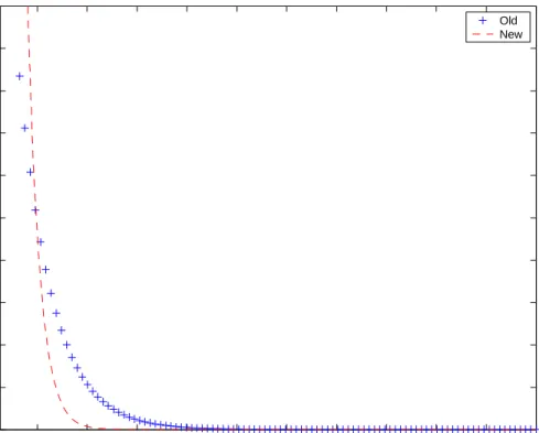
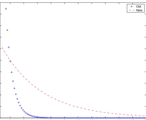
Further insight into this result can be gleaned from the last three figures, which map the
abnormal returns in the chemicals and engineering sectors presented in Table 1 translates to a
less precise signal about managerial effort, increasing the income uncertainty to managers for
any given contract, which is only partly offset by modifying the choice of the optimal contract. By way of contrast, improved precision of the signal in the aerospace sector was more than offset by the changing composition effects of the sector discussed in Tables 9 and 11.
7
Conclusion
Sector differences,firm size, aggregate economic conditions, executive position, and thefirm’s abnormal returns explain almost all variation in managerial compensation. In the three sectors
we examined over the 60 year period, wefind that the higher order moments of the distribution
of abnormal returns have changed significantly. These changes have affected the optimal
con-tract in our model of moral hazard, and as an empirical matter, the nature of the dependence of executive compensation on abnormal returns.
Our results show that losses shareholders would incur from ignoring moral hazard and
paying manager a fixed wage like other administrators has greatly increased. This is because
the abnormal return to the firm from a manager pursuing his own goals in lieu of value
maximization has not changed dramatically, but is now applied to much biggerfirms.
We also find that the value of deviating from the shareholders’ goal of value maximization
has not become more attractive to managers. Our estimates show that the reservation value to take an executive position, to be fully monitored, and to receive the certainty equivalent of a compensation package, have increased at roughly the same rate as GDP, but not more. Preferences to risk have also remained stable in an economic sense. Thus neither changing tastes nor factors outsides our framework can readily explain the increased levels and volatility in managerial compensation.
There are two reasons why we find the welfare of costs of moral hazard have increased. In
two sectors we find that the signal quality shareholders receive about effort has deteriorated. In our empirical framework, this has led to a more dispersed signal, simultaneously raising the average cost of incentivizing managers and subjecting them to more uncertainty in their
incomeflow. In one sector average employment per firm size has increased, and our estimates
show that the interests of managers and firms diverge more in largerfirms. This explains why
the cost of moral hazard has increased in the third sector we investigate.
Our three sectors are quite representative of all sectors, and exhibit trends that have been found in previous studies using other data. Thus thefindings give us confidence to believe that
changes moral hazard induced by technological shifts affecting the distribution of abnormal
returns and the composition of firms are major contributing factors to increased levels and
volatility in managerial compensation.
8
Appendix
In the old sample and the new restricted sample, the data are ordered byn∈{1, .., N}, where
three top executives (imputed using the methods described in our discussion of Table 4), the abnormal return (imputed from the regressions reported in Table 1), the number of employees,
the asset to equity ratio, GDP that year, the bond price in the current year (denotedpn), the
bond price the following year (denotedqn), and sector dummy variables.
Having obtained the Maximum Likelihood estimator for the coefficientsswhich determine
the probability density function for abnormal returns, f2(x), we estimated the remaining
pa-rametersθ≡(ρ, u1, a1, a2, ξ)from orthogonality conditions derived from the participation and
incentive compatibility constraints, along with the score of the likelihood function of the opti-mal contract in a generalized methods of moments procedure, after substituting our estimate forsobtained in the first step. Let the true value ofθ be denoted by θo≡(ρo, uo
1, ao1, ao2, ξo).
Specifically, we constructed a vector of orthogonality conditions from (a vector of three
executives) from the participation constraints of the form
h1n(θ) = exp[−q−n1(ρwen+ξ)]−(a02zn)1/(1−pn) (7)
The distributional assumptions onεn imply
E©exp[−qn−1(ρowen+ξ)] ¯ ¯wn, qn}= exp £ −qn−1(ρown) ¤ (8) Because the participation equation is met with equality under the optimal contract, it follows that
E[h1n(θo)] = 0 (9)
The second vector of orthogonality conditions is based on the incentive compatibility con-straint. Define the vector
h2n(θ, s, ψ) = exp £ −q−n1(ρwen+ξ) ¤∙ f1(xn, s, ψ) f2(xn,θ, s, ψ) − ¡ a01zn ¢1/(pn−1)¸ , (10)
The incentive compatibility constraint is also met with equality under the optimal contract, when the parameters are set to their true values, so this implies:
E[h2n(θo, so, ψo)] = 0. (11) where(so, ψo)are the true values of (s, ψ).
Thefinal set of orthogonality conditions comes from the properties of the optimal contract. According to equation(2) the observed compensation can be written as
e wn=ρ−1qnln ¡ a02zn ¢ + pn (1 +rn) ρ−1ln ∙ 1 +ηn¡a01zn ¢1/(pn−1) −ηn f1(xn, s, ψ) f2(xn,θ, s, ψ) ¸ +εn (12)
whereηn is the unique, strictly positive solution to the following equation in η Z
[η(a01zn)1/(pn−1)−η
f1(xn, s, ψ) f2(xn,θ, s, ψ)
Denoting the density of wen conditional on zn and xn as fθ,s,ψ(wen|zn, xn), we can write the score with respect toθ for the likelihood of observing wen as
h3n(θ, s, ψ) =∇θlnfθ,s,ψ(wen|zn, xn) (14) From the definition of a score
E[h3n(θo, so, ψo)] = 0. (15) Our estimator forθwas found by forming aq×1vector functionhn(θ, s, ψ)fromh1n(θ), h2n(θ, s, ψ) and h3n(θ, s, ψ)and minimizing
" 1 N X n=1 hn(θ, s(N), ψ(N)) #0 AN " 1 N X n=1 hn(θ, s(N), ψ(N)) # (16)
with respect toθ subject to Equation(13) which definesηn,whereAN which is aq×q matrix converging to some constant nonsingular matrixAand the estimators³s(N), ψ(N)´come from thefirst step.
9
Endnotes
1. The surveys by Canice Prendergast (1999), John Abowd and David Kaplan (1999) and Pierre Chiappori and Bernard Salanie (2000) review a growing empirical literature that analyses executive compensation as a tool for regulating managerial decisions that are not directly monitored by shareholders.
2. The first data set, originally constructed by Robert Masson and later extended by Rick
Antle and Abbie Smith, covers the period 1944 to 1978. The second data set, constructed from SEC records and, covers the period 1993 to 2003.
3. For introduction to the vast literature on hidden actions and moral hazard, see the recently published texts of Jean-Jacques Lafont and David Martimont (2002), Bernard Salanie (2005) or Patrick Bolton and Mathias Dewatripont (2005).
4. Several researchers have explored how differences in firms affects managerial
compensa-tion. For example Peter Kostiuk (1990) has analyzed firm size and managerial
compen-sation. Teresa John and Kose John (1993) investigate the capital structure of afirm and
managerial compensation. Evidence provided by Rajeesh Aggaral and Andrew Samwick (1999) shows that the volatility of abnormal returns is inversely related to the
perfor-mance component of executive pay, as the theory of compensating differentials would
predict.
5. Conversely if managers do not hold any market wealth outside their ownfirm and
can-not short sell units of the market portfolio, then compensation should can-not depend on aggregate shocks. Marianne Bertrand and Sendihil Mullainathan (2001) show there is
a positive relationship between strong governance (measured by several dimensions of board composition and managerial tenure) and the ratio of executive pay for
perfor-mance relative to other stochastic factors over which managers have no influence. Their
findings beg the following questions. Are contracts that reward pure luck non-optimal,
or more broadly, evidence that strong governance is a costly factor in production? And
to what extent do such contracts attract managers who can neutralize the effects of pure
luck through portfolio adjustments? While our assumption ascribing pay volatility from aggregate shocks to changes in the manager’s outside wealth rather than his pay is some-what controversial, it reflects our belief that the nature of governance is endogenous to managerial contracting.
6. See Hall and Liebman (1998) and Murphy (1999).
7. This is a standard assumption in principal agent models. See for example Sanford Gross-man and Oliver Hart (1983). In conducting an empirical analysis of executive compen-sation that is explicitly based on a principal agent model, our approach follows the work of John Garen (1994), Joseph Haubrich (1994), and Mary Margiotta and Robert Miller (2000 ), where the derivation of the optimal contract in our model can be found.
8. This equation is derived in Maddala (1983, page 365).
9. See Whitney Newey (1984) for a derivation of this correction.
10. Commenting on the sensitivity of previous results to including measures of firm size in
the analysis, Chiappori and Salanie (2005) that unless heterogeneity between firms is
treated within the analysis, then interpreting the findings and attributing causality is
problematic. Our results add to their discussion by establishing a set of controls that, along with abnormal returns, explain almost all the variation in executive compensation. They imply there is little scope for managerial tenure, or relative performance measures, to explain much variation in compensation.
References
[1] Abowd, John M. and Kaplan, David S. "Executive Compensation: Six Questions
That Need Answering"The Journal of Economic Perspectives,1999 13 (4) pp.145-168.
[2] Aggarwal, Rajesh K. and Samwick, Andrew A. "The Other Side of the Trade-Off:
The Impact of Risk on Executive Compensation"Journal of Political Economy, 1999,
107 (1), pp.65-105.
[3] Antle, Rick and Smith, Abbie. "An Empirical Investigation of the Relative
Perfor-mance Evaluation of Corporate Executives"Journal of Accounting Research, 1986,24
pp.1-39.
[4] Antle, Rick and Smith, Abbie. "Measuring Executive Compensation: Methods and an Application" Journal of Accounting Research, 1985, 23 pp.296-325..
[5] Bertrand, Marianne and Mullainathan, Sendhil."Are CEOS Rewarded for Luck?
The Ones Without Principals Are."The Quarterly Journal of Economics, August 2001,
pp.901-932.
[6] Bertrand, Marianne and Schoar, Antoinette. "Managing with Style: The Effect of
Managers on Firm Policies", The Quarterly Journal of Economics, November, 2003,
CXVII (4) pp.1169-1208.
[7] Bolton, Patrick and Dewatripont, Mathias.Contract Theory, Cambridge, Massa-chusetts: The MIT Press, 2005.
[8] Chiappori, Pierre-André and Salanié, Bernard. "Testing Contract Theory: A
Sur-vey of Some Recent Work",in Advances in Economics and Econometrics - Theory and
Applications, Eighth World Congress, M. Dewatripont, L. Hansen and P. Turnovsky,
ed., Econometric Society Monographs, Cambridge University Press, Cambridge, 2003, pp.115-149.
[9] Garen, John E. "Executive Compensation and Principal-Agent Theory" Journal of
Political Economy, 1994 102 (6), pp.1175-1199.
[10] Gayle, George-Levi and Miller, Robert A. "Identifying Moral Hazrd and Hidden Information in Principal-Agent Models of Executive Compensation", Tepper school of Business, Carnegie Mellon University, August 2005.
[11] Grossman, Sanford and Hart, Oliver. "An Analysis of the Principal-Agent Problem"
Econometrica, 1983, 51 pp. 7-46.
[12] Hall, Brian J. and Liebman, Jeffrey B."Are CEOS Really Paid Like Bureaucrats?"
The Quarterly Journal of Economics, August 1998, CXIII pp. 653-680.
[13] John, Teresa A. and John, Kose. "Top-Management Compensation and Capital Structure"The Journal of Finance, July 1993, 48 (3) pp. 949-974.
[14] Kostiuk, Peter F. "Firm Size and Executive Compensation" The Journal of Human
Resources,1990, 25 (1) pp. 90-105.
[15] Laffont, Jean-Jacques. and Martimont, David. The Theory of Incentives: The
Prinicipal-Agent Model. Princeton University Press, Princeton, 2002
[16] Maddala, G.S. Limited-Dependent and Qualitative Variables in Econometrics, Cam-bridge, England, Cambridge University Press, 1983.
[17] Margiotta, Marry M. and Miller, Robert A. "Managerial Compensation and The
Cost of Moral Hazard"International Economic Review, August 2000, 41 (3) pp.
669-719.
[18] Masson, Robert. "Executive Motivations, Earnings, and Consequent Equity
Perfor-mance"Journal of Political Economy, 1971, 79 pp. 1278-1292.
[19] Murphy, Kevin J. "Executive Compensation", in Handbook of Labor Economics, Volume 3, O. Ashenfelter and D. Card, ed., Elsevier Science B.V., 1999. Chapter 38, pp. 2485-2563.
[20] Newey, Whitney "A Methods of Moments Interpretation of Sequential Estimators"
Economic Letters 14 pp. 201-206 (1984)
[21] Prendergast, Canice. "The Provision of Incentives in Firms" Journal of Economic
Literature XXXVII pp. 7-63 (1999).
[22] Prendergast, Canice. "The Tenuous Trade-off between Risk and Incentives" Journal
of Political Economy, 2002, 110, pp.1071-1102.
[23] Salanié, Bernard. The Economics of Contracts: A Primer, MIT Press, Cambridge, 2005.
[24] Schaefer, Scott"The Dependence of Pay-Perfrmance Sensitivity on the Size of the Firm"
table 1
two measures of abnormal returns in percentage points (standard deviations in parenthesis)
Variables Sector Old New Restricted New All
All 1.883 (31.196) 12.793 (52.091) 11.484 (47.091) Aerospace 7.496 (40.645) 4.321 (30.343)
-Abnormal Returns 1 Chemicals -0.5481 (23.453) -1.071 (40.651) Electronics 4.189 (41.889) 19.948 (57.271) All 1.7E-8 (31.48) 4.17E-7 (53.43) 8.63E-8 (45.903) Aerospace -2.5E-8 (42.24) 8.01E-8 (30.26)
Abnormal Returns 2 Chemicals 3.82E-8 (23.89) 6.51E-8 (48.61) Electronics -1.68E-8 (41.16) 3.84E-7 (59.411)
Table 2
cross-sectional information on sectors all currency in million of $US (2000) (standard deviations in parenthesis)
Variables Sector Old New Restricted New All All 1,243 (2,250) 3,028 (6,830) 4,168 (109,000) Aerospace 1,886 (3,236) 11,500 (14,900) Sales Chemicals 1,246 (2,018) 2,252 (2,091) Electronics 319 (536) 2,469 (6,223) All 589 (1,034) 1,273 (2,863) 1,868 (4,648) Aerospace 391 (680) 3,132 (3,826) Value of Equity Chemicals 677
(1,107) 800 (869) Electronics 159 (365) 1,283 (3,096) All 525 (924) 3,035 (6,550) 9,926 (40,300) Aerospace 726 (130) 10,600 (12,900) Total Assets Chemicals 548
(851) 2,385 (2,380) Electronics 146 (233) 2,551 (6,311) All 27,370 (28,850) 12,208 (26,676) 18,341 (46,960) Aerospace 49,920 (34,335) 58,139 (69,452) Number of Employees Chemicals 23,537
(25,268) 8,351 (9,323) Electronics 10,485 (7,664) 9,195 (18,266) All 1,797 4,150 82,578 Aerospace 355 233 Number of Obsevations Chemicals 1,092 935 Electronics 252 2,092
All 37 151 1,517
Aerospace 5 11
Number of Firms Chemicals 25 40 Electronics 7 100
table 3
cross-section information on total compensation in thousands of $US (2000) (standard deviations in parenthesis)
Rank Sector Old New Restricted New All
All All 528 (1,243) 4,121 (19,283) 2,319 (12,121) CEO All 729 (1,472) 6,109 (24,250) 5,320 (19,369) Non-CEO All 400 (1,026) 2,256 (12,729) 1,562 (9,303) All Aerospace 744 (1,140) 6,407 (20,689) CEO Aerospace 950 (1,292) 11,664 (19,416) Non-CEO Aerospace 624 (695) 1,997 (18,563) All Chemicals 543 (1,348) 2,802 (9,555) CEO Chemicals 718 (1527) 3,673 (7,072) Non-CEO Chemicals 401 (241) 477 (23,390) All Electronics 370 (1,057) 4,501 (22,118) CEO Electronics 457 (1,407) 5,325 (24,576) Non-CEO Electronics 108 (61) 1,635 (18,810)
table 4
cross-section information on components of compensation in thousands of $US (2000) (standard deviations in parenthesis)
Variables Rank Old New Restricted New All All 219 (114) 838 (1,066) 667 (905) Salary and Bonus CEO 261
(115) 1,037 (1,365) 1,127 (1,282) Non-CEO 179 (97) 640 (576) 552 (738) All 79 (338) 2,401 (13,225) 903 (3,753) Value of Options Granted CEO 111
(439 3,402 (18,172) 1.782 (7,169) Non-CEO 51 (198) 1,401 (4,237) 681 (2,106) All 11 (95) 187 (1,633) 152 (936) Value of Restricted
Stock Granted CEO
8 (72) 242 (2,021) 298 (1,464) Non-CEO 13 (112) 133 (1,118) 115 (743) All 5 (134) 785 (14,636) 281 (8,710) Change in Wealth
from Options Held CEO 7 (167) 1,667 (17,078) 1,474 (13,567) Non-CEO 3 (94) -76 (11,706 -18 (6,939) All -3 (439) -40 (5,681) 125 (4,350) Change in Wealth
from Stock Held CEO
0.434 (479) -14 (6,712) 264 (6,791) Non-CEO -7 (398) -64 (4,496) 90 (3,473)
Table 5
parameters of truncated of diligent returns distribution.
(standard errors in parenthesis)
Parameters Sectors Variables Old New
Aerospace
Constant
Asset to Equity Ratio
Number of Employees GDP −1.42 (0.375) −354 (135) −7.08 (1.38) 0.379 (3.14) 4.184 (1.492) 33.57 (49.94) −0.106 (0.135) −8.23 (1.64) σ2 Chemicals Constant
Asset to Equity Ratio
Number of Employees GDP −3.08 (0.097) 77.3 (8.28) −0.352 (0.222) −5.53 (1.15) −4.16 (0.703) −6.92 (7.69) 0.533 (0.559) 1.97 (0.777) Constant −2.07 (0.286) −7.12 (0.426) Asset to Equity Ratio −1.119
(139)
8.926 (13.1) Electronics Number of Employees 0.355
(0.275) 0.877 (0.205) GDP −16.6 (1.93) 5.44 (0.461) Aerospace −0.71 −0.79 ψ Chemicals −0.47 −1.26 Electronics −0.605 −1.6 Aerospace 26.72 (6.00) 20.61 (5.98) p
V ar(xnt|l2nt= 1) Chemicals Standard Deviation 17.42 (3.28)
32.40 (3.96)
Table 6
mean parameter truncated of the shirking returns distribution (standard errors in parenthesis)
Parameters Sector Variables Old New
Aerospace
Constant
Asset to Equity Ratio
Number of Employees GDP −0.051 (0.011) 0.042 (1.71) −0.015 (9.52) −0.056 (11.0) −0.085 (0.001) −0.003 (4.1E−05) 0.019 (3.5E−04) −0.014 (1.9E−04) µ1 Chemicals Constant
Asset to Equity Ratio
Number of Employees GDP −0.015 (0.001) −0.063 (0.074) −0.0428 (0.007) −0.025 (0.002) −0.021 (1.1E−04) −0.071 (0.003) −0.088 (0.002) −0.031 (1.9E−04) Electronics Constant
Asset to Equity Ratio
Number of Employees GDP −2.0E−04 (1.1E−06) −0.025 (4.6E−04) −0.024 (7.8E−04) −0.057 (0.003) −0.008 (3.2E−04) −0.034 (4.5E−04) −0.011 (2.6E−04) −0.017 (6.0E−04) Aerospace −5.5227 (1.47) −8.7553 (1.220) E(xnt|l1nt= 1) Chemicals Mean −3.176 (1.25) −1.7706 (1.22) Electronics −2.1374 (1.56) −2.456 0.23
Table 7
gross losses to firms from shirking in millions of US$ (2000) (standard deviation in parenthesis)
Parameters Industry Old New
Per Year Aerospace 13.751 (29.522) 180.212 (261.294) Present Value 81.065 (177.132) 1,261.484 (1,829.058)
τ1 Per Year Chemicals 33.392 (73.537) 160.038 (240.970) Present Value 200.352 (441.222) 1,120.266 (1,686.79) Per Year Electronics 16.650
(49.182) 230.566 (600.607) Present Value 99.907 (894.492) 1613.962 (4,204.249)
Table 8
nonpecuniary benefits from diligence relative to outside option. (standard errors in parenthesis)
Para-meters Rank Variables Old New
Constant 0.985 (0.048) 3.91 (0.002) Assets −0.475 (0.032) 2.31 (0.009) CEO Employees 1.08 (0.03) 2.8189 (0.011) Aerospace Dummy 2.32 (1.07) 1.06 (0.002) Chemicals Dummy 0.403 (0.066) 1.75 (0.002) α2 Constant 0.838 (0.230) 2.44 (0.005) Assets 1.77 (7.41) 0.605 (0.001) Non-CEO Employees 0.626 (1.96) 2.35 (0.004) Aerospace Dummy 1.29 (11.1) 1.46 (0.011) Chemicals Dummy 0.458 (1.13) −1.42 (0.0003)
Table 9
nonpecuniary benefits from diligence relative to shirking. (standard errors in parenthesis)
Parameters Rank Variables Old New
Constant 3.23 (0.017) 1.85 (0.002) Assets 0.109 (0.012) 2.72 (0.017) CEO Employees 5.06 (0.201) 1.90 (0.058) Aerospace Dummy 10.224 (4.17) 13.123 (0.062) Chemicals Dummy 8.0 (0.309) 9.53 (0.049) α2/α1 constant 3.08 (1.73) 3.02 (0.011) Assets 13.0 (4.07) 7.39 (0.125) Non-CEO Employees 3.06 (1.96) 2.35 (0.041) Aerospace Dummy 4.47 (9.22) 8.39 (0.123) Chemicals dummy 2.35 (1.86) 8.04 (0.159)
Table 10
Absolute risk aversion (standard error in parenthesis)
parameters Old New
ρ 0.5189 (3.0E−07) 0.501 (1.2E−09) ξ 0.008 (1.3E−10) 0.101 (3.8E−10) R2 0.856 0.9578 Table 11
nonpecuniary benefits of shirking in thousands of US$ (2000) (standard deviation in parenthesis)
Parameters Industry Rank Old New
Aerospace CEO Non CEO 279 (76) 160 (50) 397 (420) 340 (786) τ2 Chemicals CEO Non CEO 117 (56) 113 (35) 48 78) 88 (98) Electronics CEO Non CEO 240 (56) 130 (35) 220 78) 240 (98)
Table 12
welfare cost of moral hazard in thousands of $US (2000) (standard deviation in parenthesis)
Parameters Industry Rank Old New
Aerospace CEO Non CEO 500 (1,316) 330 (1,413) 10,350 (15,473) 1,280 (10,501) τ3 Chemicals CEO Non CEO 490 (1,437) 299 (206) 2,973 (5,087) 301 (1,678) Electronics CEO Non CEO 278 (1,257) 67 (188) 4,873 (17,285) 1,206 (11,159)
0 2 4 6 8 10 12 14 16 18 20 0 0.2 0.4 0.6 0.8 1 1.2 1.4 1.6 1.8 2 x g (x ) Old New
0 2 4 6 8 10 12 14 16 18 20 0 0.2 0.4 0.6 0.8 1 1.2 1.4 1.6 1.8 2 x g (x ) Old New
-5 0 5 10 15 20 0 0.2 0.4 0.6 0.8 1 1.2 1.4 x g (x ) Old New