Measuring volatility with the realized range
∗
Martin Martens
† Econometric Institute Erasmus University RotterdamDick van Dijk
‡ Econometric Institute Erasmus University RotterdamEconometric Institute Report EI 2006-10
February 2006
Abstract
Realized variance, being the summation of squared intra-day returns, has quickly gained popularity as a measure of daily volatility. Following Parkinson (1980) we replace each squared intra-day return by the high-low range for that period to create a novel and more efficient estimator called the realized range. In addition we suggest a bias-correction procedure to account for the effects of microstructure frictions based upon scaling the realized range with the average level of the daily range. Simulation experiments demonstrate that for plausible levels of non-trading and bid-ask bounce the realized range has a lower mean squared error than the realized variance, including variants thereof that are robust to microstructure noise. Empirical analysis of the S&P500 index-futures and the S&P100 constituents confirm the potential of the realized range.
Keywords: Realized volatility; high-low range; high-frequency data; market microstructure noise, bias-correction.
JEL Classification: C14, C15, C53.
∗We thank Peter Hansen, participants at the International Conference on Finance in Copen-hagen (September 2-4, 2005), the special issue guest editors Herman van Dijk and Philip Hans Franses, and two anonymous referees for useful comments and suggestions. Any remaining errors are ours.
†Econometric Institute, Erasmus University Rotterdam, P.O. Box 1738, NL-3000 DR Rot-terdam, The Netherlands, Phone: +31 10 408 1285, Fax: +31 10 408 9162, E-mail: [email protected]
‡Econometric Institute, Erasmus University Rotterdam, P.O. Box 1738, NL-3000 DR Rot-terdam, The Netherlands, Phone: +31 10 408 1263, Fax: +31 10 408 9162, E-mail: [email protected](corresponding author)
1
Introduction
Measuring and forecasting volatility of financial asset returns is important for portfo-lio management, risk management and option pricing. By now it is well established that volatility is both time-varying and, to a certain extent, predictable. An im-portant issue is how to measure ex-post volatility, which is necessary for proper evaluation of competing volatility forecasts, among other purposes. Recently much research has been devoted to the use of high-frequency data for measuring volatil-ity. In particular, the sum of squared intra-day returns, called realized variance, is rapidly gaining popularity for estimating daily volatility. In theory, the realized vari-ance is an unbiased and highly efficient estimator, as illustrated in Andersen et al. (2001b), and converges to the true underlying integrated variance when the length of the intra-day intervals goes to zero, see Barndorff-Nielsen and Shephard (2002). In practice, market microstructure effects such as bid-ask bounce pose limitations to the choice of sampling frequency. Returns at very high frequencies are distorted such that the realized variance becomes biased and inconsistent, see Bandi and Rus-sell (2005a,b), A¨ıt-Sahalia et al. (2005), and Hansen and Lunde (2006b). Popular choices in empirical applications are the five- and thirty-minute intervals, which are believed to strike a balance between the increasing accuracy of higher frequencies and the adverse effects of market microstructure frictions, see e.g. Andersen and Bollerslev (1998), Andersen et al. (2001a), Andersen et al. (2003), and Fleming et al. (2003).
An alternative way of measuring volatility is based on the difference between the maximum and minimum prices observed during a certain period. Parkinson (1980) shows that the daily (log) high-low range, properly scaled, not only is an unbiased estimator of daily volatility but is five times more efficient than the squared daily close-to-close return. Correspondingly, Andersen and Bollerslev (1998) and Brandt and Diebold (2006) find that the efficiency of the daily high-low range is between that of the realized variance computed using 3-hour and 6-hour returns.
the relative efficiency of the high-low range applies to any interval, in particular also to the intra-day intervals employed by the realized variance. That is, in theory, for each intra-day interval the high-low range is a more efficient volatility estimator than the squared return over that interval. We therefore suggest to measure daily volatility by the sum of high-low ranges for intra-day intervals. The resulting es-timator, which we dub ‘realized range’, should be more efficient than the realized variance based on the same sampling frequency. Indeed, in concurrent independent work, Christensen and Podolskij (2005) derive the theoretical properties of the real-ized range, similar to Barndorff-Nielsen and Shephard (2002) for realreal-ized variance. In an ideal world (continuous trading, no market frictions) the realized range is five times more efficient than the corresponding realized variance, and converges to the integrated variance at the same rate. At the same time, in such an ideal world there seems to be no need to consider the realized range, as the true daily volatility can be approximated arbitrarily closely by the realized variance using higher and higher frequencies. However, it is often claimed that the daily range is more robust against the effects of market microstructure noise than the realized variance, see Alizadeh et al. (2002) and Brandt and Diebold (2006), among others. Obviously, the realized range will be affected more heavily by microstructure noise as each of the intra-day ranges is contaminated. Nevertheless, in realistic settings it is an open question as to whether the realized variance or the realized range renders a superior measure of daily volatility. In this paper we attempt to shed light on this question.
Our approach is based upon Monte Carlo simulation and an empirical analysis for S&P500 index-futures and the individual stocks in the S&P100 index. The simulation experiments reveal that both realized range and realized variance are upward biased in the presence of bid-ask bounce. We find that in fact the realized range is affected more than the realized variance at the same sampling frequency. Infrequent trading induces a downward bias in the realized range, while it does not affect the realized variance. In case the price path is not observed continuously the observed minimum and maximum price over- and underestimate the true minimum and maximum, respectively, such that the observed range underestimates the true
range.
We consider a bias-adjustment procedure for the realized range estimator, which involves scaling the realized range with the ratio of the average level of the daily range and the average level of the realized range. This is based upon the idea that the daily range is (almost) not contaminated by microstructure noise and thus provides a good indication of the true level of volatility. In the simulation experiments, we find that the scaled realized range is more efficient than the (scaled) realized variance estimator based on returns sampled at considerably higher frequencies. Comparing the scaled realized range with popular corrections of the realized variance for microstructure noise, we find that it outperforms kernel-based estimators, as considered by Barndorff-Nielsen et al. (2004) and Hansen and Lunde (2005, 2006b), and is competitive to the two time-scales estimator of Zhang et al. (2005).
The empirical analysis confirms that for both measuring and forecasting volatility the (scaled) realized range can compete with and often improves upon realized vari-ance estimators at popular sampling frequencies, including the versions that correct for microstructure noise. This is slightly more so for more actively traded stocks.
The remainder of this paper is organized as follows. Section 2 defines the realized range, including the suggested bias-adjustment procedure to counter the adverse effects of market microstructure noise. Section 3 describes the design and results of the simulation experiments that illustrate the properties of the realized range in the presence of market microstructure frictions. Section 4 presents the empirical results for the S&P500 index-futures, both concerning basic properties of the realized range and a comparison between realized range and realized variance. Section 5 extends the comparison to the constituents of the S&P100 index. Finally Section 6 concludes.
2
The realized range estimator
Let the security price Pt at time t follow the geometric Brownian motion
where µ denotes the drift term, σ is the constant volatility parameter and Bt is a
standard Brownian motion. By Ito’s lemma, the log price process logPt follows a
Brownian motion with driftµ∗ =µ−σ2/2 and volatility σ. For ease of notation we
normalize the daily interval to unity. Then for the i-th interval of length ∆ on day
t, for i= 1,2, . . . , I with I = 1/∆ assumed to be integer, we observe the last price in that interval Ct,i = Pt−1+i∆, the high price Ht,i = sup(i−1)∆<j<i∆Pt−1+j and the
low price Lt,i = inf(i−1)∆<j<i∆Pt−1+j. If the drift µ∗ is equal to zero, an unbiased
estimator of the variance during interval i, σ2∆, is the squared return,
rt2−1+i∆,∆= (logCt,i−logCt,i−1)2, (2)
which has variance equal to 2σ4∆2. Parkinson (1980) proposes the scaled high-low
range estimator for the variance,
(logHt,i−logLt,i)2
4 log 2 , (3)
which is also unbiased if µ∗ = 0, but has variance (9ξ(3)/((4 log 2)2)−1)σ4∆2 ≈
0.407σ4∆2, where ξ(3) =P∞
k=11/k3 is Riemann’s zeta function. Hence the variance
(and the mean squared error) of the squared return (2) is about five times larger than that of the high-low estimator (3).
If we are interested in estimating the daily variance, we can aggregate either squared intra-day returns to obtain the so-called realized variance RV∆
t or high-low
ranges for intra-day intervals to obtain the realized range RR∆
t : RVt∆= I X i=1 rt2−1+i∆,∆, (4) RRt∆= 1 4 log 2 I X i=1
(logHt,i−logLt,i)2. (5)
If prices follow the continuous geometric Brownian motion with driftµ=σ2/2 and
constant volatility σ as specified in (1), it is straightforward to show that both
RR∆t and RVt∆ are unbiased and consistent estimators of the daily variance σ2.
In addition, the relative efficiency result stated before for the squared daily return versus the daily high-low range continues to hold for RV∆
t and RRt∆: the variance
A few remarks concerning the (realized) range estimators are in order. First, Garman and Klass (1980) suggest to further improve efficiency by utilizing the open and close prices in addition to the high and low prices. Assuming that the first price in thei-th interval, Ot,i, is identical to the last price in the (i−1)-st interval,Ct,i−1,
their minimum variance unbiased estimator for the volatility during thei-th interval of day t is given by
0.511(logHt,i−logLt,i)2−0.383(logCt,i−logCt,i−1)2
−0.019[(logCt,i−logCt,i−1)(logHt,i+ logLt,i −2 logCt,i−1)
−2(logHt,i −logCt,i−1)(logLt,i−logCt,i−1)], (6)
which is theoretically 7.4 times more efficient than the squared return in (2). They also propose a “practical” estimator achieving virtually the same efficiency, which is simply a linear combination of the high-low range and the squared close-to-close return:
0.5(logHt,i−logLt,i)2−(2 log 2−1)(logCt,i−logCt,i−1)2. (7)
In the context of the daily range, Brown (1990) and Alizadeh et al. (2002) argue against the use of open and close prices, based on the fact that these are heavily contaminated by market microstructure effects. This argument applies only to the open and close prices of a trading day, and as such it does not carry over to the context of the realized range, where open and close prices of the intra-day intervals are ‘regular’ prices observed throughout the day. Indeed, we included realized range estimators based on (6) and (7) in the simulation experiments discussed in the next section, and found that they further improve the efficiency relative toRR∆
t defined in
(5). Detailed results are not reported here for space considerations, but are available upon request.
Second, the assumption of zero drift, µ∗ = µ−σ2/2 = 0 in (1), is crucial for
(1991) were the first to relax this assumption and suggested the estimator (logHt,i−logCt,i−1)(logHt,i −logCt,i)
+ (logLt,i−logCt,i−1)(logLt,i−logCt,i), (8)
which is independent of the driftµand is only slightly less efficient than the Garman-Klass estimator in (6) in case µ=σ2/2. Subsequently, Kunitomo (1992) and Yang
and Zhang (2000) put forward alternative estimators that allow for non-zero drift, essentially by considering a transformed price process to eliminate the drift.1
Finally, and most important for our purposes, Christensen and Podolskij (2005) establish consistency of the realized range estimator RR∆
t as defined in (5) for the
integrated variance under the assumption that the log price follows a continuous sample path martingale, that is
logPt= logP0+ Z t 0 µsds+ Z t 0 σs−dBs, for 0≤t <∞,
where the instantaneous mean µ={µt}t∈[0,∞) is a locally bounded predictable
pro-cess, the spot volatility σ = {σt}t∈[0,∞) is a c`adl`ag process, Bs again is a standard
Brownian motion, and σs− = limt↑sσt. Under the additional assumptions that µ
is continuous and σ is everywhere invertible, the asymptotic distribution of RR∆
t
is shown to be mixed normal, with σ governing the mixture. This result is impor-tant for two reasons. First, it allows for general specifications of the drift µ, which is possible thanks to the fact that the mean component vanishes sufficiently fast as ∆→0. Second, the range estimator traditionally has been analyzed under the strict assumption that volatility is constant (at least within a trading day). The results of Christensen and Podolskij (2005) demonstrate that the realized range estimator remains consistent in the presence of stochastic volatility. The conditions on σ are in fact rather weak, and allow for models with leverage, long-memory, jumps and diurnal effects.
1Bali and Weinbaum (2005) provide a thorough comparison of all the different daily range
2.1
Bias-correcting the realized range
The effects of microstructure noise such as bid-ask bounce on realized variance esti-mators has been studied intensively, see Barndorff-Nielsen et al. (2004), Bandi and Russell (2005a,b), Zhang et al. (2005), and Hansen and Lunde (2006b), among oth-ers. As mentioned before, the realized range may also be expected to suffer from market microstructure effects. In case prices are observed continuously, the high price is likely to be an ask while the low price is likely to be a bid such that the observed range overestimates the true range by exactly the spread. As this will be the case for each intra-day interval, this may cause a substantial upward bias in the realized range for high sampling frequencies. One may attempt to correct for this bias by subtracting the spread from each intra-day range, as suggested by Brandt and Diebold (2006) in the context of the daily high-low range estimator. However, in practice prices are not observed continuously such that the high price may actually be a bid with a certain probability that depends on the trading intensity, complicat-ing this bias-adjustment. In addition, as mentioned before infrequent tradcomplicat-ing itself induces a downward bias in the realized range, as the observed minimum and maxi-mum price over- and underestimate the true minimaxi-mum and maximaxi-mum, respectively. Two procedures have been suggested for correcting the downward bias in the range due to infrequent trading. First, Rogers and Satchell (1991) derive expressions for the expected difference between the observed high and low prices and their true but unobserved counterparts. For the i-th interval during day t, the (log of the) observed high and low price, Ht,i and Lt,i are equal to
logHt,i = logHt,i∗ −δH and logLt,i = logL∗t,i+δL,
whereH∗
t,i and L∗t,i are the true maximum and minimum prices, respectively. Under
the assumption of equidistant prices, Rogers and Satchell (1991) show thatE[δH] =
E[δL] = aσ/√Ni with a =
√
2π(14 − (√2− 1)/6], and E[δ2
H] = E[δ2L] = bσ2/Ni
withb = (1 + (3π/4))/12, where Ni is the number of prices observed during thei-th
of the high-low range estimator given in (3) is the positive root of the equation ˆ σ2 = (b+a 2) 2Nilog 2 ˆ
σ2 +a(log√Ht,i−logLt,i)
Nilog 2
ˆ
σ+ (logHt,i−logLt,i)
2
4 log 2 . (9)
Second, Christensen and Podolskij (2005) argue that the downward bias in the (realized) range is caused by the fact that the scaling factor 4 log 2 in (3) is not appropriate in the presence of infrequent trading. This factor derived by Parkinson (1980) is equal to the second moment of the range of a standard Brownian motion
Bt, that is E[s2B] = 4 log 2, where
sB = sup
0≤s,t≤1
(Bt−Bs). (10)
Christensen and Podolskij (2005) suggest to replace this factor by the expected value of the squared range of a Brownian motion that is observed Ni times, the number
of observations during the i-th intra-day interval. In case of equidistant prices, for example, this boils down to
E max 1≤k,l≤Ni (Bl/Ni −Bk/Ni) 2 .
Unreported results from the simulation experiments in the next section show that both bias-correction procedures work adequately, in that they remove the downward bias in the realized range estimators due to infrequent trading to a large extent, even for the highest frequencies. The Christensen-Podolskij procedure achieves a slightly lower RMSE than the Rogers-Satchell procedure. A limitation of both correction procedures is, however, that they cannot cope with the upward bias induced by bid-ask bounce. Hence, we suggest an alternative bias-correction procedure by scaling the realized range with the ratio of the average level of the daily range and the average level of the realized range over the q previous trading days. That is, the scaled realized range is defined as
RR∆S,t = Pq l=1RRt−l Pq l=1RR∆t−l RR∆t , (11)
where RRt ≡ RR1t denotes the daily range. This is based upon the idea that the
a good indication of the true level of volatility. An important choice to be made when implementing this bias-adjustment is of course the number of trading days q
used to compute the scaling factor. If the trading intensity and the spread do not change for the asset under consideration, q may be set as large as possible in order to gain accuracy. Of course, in practice both features tend to vary over time, which suggests that only the recent price history should be used and q should not be set too large. We return to this issue below.
We close this section by discussing several alternatives for bias-correcting the
RV∆
t estimator that have been put forward recently and that will be included in the
subsequent analysis. First, the scaling procedure suggested for the realized range also can be applied to the realized variance estimator. That is, the scaled realized variance, RV∆
S,t, may be obtained from (11) by replacing RR with RV. See Hansen
and Lunde (2005) for a theoretical justification of this scaling estimator.
Second, the effect of bid-ask bounce (and presumably other types of microstruc-ture noise) can be removed by adding autocovariances to the realized variance. In particular, we consider the RV∆
AC1,t estimator, which incorporates the first-order
autocovariance, RVAC∆1,t = I X i=1 r2t−1+i∆,∆+ 2 I X i=2 rt−1+i∆,∆rt−1+(i−1)∆,∆. (12)
We refer to Barndorff-Nielsen et al. (2004) and Hansen and Lunde (2005, 2006b) for an in-depth analysis of the properties of this realized variance estimator.
Third, Zhang et al. (2005) develop the so-called two time-scales (TTS) estimator, which combines realized variance estimators obtained from returns sampled at two different frequencies. In particular, the realized variance estimator obtained using a certain (low) frequency is corrected for bias due to microstructure noise using the realized variance obtained with the highest available sampling frequency. The essential argument is that the low-frequency estimator renders a biased estimate of the true integrated variance with the bias being a function of the variance of the noise in the return processes. The realized variance estimator using the highest possible frequency consistently estimates this noise variance and can therefore be used to
reduce and potentially even eliminate the bias of the low-frequency estimator. In addition, subsampling is used to reduce the variance of the low-frequency realized variance estimator as follows. Assume that we observe N + 1 equidistant prices during the trading day, whereN is an integer multiple ofI, the number of intra-day intervals corresponding to a particular sampling frequency. In that case, the grid of intervals of length ∆ = 1/I can be laid over the trading day in N/I different ways. For example, in case prices observed once every minute, for the realized variance based on the five-minute sampling frequency rather than starting with the interval 9:30-9:35 one could also start with 9:31-9:35, 9:32-9:37, 9:33-9:38 or 9:34-9:39. In this way five ‘subsamples’ are created and each of these can be used to compute the realized variance. The final realized variance is then taken to be the average across subsamples. A practical problem with this procedure is how to treat the loose ends at the start and the end of the trading session. Here we omit these and proportionally inflate the realized variances for the missing part of the trading day. Based on the above, the two time-scales estimator RV∆
T T S,t is obtained as RVT T S,t∆ = N N −I RVSubs,t∆ − I NRVM ax,t , (13) whereRV∆
Subs,t is the subsampling estimator using returns over intervals of length ∆
with I = (I−1) +I/N being the average number of intraday return observations used by each of the realized variance estimators used in the subsampling process, and
RVM ax,t is the realized variance based on the highest possible sampling frequency
using all N return observations.
3
Simulation
We simulate prices for 24-hour days, assuming that trading can occur round the clock. For each day t, the initial price is set equal to 1, and subsequent log prices are simulated using
where J is the number of prices per day. To approximate the ideal situation with continuous trading and no market frictions we simulate 100 prices per second, such that J = 8,640,000 as there are 86,400 seconds in a 24-hour day. The shocks εt+j/J
are independent and normally distributed with mean zero and variance σ2/(D·J),
where total annualized standard deviation σ of the log price process is set equal to 0.21 (21%), and D is the number of trading days in a year, which we set equal to 250. We simulate prices for 5000 trading days in all experiments reported below.
To illustrate the promise of realized range as a measure of (daily) volatility we compute both the realized range and the realized variance for the prices simulated in the ideal world as described above. To do so we divide the trading day into x -minute intervals, which is called the x-minute frequency. For example when x = 1 we divide the 24-hour day into 1440 1-minute intervals. For the realized variance the squared 1-minute returns are summed to obtain the realized variance at that frequency. For the realized range the high and low are computed per 1-minute interval and the resulting 1-minute ranges are summed to obtain the realized range for the day. We also consider the scaled versions of the realized range and the realized variance computed according to (11). In subsequent experiments with non-trading and bid-ask bounce, the characteristics of these microstructure frictions are identical for all trading days, such that we can use a large number of trading days q
to compute the scaling factor. We therefore set we setq = 5000 to fully explore the possibilities of the scaling bias-adjustment procedure. The sensitivity of the results with respect to the value ofqis discussed in more detail below. Finally, the RV∆
AC1,t
kernel-based estimator and the two time-scales estimator RV∆
T T S,t are included. For
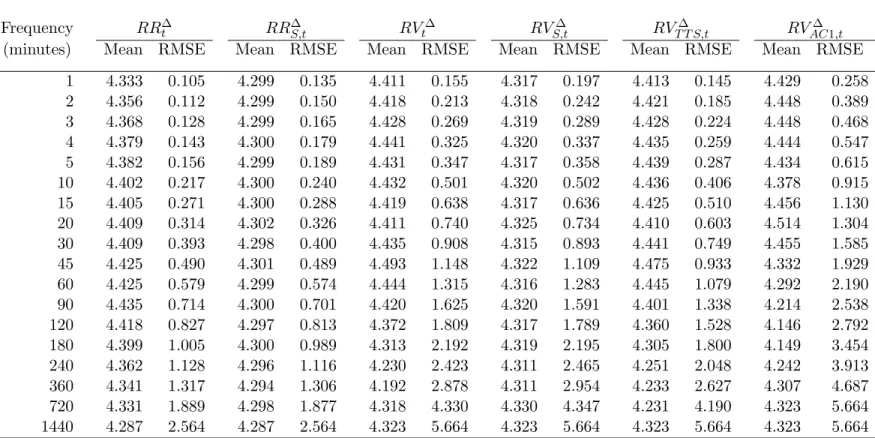
the latter we use all observed prices to compute the realized variance at the highest possible frequency to obtain an accurate estimate of variance of the measurement noise, and implement the subsampling estimator by shifting the intra-day intervals ten seconds at a time. For each selected frequency we compute the mean and Root Mean Squared Error (RMSE) for the various volatility estimators, taken over 5000 simulated trading days. The results are presented in Table 1.
-For x = 1440 minutes (the final row in the table) the realized range equals the daily high-low range and the realized variance equals the daily squared return. As expected the RMSE of the range is substantially lower at 2.564 than that for the daily squared return at 5.664, reflecting the fact that the daily range is five times more efficient than the daily squared return. Akin to the findings of Andersen and Bollerslev (1998) and Brandt and Diebold (2006) the realized variance requires the 4-hour (240 minutes) frequency to achieve a similar RMSE as the daily range. Obviously in this case the RMSE of the realized range is always substantially lower than that of the realized variance at the same frequency. We also observe that the RMSE of the TTS estimator is lower than the RMSE of the corresponding realized variance estimator, because of the reduction in variance due to the subsampling used. This is not sufficient though to achieve the same efficiency as the realized range estimator. Finally, in the absence of microstructure noise, the RMSE of the
RV∆
AC1,t estimator is about 1.7 times the RMSE of the standard realized variance,
cf. the theoretical results of Hansen and Lunde (2005, 2006b).
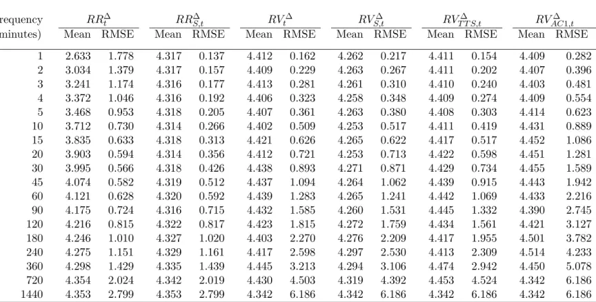
From Table 1 it appears that the realized range is slightly downward biased for the highest frequencies (the true variance is 4.41). This is inherent to the nature of the high-low range: In case the price path is not observed continuously (in our case we observe ‘only’ 6000 prices per minute) the observed minimum and maximum over- and underestimate the true high and low prices, respectively, such that the observed range underestimates the true range. To investigate this problem in more detail Table 2 shows the results when infrequent trading occurs, such that the price is observed on average only everyτ = 10 seconds. That is, given the simulated paths underlying Table 1, the probability to observe the price is equal toπ = 1/(100τ).
insert Table 2 about here
-The results for the realized range show that the RMSE first declines when in-creasing the sampling frequency up to the 30-minute frequency. Then it increases again for higher frequencies because the increase in the bias due to non-trading (and hence underestimating the range for each intra-day interval) then outweighs the
re-duction in the standard deviation of the estimates. The different realized variance estimators are not affected by infrequent trading, except for a slight increase in the (standard deviation and thus in) RMSE. As a result at the 30-minute frequency, for example, the realized range still is a more accurate volatility measure than the corresponding realized variance, but at the 5-minute frequency the realized variance has a substantially lower RMSE than the realized range. Of course the exact fre-quency at which one estimator improves over the other will depend on the trading intensity. For example when observing a price on average every second the realized range improves over the realized variance up to the 5-minute frequency. Unreported results using the bias-correction procedures of Rogers and Satchell (1991) and Chris-tensen and Podolskij (2005), which are explicitly designed for handling the effects of infrequent trading, shows that both procedures work satisfactorily, in the sense that they largely remove the bias in the realized range estimators, even for the highest frequencies. The results for RR∆
S,t in Table 2 demonstrates that scaling the realized
range does not eliminate the bias completely, which is due to the fact that the daily range also is somewhat biased downward due to the infrequent trading. In terms of RMSE, the scaling procedure is slightly better than the Rogers-Satchell procedure, and only slightly worse than the Christensen-Podolskij procedure. For example, at the 5-minute frequency the RMSE of RR∆
S,t is equal to 0.205, compared to 0.229
and 0.187 for the bias-corrected realized range estimators based upon (9) and (10), respectively.
As noted in the previous section, the number of trading days q used to compute the scaling factor for RR∆
S,t is a crucial choice to be made. If the trading intensity
and the spread are constant over time,q may be set large in order to gain accuracy. On the other hand, when the magnitude of these microstructure frictions varies over time, only the recent price history should be used and q should be set fairly small. Figure 1 shows the RMSE of the scaled realized range for the experiment with infrequent trading as a function of q, with the rightmost point of each line showing the RMSE for q = 5000 as given in Table 2. The RMSE monotonically declines as
more or less stabilizes. Also note that the reduction in RMSE due to increasing qis largest for higher sampling frequencies.
insert Figure 1 about here
-Next, we consider the effects of bid-ask bounce. For this purpose we assume that transactions take place either at the ask price or at the bid price, which are equal to the true price plus and minus half the spread, respectively. Hence, if a transaction occurs att+j/J, the actually observed price P∗
t+j/J is equal toPt+j/J+s/2 (ask) or
Pt+j/J−s/2 (bid), wheresis the bid-ask spread andPt+j/J is the true price obtained
from (14). As in Brandt and Diebold (2006), we set s = 0.0005 (or 0.05% of the starting price of 1) and assume that bid and ask prices occur equally likely.
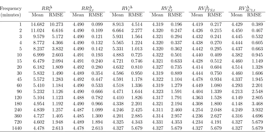
The results in Table 3 show that as expected both realized range and realized variance suffer upward bias, which gets worse as the sampling frequency increases. The bias in the realized range is caused by the fact that in the limit the observed range will overestimate the true range by exactly the spread, as the maximum price will be an ask and the minimum price will be a bid. The realized variance is biased upwards because half of the times (when the return is computed from bid to ask or from ask to bid) the squared bid-ask spread is included. The realized range is affected more by the bid-ask bounce than the realized variance, when comparing them at the same sampling frequency. In this particular parameter setting the realized range outperforms the realized variance up to the 1-hour (60-minute) frequency. For higher sampling frequencies the RMSE of the realized variance is lower. Scaling the realized range works remarkably well, in the sense that the bias is removed completely and the RMSE values are brought back to the original level observed for RR∆
t in the
ideal case without bid-ask bounce shown in Table 1, or even slightly below. The unreported results for the bias-correction procedures of Rogers and Satchell (1991) and Christensen and Podolskij (2005) show that logically they completely fail to correct for the bid-ask bounce effects. Scaling the realized variance also removes a large part of the bias, but at frequencies higher than 60 minutes, say, the RSME remains substantially higher than the RMSE ofRV∆
RV∆
T T S,t and RVAC∆1,t are robust to the presence of bid-ask bounce. Note that the
scaled realized range outperforms the TTS estimator (and therefore the kernel-based estimator as well) at all frequencies considered.
insert Table 3 about here
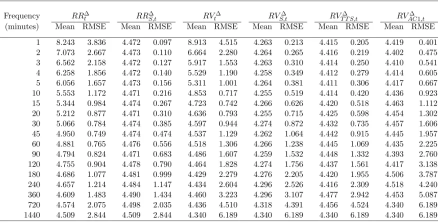
-Finally, we consider the realistic situation where both bid-ask bounce and in-frequent trading are present, combining the specifications for these two frictions as discussed before. Results of this experiment are shown in Table 4. The realized range still suffers from an upward bias, but of a considerably smaller magnitude than in the case of bid-ask bounce only due to the off-setting negative bias induced by infrequent trading. As a result, the realized range now has a lower RMSE than the realized variance up to the 30-minute frequency, as well as at the 1-minute fre-quency. In addition the overall minimum RMSE is obtained at 0.749 for the realized range at the 45-minute frequency. For the realized variance the optimal frequency is the 10-minute frequency for which the RMSE is 0.717, hence only slightly smaller than that for the optimal realized range. Also here we find that scaling the realized range works adequately in removing the bias and bringing the RMSE of the RR∆
S,t
estimator down to the levels originally observed in the case of no market microstruc-ture frictions. Finally, again we observe that the two time-scales estimator and the kernel-based estimator remain unbiased, but their RMSEs are higher than those of the scaled realized range.
insert Table 4 about here
-Concluding, the simulation experiments quite convincingly demonstrate the po-tential of the realized range as a measure of volatility. In case of continuous trading and no market frictions it always improves upon the popular realized variance when using the same sampling frequency. In reality trading is discontinuous and observed prices are bid and ask prices. In that case scaling the realized range with the average (relative) level of the daily range is an effective procedure to remove the induced bias and restore the efficiency of the realized range. Of course these results are obtained
assuming a specific price process that may affect the results. In particular, we have assumed that the microstructure noise is temporally independent and independent from the true price process. As discussed in Hansen and Lunde (2006b), there is substantial empirical evidence against both these assumptions at ultra-high frequen-cies. Further investigation of the properties of the realized range estimator under more general specifications of the noise process is therefore warranted. As such it will also be interesting to look at its performance for actual market data in Sections 4 and 5 below.
4
S&P500 index futures
The S&P500 index-futures contract is the largest equity futures contract in the world. It is trading virtually round the clock, with floor trading on the Chicago Mercantile Exchange (CME) from 9:30 to 16:15 Eastern Standard Time (EST), and electronic trading on GLOBEX almost 24 hours a day apart from Friday evening to Sunday evening. Our sample contains transaction prices and bid and ask quotes running from 4 January 1999 to 23 February 2004. The S&P500 futures contract has maturities in March, June, September and December. We always use the most liquid contract (usually until 1 week before the maturity of that contract) and make sure that when changing from one contract to the next, we never compute returns based on prices from two different contracts. For the 1289 days in the sample period this results in on average 3,223 transaction prices during floor trading from 9:30 to 16:15 EST and 1,802 transactions during the remainder of the day with a substantial number taking place in the run-up to the opening of the New York Stock Exchange (NYSE) at 9:30 EST. The spread is relatively small but varies considerably over time. For example, for the September 2001 contract the average spread (based on bid and ask quotes with the same time stamp to the nearest second) is 0.443 index-points on an average futures price of 1190 (0.037%), whereas for the December 2003 contract it is 0.220 on an average price of 1039 (0.018%). Hence such a liquid contract does not exactly reflect the ideal situation with continuous trading and no market frictions,
but it is not far off either. In Section 5 we will repeat some of the analysis below for the S&P100 index constituents that provide much more noisy data. The variation in the average spread implies that the ratio of the average level of the daily range relative to the average level of the realized range changes over time. For this reason we compute the scaling factor for RR∆
S,t in (11) using the previous q = 66 trading
days or approximately three months.
4.1
Characteristics of realized range
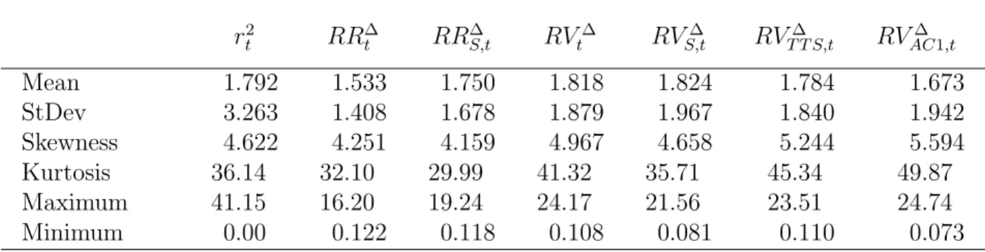
Initially we follow Andersen, Bollerslev, Diebold and Ebens (2001) (henceforth ABDE) by documenting the characteristics of the realized range defined in (5) mea-sured using five-minute intervals from 9:30-16:15 EST (as in ABDE) and 15-minute intervals from 16:15 to 9:30 EST. For comparison we also include the properties of a number of other estimators. Table 5 shows selected sample statistics for the squared daily returns, r2
t, the realized range (RR∆t ), the realized variance (RVt∆), the scaled
realized range and realized variance (RR∆S,tandRVS,t∆), the two time-scales estimator (RV∆
T T S,t) and the kernel-based estimator (RVAC∆1,t).
insert Table 5 about here
-The mean daily squared (close-to-close) return is 1.792 implying an annualized standard deviation for the S&P500 index of around 21.4%. The mean realized vari-ance is close to this (1.818), whereas as expected the realized range has a lower average at 1.533. Hence it seems that bid-ask bounce is not a crucial issue at the se-lected sampling frequency, whereas not observing a continuous path of prices causes a downward bias in the realized range. This problem will obviously increase for higher frequencies. We return to this point below when considering results for other sampling frequencies. Here we note that scaling the realized range with the ratio of the average level of the daily range for the previousq= 66 days, as in (11), increases the average to 1.750, more in line with the realized variance.
Both the realized variance and the realized range are right-skewed and leptokur-tic, although less so for the realized range than for the realized variance. The
stan-dard deviation of the daily squared returns is 3.263, substantially higher than the standard deviation of the realized variance at 1.879. This is in line with the notion that both measures are unbiased but realized volatility is less noisy. The standard deviation of the TTS estimator is only slightly lower at 1.840, while that of the kernel-basedRV∆
AC1,t estimator is higher at 1.942. This also suggests that the effects
of microstructure noise are limited for the S&P500 index-futures contract. Finally, we observe that the realized range is even less noisy with a standard deviation of 1.408. Even after adjusting for the bias the standard deviation remains below that of the realized variance at 1.678, underlining the potential of the realized range estimator.
ABDE report that daily returns standardized with the realized standard devia-tions are approximately Gaussian for the 30 Dow Jones stocks. Table 6 reports the corresponding results for the realized range. The results in the first column for the daily returns show that normality is rejected at conventional significance levels. For the daily returns standardized with the square root of the (scaled) realized range, however, the sample kurtosis is reduced to 2.814 (2.800) from 4.310 for the raw re-turns. Note that the Jarque-Bera test statistic is asymptotically χ2(2), with a 5%
critical value of 5.99 (1%: 9.21). Hence for the daily returns standardized with the (square root of the) (scaled) realized range the null hypothesis of normality cannot be rejected. In contrast, for the daily S&P500 returns standardized with the (scaled) realized standard deviation the null of normality is rejected at the 5% significance level.
insert Table 6 about here
-We examine the effect of the sampling frequency on the properties of the realized range by varying the length of the intra-day intervals. For the floor trading period be-tween 9:30 and 16:15 EST (405 minutes) we considerx∈ {1,2.5,5,15,27,33.75,45,81,405} minutes, and for the electronic trading period from 16:15 to 9:30 EST (1035 minutes) we considerx∈ {5,15,45,115,207,1035}minutes. All 54 combinations are tracked. For a selection of these combinations, Table 7 reports the mean and standard
devi-ation of the realized range and the realized variance and the scaled versions thereof, as well as the two time-scales estimator and the first-order kernel-based estimator.
insert Table 7 about here
-For both the realized range and the realized variance the standard deviation de-creases for higher sampling frequencies, as expected. At the same time, the mean of the realized range decreases, suggesting that the downward bias induced by in-frequent trading dominates the upward bias due to bid-ask bounce. For the realized variance the mean actually increases for the highest sampling frequencies. This is also expected because bid-ask bounce will play a relatively more important role at those frequencies, while realized variance is not affected by infrequent trading. We also observe a considerable (and unexpected) increase in the mean for the two time-scale estimator as the sampling frequency increases. Scaling (again using q = 66) stabilizes the mean of both realized range and realized variance across frequencies, but comes at the cost of an increased standard deviation. Note though that at high sampling frequencies the standard deviation of the realized range remains below that of all realized variance estimators, including the two time-scales estimator.
4.2
Measuring and forecasting: realized range vis-`
a-vis
re-alized variance
The ultimate objective is to find the most accurate way of measuring and forecasting volatility. How to decide, however, on the best volatility measure if we need that measure to evaluate the candidates? To avoid biasing the results one way or another when comparing realized variance and realized range, we follow Beckers’ (1983) ideas. Beckers (1983) compares the predictive ability of the squared daily close-to-close return and the daily high-low range estimator, testing each one as a predictor of itself and of the alternative volatility measure. The comparison is implemented by regressing each of the variance estimators on either its own lagged value or its competitor’s. If one volatility measure dominates the other, one would expect to see a higher R2 for that approach regardless of the choice of the left-hand-side variable
in the regression. Similarly an encompassing regression can be used. Here the same procedure will be applied, but now for comparing the (scaled) realized range with the (scaled) realized variance and with the TTS estimator. Since potential biases are not captured by the regressionR2, in addition we also inspect the Mean Squared
Error (MSE) and the Mean Absolute Error (MAE). To test the significance of the differences between realized variance and realized range the Diebold and Mariano (1995) test statistic is used. Let yt be the realized variance or the realized range on
day t, and let ˆyit and ˆyjt denote the forecasts (one is lagged realized variance or the
lagged TTS estimator, the other lagged realized range). The test statistic is DM = q d
b
V (dt)/T d
→N(0,1), (15)
where d is the sample mean loss differential d = 1
T
PT
t=1dt, and where Vb(dt) is a
consistent estimate of the asymptotic variance of dt. Given that we only consider
one-step ahead forecasts, we use Vb(d) = T1 PTt=1 dt−d
2
. The loss differential series dt depends on the evaluation criterion for the forecast errors. In particular:
R2 : dt = (yt−αˆi−βˆiyˆit)2−(yt−αˆj−βˆjyˆjt)2 1 T PT t−1(yt−y)2 , MSE : dt = (yt−yˆit)2−(yt−yˆjt)2, MAE : dt =|yt−yˆit| − |yt−yˆjt|.
In these three cases rejecting the null hypothesis that d = 0 implies that there is a significant difference between forecasti and forecastj. Harvey et al. (1998) propose a similar test for encompassing regressions based on,
ENC : dt = (ˆyjt−yˆit)(yt−yˆit).
Here rejecting the null hypothesis indicates forecast j has useful information not already impounded in forecasti.
Beckers (1983) basically uses the lagged (raw) variance measures as forecasts for the current variance. In addition the analysis will be repeated following Fleming et al. (2003) in adjusting the conditional variances and producing rolling forecasts based
on exponentially declining weights, building upon the work by Foster and Nelson (1996) and Andreou and Ghysels (2002) on rolling volatility estimators. Consider the following model for close-to-close returns,
rt =σtzt,
with zt∼iid(0,1) and
σt2 = exp(−α)σt2−1 +αexp(−α)Vt−1, (16)
where Vt is the measure of volatility for day t used to update the conditional
vari-ances. In our case that could be the squared close-to-close return, the daily high-low range, the (scaled) realized range, the (scaled) realized variance or the two time-scales estimator. Following Fleming et al. (2003), we adjust the conditional vari-ances in (16) obtained using the ‘raw’ realized range and realized variance for bias by scaling with the conditional variances based on the daily counterparts, as in (11), i.e. the daily squared returns for the realized variance and the daily high-low range for the realized range. We set the number of trading days q used to estimate the bias adjustment coefficient to 66 as before. The decay parameterα and the bias ad-justments (which are functions ofα) are estimated simultaneously using maximum likelihood for the full sample. To load the conditional variances in (16) we use the first 100 realized ranges (variances), and we also drop those 100 observations from the analysis to preserve the same ‘forecast’ period.
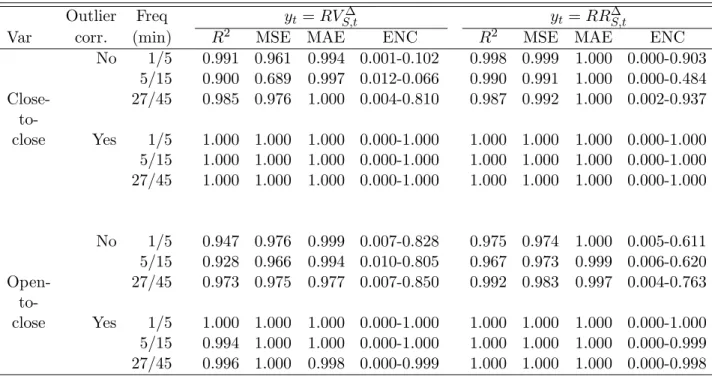
To compare the realized range and realized variance estimators with the proce-dure outlined above several variants are tested. First, three sampling frequencies are considered: 1/5 (one-minute intervals from 9:30-16:15 EST, five-minute intervals from 16:15-9:30 EST), 5/15, and 27/45 minutes. Second, the issue of market closure is addressed by not only looking at the close-to-close 24-hour day, but also only at the open-to-close period (9:30-16:15 EST for the S&P500 index-futures, 9:30-16:00 EST for the individual stocks in Section 5). Third, closely related to this is the presence of large outliers in especially the realized variance series of the individual stocks for the close-to-close period, often caused by a large overnight return. Therefore next
to the unadjusted series results are also reported when all variance measures are truncated at the median plus or minus four times the median absolute deviation.2
The results for the S&P500 index-futures are reported in Tables 8 to 13. Re-gardless of the sampling frequency, the outlier adjustments, or close-to-close versus open-to-close, the unadjusted realized range performs significantly better than the realized variance with only a few exceptions, as shown in Table 8. The main ex-ceptions are at the one-minute frequency with realized variance as the forecasting target yt and the MSE or MAE as performance measures. This can be explained
by the fact that the realized range is severely downward biased at the one-minute frequency as shown in Table 7. The logical next step is therefore to look at the scaled versions of the realized variance and the realized range in Table 9. Here we do see an improved performance of the realized range at the one-minute frequency. The overall picture remains that the (scaled) realized range is superior. The encompass-ing regressions even suggest the (scaled) realized variance contains no incremental information beyond that already captured by the (scaled) realized range.
insert Tables 810 about here
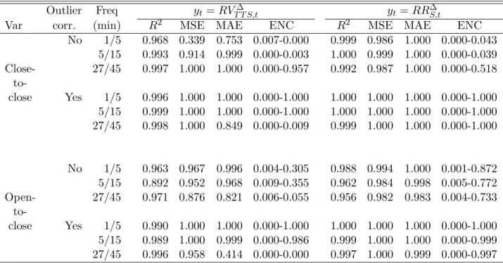
-In the simulation experiments in Section 3 we found that the TTS estimator came closest to the performance of the scaled realized range in the presence of market microstructure noise. Table 10 reports the corresponding results for the S&P500, showing that also for this empirical application the TTS estimator does a better job than the (scaled) realized variance. Still the number of significant results in Table 10 is 61-4 in favour of the scaled realized range. This is perhaps a bit surprising in light of the simulation results. In our opinion, it mainly illustrates the robustness of scaling as a bias-adjustment procedure compared to a bias-corrected estimator based on specific model assumptions. The data generating process in our simulation experiment exactly satisfies the conditions under which the TTS estimator was derived, but the actual data probably do not completely adhere to
2See Hansen and Lunde (2006a) and Patton (2005) for extensive discussion of pitfalls in forecast
those conditions.
So far we considered random walk forecasts. Tables 11 to 13 provide the cor-responding results for the rolling forecasts following the procedure of Fleming et al. (2003). Here the improved forecast performance of the (scaled) realized range relative to the (scaled) realized variance and the TTS estimator are even more pro-nounced than before. Counting the number of significant results across the entire table we now get 74-5 in Table 11 (was 77-6 in Table 8), 92-0 in Table 12 (was 80-1 in Table 9), and 82-0 in Table 13 (was 61-4 in Table 10), all in favour of the realized range.
insert Tables 1113 about here
-5
S&P100 constituents
Obviously the analysis in the previous section only considers 1 particular asset, the S&P500 index-futures, which is an extremely liquid asset with a small bid-ask spread. With the main issue at stake being whether the realized range better deals with market microstructure than the realized variance this could provide a biased picture. For that reason we also consider the individual stocks in the S&P100 index (constituents in June 2004), where the data consists of open, high, low and close transaction prices at the one-minute frequency. For most stocks the sample period runs from April 9, 1997, to June 18, 2004 (1808 daily observations). Table 14 reports some sample statistics on the distribution of the 100 (scaled) realized ranges based on the five-minute frequency from 9:30 to 16:00 EST, in addition to the close-to-open squared return. This table is similar in nature to the one in ABDE for the realized variance of the 30 Dow Jones stocks.
insert Table 14 about here
-The average realized range at 4.798 and the average standard deviation of the range at 3.637 are both larger for the individual stocks compared to that for the S&P500 index-futures. The large skewness and kurtosis is partly the result of large
overnight returns after disappointing firm-specific news announcements. The general features are similar for the scaled realized range. Obviously for stocks where the infrequent trading bias dominates the mean is scaled upwards (e.g. in the lowest percentile), and for stocks where the bid-ask bounce bias dominates the mean is scaled downwards (e.g. in the highest percentile).
Again we compare the realized range and realized variance, along the lines de-scribed in Section 4. We do not consider the two time-scale estimator here as the highest available sampling frequency only is one minute. The results are presented in Table 15 to 17, where we record a DM test either as a win for realized variance (1-0), a win for realized range (0-1), or undecided (0-0) using a 5% significance level in a one-sided test. Note that for the encompassing test it is possible that both score a win (1-1). The results in Table 15 indicate that in particular for the popular five-and 30-minute frequencies the realized range performs significantly better than the realized variance. Only for the one-minute frequency the realized variance performs significantly better than the realized range when realized variance is used to evalu-ate both, whereas the realized range outperforms the realized variance when realized range is used to evaluate both. Of all significant differences 80% are in favour of the realized range.
insert Tables 1516 about here
-Table 16 shows the results for the scaled versions of the realized variance and the realized range. The results are similar to the ones in 15 in the sense that still about 80% of the significant differences are in favour of the scaled realized range. There are, however, a few notable differences. Most of these occur when using the MSE and MAE, where the volatility measure that is not used as the forecast target is now more often winning. A logical explanation for this is that these measures increase for large differences in the levels of the actual volatility and the forecast. As we already have seen in the simulation experiments at the highest frequencies we consider here the realized range has a higher average than the realized variance in the presence of both non-trading and bid-ask bounce. This difference is removed
when using the scaled versions.
Producing rolling forecasts following Fleming et al. (2003), Table 17 clearly favours the realized range. Now 88% of all significant results favour the realized range. The additional gains come especially for the R-squared and the encompass-ing regression measures.
insert Table 17 about here
-To further analyse the effect of non-trading on the realized range, we look at the relation between trading activity in a stock and the win-loss ratio. In particular we construct a variable that counts per stock the number of wins for the realized variance minus the number of wins for the realized range, taken over all instances covered by Tables 15 to 17 (so open-to-close, with and without outliers, etc.). We measure trading activity by the average number of minutes per day without a trade. When regressing the win-loss difference on this (non-)trading activity variable we find a statistically significant negative relationship. Hence, the realized range is more likely to win if a stock is more actively traded. Obviously in this case we move closer to the S&P500 example where results were strongly in favour for the realized range.
6
Concluding remarks
In this paper we studied the properties and merits of the ‘realized range’, a measure of daily volatility computed by summing high-low ranges for intra-day intervals. In theory the high-low range is a more efficient estimator of volatility than the squared return. Hence, just like the daily high-low range improves over the daily squared return, the ‘realized range’ should improve over the ‘realized variance’ obtained by summing squared returns for intra-day intervals. Theoretically that is. In practice we need to account for market frictions such as bid-ask bounce and infrequent trading. For this purpose, we proposed a bias-adjustment procedure for the realized range estimator, which involves scaling the realized range with the ratio of the average level of the daily range and the average level of the realized range.
A simulation experiment first confirms that in theory indeed the realized range is a better volatility measure than the realized variance when using the same sampling frequency. This no longer is true for the highest sampling frequencies in the case of infrequent trading as this leads to a downward bias in the realized range and does not affect the realized variance. When allowing for bid-ask bounce both realized range and realized variance are upward biased, but the realized range suffers more as the minimum (maximum) is often half a spread below (above) the true minimum (maximum). In the presence of these market microstructure frictions, scaling the realized range with the average (relative) level of the daily range turns out to be an effective procedure to remove the induced bias and restore the efficiency of the real-ized range. In particular, the scaled realreal-ized range outperforms popular corrections of the realized variance for microstructure noise, including the two time-scales esti-mator of Zhang et al. (2005) and the kernel-based estiesti-mators considered by Hansen and Lunde (2006b).
For the S&P500 index-futures we come closest in practice to the ideal situation of continuous trading and no market frictions. As expected the simulation results are confirmed in that the (scaled) realized range improves significantly over the (scaled) realized variance as well as the two time-scales estimator as a measure for daily volatility. For the constituents of the S&P100 index all ingredients of market frictions are present, with bid-ask bounce, discontinuous trading and large (overnight) jumps. The results are more mixed here, but realized range still significantly improves over realized variance for the popular sampling frequencies of five and 30 minutes.
References
A¨ıt-Sahalia, Y., P.A. Mykland and L. Zhang, 2005, How often to sample a continuous-time process in the presence of market microstructure noise. Review of Financial Studies 18, 351–416.
Alizadeh, S., 1998, Essays in Financial Econometrics. Department of Economics, Univer-sity of Pennsylvania, Ph.D. Dissertation.
Alizadeh, S., M.W. Brandt and F.X. Diebold, 2002, Range-based estimation of stochastic volatility models. Journal of Finance 47, 1047–1092.
Andersen, T.G. and T. Bollerslev, 1998, Answering the skeptics: Yes, standard volatility models do provide accurate forecasts. International Economic Review 39, 885–905. Andersen, T.G., T. Bollerslev, F.X. Diebold and H. Ebens, 2001a, The distribution of
realized stock return volatility. Journal of Financial Economics 61, 43–76.
Andersen, T.G., T. Bollerslev, F.X. Diebold and P. Labys, 2001b. The distribution of realized exchange rate volatility. Journal of the American Statistical Association 96, 42–55.
Andersen, T.G., T. Bollerslev, F.X. Diebold and P. Labys, 2003, Modeling and forecasting realized volatility. Econometrica 71, 579–625.
Andreou, E. and E. Ghysels, 2002, Rolling-sample volatility estimators: some new theo-retical, simulation and empirical results. Journal of Business and Economic Statistics 20, 363–376.
Bali, T.G. and D. Weinbaum, 2005, A comparative study of alternative extreme-value volatility estimators. Journal of Futures Markets 25, 873–892.
Bandi, F.M. and J.R. Russell, 2005a, Microstructure noise, realized variance, and optimal sampling. Graduate School of Business, University of Chicago, working paper.
Bandi, F.M. and J.R. Russell, 2005b, Separating microstructure noise from volatility. Jour-nal of Financial Economics, to appear.
Barndorff-Nielsen, O.E. and N. Shephard, 2002, Econometric analysis of realised volatility and its use in estimating stochastic volatility models. Journal of the Royal Statistical Society Series B 64, 253–280.
Barndorff-Nielsen, O.E., P.R. Hansen, A. Lunde and N. Shephard, 2004, Regular and modified kernel-based estimators of integrated variance: The case of independent noise. Oxford Financial Research Centre Economics Series 2004-FE-20.
Beckers, S., 1983, Variances of security price returns based on high, low, and closing prices. Journal of Business 56, 97–112.
Brandt, M.W. and F.X. Diebold, 2006, A no-arbitrage approach to range-based estimation of return covariances and correlations. Journal of Business 79, 61–74.
Brown, S., 1990, Estimating volatility, in: S. Figlewski, W. Silber and M. Subramanyam, (Eds.), Financial options: From theory to practice, Business One Irwin, Homewood IL., pp. 516–537.
Christensen, K. and M. Podolskij, 2005, Realized range-based estimation of integrated variance. Aarhus School of Business, manuscript.
Diebold, F.X. and R.S. Mariano, 1995, Comparing predictive accuracy. Journal of Business and Economic Statistics 13, 253–263.
Fleming, J., C. Kirby and B. Ostdiek, 2003, The economic value of volatility timing using ‘realized’ volatility. Journal of Financial Economics 67, 473–509.
Foster, D.P. and D.B. Nelson, 1996, Continuous record asymptotics for rolling sample variance estimators. Econometrica 64, 139–174.
Garman, M.B. and M.J. Klass, 1980, On the estimation of security price volatilities from historical data. Journal of Business 53, 67–78.
Hansen, P.R. and A. Lunde, 2005, A realized variance for the whole day based on inter-mittent high-frequency data. Journal of Financial Econometrics 3, 525–554.
Hansen, P.R. and A. Lunde, 2006a, Consistent ranking of volatility models. Journal of Econometrics, to appear.
Hansen, P.R. and A. Lunde, 2006b, Realized variance and market microstructure noise. Journal of Business and Economic Statistics, to appear.
Harvey, D.I., S.J. Leybourne and P. Newbold, 1998, Tests for forecast encompassing. Journal of Business and Economic Statistics 16, 254–259.
Kunitomo, N., 1992, Improving the Parkinson method of estimating security price volatilites. Journal of Business 65, 295–302.
Parkinson, M., 1980, The extreme value method for estimating the variance of the rate of return. Journal of Business 53, 61–65.
Patton, A., 2005, Volatility forecast evaluation and comparison using imperfect volatility proxies. London School of Economics, manuscript.
Rogers, L.C.G. and S.E. Satchell, 1991, Estimating variance from high, low and closing prices. Annals of Applied Probability 1, 504–512.
Yang, Z. and Q. Zhang, 2000, Drift-independent volatility estimation based on high, low, open, and close prices. Journal of Business 73, 477–491.
Zhang, L., P.A. Mykland and Y. A¨ıt-Sahalia, 2005, A tale of two time scales: Determining integrated volatility with noisy high-frequency data. Journal of the American Statistical Association 100, 1394–1411.
Table 1: Realized range and realized variance with continuous trading and no market frictions
Frequency RR∆t RR∆S,t RVt∆ RVS,t∆ RVT T S,t∆ RVAC∆1,t
(minutes) Mean RMSE Mean RMSE Mean RMSE Mean RMSE Mean RMSE Mean RMSE 1 4.333 0.105 4.299 0.135 4.411 0.155 4.317 0.197 4.413 0.145 4.429 0.258 2 4.356 0.112 4.299 0.150 4.418 0.213 4.318 0.242 4.421 0.185 4.448 0.389 3 4.368 0.128 4.299 0.165 4.428 0.269 4.319 0.289 4.428 0.224 4.448 0.468 4 4.379 0.143 4.300 0.179 4.441 0.325 4.320 0.337 4.435 0.259 4.444 0.547 5 4.382 0.156 4.299 0.189 4.431 0.347 4.317 0.358 4.439 0.287 4.434 0.615 10 4.402 0.217 4.300 0.240 4.432 0.501 4.320 0.502 4.436 0.406 4.378 0.915 15 4.405 0.271 4.300 0.288 4.419 0.638 4.317 0.636 4.425 0.510 4.456 1.130 20 4.409 0.314 4.302 0.326 4.411 0.740 4.325 0.734 4.410 0.603 4.514 1.304 30 4.409 0.393 4.298 0.400 4.435 0.908 4.315 0.893 4.441 0.749 4.455 1.585 45 4.425 0.490 4.301 0.489 4.493 1.148 4.322 1.109 4.475 0.933 4.332 1.929 60 4.425 0.579 4.299 0.574 4.444 1.315 4.316 1.283 4.445 1.079 4.292 2.190 90 4.435 0.714 4.300 0.701 4.420 1.625 4.320 1.591 4.401 1.338 4.214 2.538 120 4.418 0.827 4.297 0.813 4.372 1.809 4.317 1.789 4.360 1.528 4.146 2.792 180 4.399 1.005 4.300 0.989 4.313 2.192 4.319 2.195 4.305 1.800 4.149 3.454 240 4.362 1.128 4.296 1.116 4.230 2.423 4.311 2.465 4.251 2.048 4.242 3.913 360 4.341 1.317 4.294 1.306 4.192 2.878 4.311 2.954 4.233 2.627 4.307 4.687 720 4.331 1.889 4.298 1.877 4.318 4.330 4.330 4.347 4.231 4.190 4.323 5.664 1440 4.287 2.564 4.287 2.564 4.323 5.664 4.323 5.664 4.323 5.664 4.323 5.664 Note: The table shows the results of a simulation experiment where 5000 days of 8,640,000 (log) prices (100 prices per second) are simulated from a normal distribution with mean zero and variance 4.41 (21% standard deviation on an annual basis). All prices are observed. For each day the realized range (RR∆
t ), the scaled realized range (RRS,t∆), the realized variance (RVt∆), the scaled realized variance (RVS,t∆), the two time-scales estimator (RVT T S,t∆ ) and the first-order kernel-based estimator (RVAC∆1,t) are computed for various sampling frequencies shown in column 1. RR∆S,tandRVS,t∆ are obtained from (11) withq= 5000 (withRRreplaced byRV
for the scaled realized variance).
Table 2: Realized range and realized variance with infrequent trading
Frequency RR∆t RR∆S,t RVt∆ RVS,t∆ RVT T S,t∆ RVAC∆1,t
(minutes) Mean RMSE Mean RMSE Mean RMSE Mean RMSE Mean RMSE Mean RMSE 1 2.633 1.778 4.317 0.137 4.412 0.162 4.262 0.217 4.411 0.154 4.409 0.282 2 3.034 1.379 4.317 0.157 4.409 0.229 4.263 0.267 4.411 0.202 4.407 0.396 3 3.241 1.174 4.316 0.177 4.413 0.281 4.261 0.310 4.410 0.240 4.403 0.481 4 3.372 1.046 4.316 0.192 4.406 0.323 4.258 0.348 4.409 0.274 4.409 0.554 5 3.468 0.953 4.318 0.205 4.407 0.361 4.263 0.380 4.408 0.303 4.414 0.623 10 3.712 0.730 4.314 0.266 4.402 0.509 4.253 0.517 4.411 0.419 4.431 0.889 15 3.835 0.633 4.318 0.313 4.421 0.626 4.265 0.622 4.417 0.517 4.452 1.086 20 3.903 0.594 4.314 0.356 4.412 0.721 4.253 0.713 4.422 0.598 4.451 1.281 30 3.995 0.566 4.318 0.426 4.438 0.893 4.271 0.871 4.429 0.734 4.455 1.589 45 4.074 0.582 4.319 0.512 4.437 1.094 4.264 1.062 4.439 0.915 4.443 1.942 60 4.121 0.628 4.320 0.592 4.439 1.283 4.265 1.241 4.442 1.069 4.433 2.216 90 4.175 0.724 4.316 0.715 4.432 1.585 4.260 1.531 4.445 1.332 4.390 2.745 120 4.216 0.815 4.322 0.817 4.423 1.815 4.272 1.759 4.434 1.561 4.421 3.127 180 4.246 1.010 4.327 1.020 4.403 2.270 4.276 2.209 4.417 1.955 4.501 3.782 240 4.275 1.151 4.329 1.161 4.417 2.598 4.297 2.530 4.413 2.309 4.514 4.233 360 4.298 1.429 4.335 1.439 4.445 3.213 4.294 3.106 4.474 2.942 4.450 5.078 720 4.354 2.024 4.342 2.019 4.430 4.503 4.319 4.392 4.453 4.524 4.342 6.186 1440 4.353 2.799 4.353 2.799 4.342 6.186 4.342 6.186 4.342 6.186 4.342 6.186 Note: The table shows the results of a simulation experiment where 5000 days of 8,640,000 (log) prices (100 prices per second) are simulated from a normal distribution with mean zero and variance 4.41 (21% standard deviation on an annual basis). Subsequently, with probability π = 0.001 we observe a price and with probability 1−π we do not. For each day the realized range (RR∆
t ), the scaled realized range (RR∆S,t), the realized variance (RVt∆), the scaled realized variance (RVS,t∆), the two time-scales estimator (RV∆
T T S,t) and the first-order kernel-based estimator (RVAC∆1,t) are computed for various sampling frequencies shown in column 1.
RR∆
S,tandRVS,t∆ are obtained from (11) with q= 5000 (withRRreplaced byRV for the scaled realized variance).
Table 3: Realized range and realized variance with bid-ask bounce
Frequency RR∆t RR∆S,t RVt∆ RVS,t∆ RVT T S,t∆ RVAC∆1,t
(minutes) Mean RMSE Mean RMSE Mean RMSE Mean RMSE Mean RMSE Mean RMSE 1 14.682 10.273 4.490 0.099 8.913 4.514 4.319 0.196 4.419 0.217 4.429 0.389 2 11.024 6.616 4.490 0.109 6.664 2.277 4.320 0.247 4.426 0.215 4.450 0.467 3 9.579 5.172 4.490 0.121 5.931 1.564 4.321 0.294 4.432 0.241 4.445 0.532 4 8.772 4.366 4.490 0.132 5.565 1.224 4.320 0.337 4.438 0.270 4.444 0.605 5 8.237 3.832 4.490 0.142 5.331 1.013 4.320 0.362 4.442 0.295 4.437 0.663 10 6.999 2.603 4.491 0.193 4.883 0.725 4.322 0.501 4.440 0.409 4.382 0.945 15 6.479 2.094 4.491 0.240 4.721 0.746 4.321 0.633 4.428 0.512 4.460 1.149 20 6.182 1.809 4.492 0.280 4.632 0.810 4.327 0.735 4.414 0.604 4.514 1.328 30 5.832 1.490 4.489 0.354 4.586 0.950 4.319 0.889 4.444 0.750 4.460 1.606 45 5.572 1.283 4.492 0.447 4.591 1.178 4.322 1.104 4.478 0.934 4.337 1.945 60 5.410 1.184 4.490 0.533 4.518 1.336 4.319 1.279 4.449 1.080 4.293 2.201 90 5.232 1.126 4.490 0.666 4.471 1.644 4.323 1.591 4.404 1.339 4.213 2.548 120 5.104 1.123 4.488 0.782 4.410 1.826 4.317 1.791 4.363 1.528 4.149 2.805 180 4.954 1.192 4.490 0.966 4.338 2.201 4.321 2.194 4.308 1.800 4.148 3.468 240 4.839 1.257 4.487 1.099 4.246 2.425 4.311 2.460 4.254 2.048 4.249 3.932 360 4.727 1.405 4.485 1.300 4.201 2.885 4.314 2.957 4.236 2.627 4.316 4.696 720 4.602 1.948 4.489 1.894 4.325 4.343 4.331 4.353 4.234 4.191 4.327 5.679 1440 4.478 2.613 4.478 2.613 4.327 5.679 4.327 5.679 4.327 5.679 4.327 5.679 Note: The table shows the results of a simulation experiment where 5000 days of 8,640,000 (log) prices (100 prices per second) are simulated from a normal distribution with mean zero and variance 4.41 (21% standard deviation on an annual basis). All prices are observed, but are converted to bid and ask prices (with equal probability) by either subtracting or adding half the spreads= 0.005 (on a starting price of 1). For each day the realized range (RR∆
t ), the scaled realized range (RR∆S,t), the realized variance (RVt∆), the scaled realized variance (RVS,t∆), the two time-scales estimator (RVT T S,t∆ ) and the first-order kernel-based estimator (RVAC∆1,t) are computed for various sampling frequencies shown in column 1. RR∆S,tandRVS,t∆ are obtained from (11) with q= 5000 (withRR
replaced byRV for the scaled realized variance).
Table 4: Realized range and realized variance with infrequent trading and bid-ask bounce
Frequency RR∆t RR∆S,t RVt∆ RVS,t∆ RVT T S,t∆ RVAC∆1,t
(minutes) Mean RMSE Mean RMSE Mean RMSE Mean RMSE Mean RMSE Mean RMSE 1 8.243 3.836 4.472 0.097 8.913 4.515 4.263 0.213 4.415 0.205 4.419 0.401 2 7.073 2.667 4.473 0.110 6.664 2.280 4.264 0.265 4.416 0.219 4.402 0.475 3 6.562 2.158 4.472 0.127 5.917 1.553 4.263 0.310 4.414 0.250 4.410 0.541 4 6.258 1.856 4.472 0.140 5.529 1.190 4.258 0.349 4.412 0.279 4.414 0.605 5 6.056 1.657 4.473 0.156 5.311 1.001 4.264 0.381 4.411 0.306 4.417 0.667 10 5.553 1.172 4.471 0.216 4.853 0.717 4.255 0.519 4.414 0.420 4.436 0.923 15 5.344 0.984 4.474 0.267 4.723 0.742 4.266 0.626 4.420 0.518 4.463 1.112 20 5.212 0.877 4.471 0.310 4.636 0.793 4.255 0.715 4.425 0.598 4.454 1.302 30 5.066 0.784 4.474 0.385 4.597 0.944 4.274 0.872 4.432 0.735 4.457 1.606 45 4.950 0.749 4.474 0.474 4.537 1.129 4.262 1.064 4.442 0.915 4.445 1.957 60 4.881 0.765 4.476 0.556 4.518 1.306 4.266 1.238 4.445 1.069 4.435 2.225 90 4.794 0.824 4.471 0.683 4.486 1.607 4.259 1.532 4.448 1.332 4.393 2.760 120 4.755 0.904 4.478 0.790 4.464 1.828 4.274 1.756 4.437 1.561 4.417 3.138 180 4.686 1.077 4.481 0.999 4.429 2.279 4.276 2.205 4.420 1.955 4.506 3.787 240 4.657 1.214 4.484 1.147 4.434 2.604 4.296 2.526 4.416 2.309 4.518 4.240 360 4.609 1.483 4.490 1.434 4.460 3.223 4.296 3.107 4.477 2.942 4.453 5.087 720 4.574 2.075 4.498 2.035 4.436 4.510 4.318 4.391 4.456 4.524 4.340 6.189 1440 4.509 2.844 4.509 2.844 4.340 6.189 4.340 6.189 4.340 6.189 4.340 6.189 Note: The table shows the results of a simulation experiment where 5000 days of 8,640,000 (log) prices (100 prices per second) are simulated from a normal distribution with mean zero and variance 4.41 (21% standard deviation on an annual basis). Subsequently with probabilityπ= 0.001 we observe a price and with probability 1−πwe do not, while the observed prices converted to bid and ask prices (with equal probability) by either subtracting or adding half the spread s= 0.005 (on a starting price of 1). For each day the realized range (RR∆
t ), the scaled realized range (RR∆S,t), the realized variance (RVt∆), the scaled realized variance (RVS,t∆), the two time-scales estimator (RVT T S,t∆ ) and the first-order kernel-based estimator (RVAC∆1,t) are computed for various sampling frequencies shown in column 1. RR∆S,t and RVS,t∆ are obtained from (11) with q= 5000 (with RRreplaced by RV for the scaled realized variance).