Portfolio Optimisation Using Value at Risk

Portfolio Optimisation Using

Value at Risk

Project Report

by

Vinay Kaura

A project report submitted as partial fulfilment of the requirements for the degree of Computing (Computational Management) MEng

Imperial College London Project Supervisor: Prof. Berç Rustem

Second Marker: Panayiotis Parpas

Abstract

Optimal portfolios are normally computed using the portfolio risk measured in terms of its variance. However, performance risk is a problem if the portfolio does not perform well. This project involves using linear programming techniques to define and handle the “Value-At-Risk” risk metric.

By evaluating historical prices to create future scenarios one can determine the “Value-At-Risk” of a specified portfolio. Using linear programming software to develop a returns model for the FTSE 100 one can, hence, calculate which stocks should be bought or sold in order to minimise the “Value-At-Risk” of a portfolio with an underlying required returns constraint. The developed tool will look at multi-period scenarios and seek to optimise the portfolio accordingly.

This report documents the analysis of current ways of measuring single period “Value-At-Risk” and the formulation of a unique method of calculating multi-period “Value-At-“Value-At-Risk”. It goes on to describe an application which implements this model and highlights the results of exhaustive testing of the application.

Ultimately, using back testing, this report demonstrates how the developed model would have, hypothetically, been able to make profits of up to 40% over the course of the past year while the FTSE 100 benchmark rose by only 27%.

Acknowledgements

Throughout the duration of this project Professor Berç Rustem has been a brilliant project supervisor and his vast array of knowledge has been a great help in times of need. I am also very grateful for the advice given by Panayiotis Parpas during my project.

For the assistance given in setting up of batch jobs and discussing technical implementation techniques I would like to thank Duncan White from CSG.

I would also like to thank Rezwan Ud-Din, from Goldman Sachs, who took time out of his busy schedule to test my final application.

Table of Contents

1. Introduction

1.1. Introduction & Motivation ...1

1.2. Project Objectives ...3

1.3. Key Contributions ...3

2. Background Research 2.1. Value At Risk and Current Implementations ...4

2.2. Conditional Value At Risk ...8

2.3. Multi-period Scenario Generation & Portfolio Representation...11

2.4. Multi-period Optimisation ...13

2.5. Efficient Frontier ...14

3. Specification 3.1. Core Requirements 3.1.1.Core Requirements – Front-End Specification ...16

3.1.2.Core Requirements – Back-End Specification ...17

3.2. Non-Core Requirements ...17 3.3. Extensions ...18 3.4. Documentation Requirements ...18 3.5. Implementation Requirements ...19 3.6. Summary of Requirements ...19 4. System Design 4.1. System Overview ...20 4.2. Component Organisation ...22

4.3. Graphical User Interface ...23

5. System Implementation 5.1. Implementation Languages ...25 5.2. The Database 5.2.1.Database Implementation ...25 5.2.2.Database Structure ...27 5.2.3.Database API ...28

5.3. The Data Downloader 5.3.1.Data Source ...29

5.3.2.Data Acquisition ...29

5.3.3.Parameters Re-calculation ...30

5.3.4.Job Automation ...30

5.4. The Scenario Generator 5.4.1.Cluster ...30

5.4.2.Java Wrapper ...31

5.5. The Optimiser 5.5.1.Optimisation Library Selection ...33

5.5.2.Interlinking the Optimisation Library with the Application ...34

5.5.3.Optimiser Wrapper ...35

5.6. The Graphical User Interface 5.6.1.Interface Concepts ...37

5.6.2.Application Graphical User Interface ...37

5.6.3.Current Portfolio Composition & Parameters Panel ...39

5.6.4.Scenario Tree Panel ...41

5.6.5.Optimised Portfolio Panel ...42

5.6.6.Portfolio History Panel ...45

5.6.7.Historical Asset Prices Panel ...45

5.6.8.Back Testing Panel ...46

5.6.9.JFreeChart Graphs ...47

5.7. The Back Tester ...48

6. Project Management 6.1. Source Control ...49

6.2. Time Management ...49

7. Testing & Evaluation 7.1. Model Verification 7.1.1.Individual Optimisations ...51

7.1.2.Back Testing ...52

7.1.3.Efficient Frontier ...55

7.2. Validation of the Interface and System Features ...56

7.3. End User Testing: Demonstration to Goldman Sachs ...58

7.4. Summary ...59 8. Conclusion 8.1. Remarks ...60 8.2. Future Work ...60 9. References ...61 10. Appendix 10.1. Section A: Stored Procedures ...62

10.2. Section B: Example Auto-Generated Optimisation Output File...63

10.3. Section C: Feedback Email From Rezwan Ud-Din ...64

Chapter 1

Introduction

1.1 Introduction & Motivation

Before looking at “Value at Risk” (VaR), we need to firstly define what risk is and, secondly, why we require a method to measure it. With regards to this project, risk is a measure of how volatile an asset’s returns are. Exposure to this volatility can lead to a loss in ones investments. For this reason tools are used not only to passively measure and report risk, but also to defensively control or actively manage it.

As stated in [6] and [7], there have been several large publicised losses in the 1990s, all of which have highlighted the need for accurate risk measure and control. These have included:

ƒ In February 1993, Japan’s Showa Shell Sekiyu oil company losing $1.58Billion from speculating on exchange rates.

ƒ In December 1993, MG Refining and Marketing reporting a loss of $1.3Billion from failed hedging of long-dated oil supply commitments.

ƒ In December 1994, California’s Orange County announcing losses from repos and other transactions totalling $1.8Billion.

ƒ In February 1995, Nick Leeson, a trader from Britain’s Barings PLC, losing $1.33Billion from unauthorised Nikkei futures trading.

After such events regulators have sought to defensively control the risk institutions take. They aim to find a balance between setting out a comprehensive set of regulations to identify institutions who take on excessive risk, while not introducing too rigid a system.

VaR is a popular method which regulators use to assess risk. For example, the Basle Committee1 _{has sanctioned institutions to use internal VaR models for capital requirements}2_.

VaR is also used by institutions themselves. It is commonly used for self-regulation in the following manner:

ƒ Benchmark Measure – To provide a company-wide yardstick to compare risks across different markets.

ƒ Potential Loss Measure – To give a broad idea of the worst loss an institution can incur.

ƒ Equity Capital – To set a capital cushion for the institution.

When managed properly, VaR can provide a controlled way of getting high returns on ones investments. In March 2006, David Viniar, Chief Financial Officer from the investment bank Goldman Sachs, stated that the firm’s VaR rose from $80million in the previous quarter to $92million (+15%), which allowed the firm to increase its net income by 64%.

1 _{Committee set up by the Bank of International Settlements and based in Basle. It drew up international capital adequacy}

standards for banks. As stated on http://www.finance-glossary.com.

2 _{Rules to identify how much risk the bank is exposed to and then make sure if it loses money then it has enough in reserves}

However, rather than just using VaR to measure the risk of institutions as a whole, it is also used by institutions in portfolio optimisation techniques to actively manage their risk. This is the focus of my project.

Modern Portfolio Theory models the return of an asset as a random variable and a portfolio as a weighted combination of these assets1_{. This implies that the return of a portfolio is thus}

also a random variable and consequently has an expected value and a variance. Risk in this model is normally identified with the variance of portfolio return. However, for the purposes of my project, VaR will be used to define the risk of portfolios.

The main problem with variance is that it does not take into consideration the direction of an investment's movement. An asset could be volatile because its price rises quickly, however investors are not distressed by gains!

For investors, risk is about the odds of losing money, and VaR is based on that common-sense fact. By assuming that investors care about the odds of big losses, VaR can be used to answer the questions, "What is my worst-case scenario?" or "How much could I lose in a really bad month?"

The VaR statistic has three components: a time period, a confidence level and a loss amount (or loss percentage). It can thus be used to answer question such as:

ƒ What is the most I can (with a 95% or 99% level of confidence) expect to lose in pounds over the next month?

ƒ What is the maximum percentage I can (with 95% or 99% confidence) expect to lose over the next year?

Bearing this risk measure in mind, I aim to develop an application that will recommend rational investment decisions. Rationality is modelled by supposing that an investor choosing between several portfolios with identical expected returns, will prefer that portfolio which minimizes risk.

By discretising the future into scenarios comprising of multiple time periods, investment decisions will need to be made at the beginning of each period. Using Linear Programming techniques, an objective function and set of constraints will be generated to represent the investment problem. Making use of optimisation software, the optimal parameters for the decisions will then be determined.

This is a risky project since there does not exist at present a similar multi-period portfolio optimisation model which takes into consideration VaR. Combining the representation of a multi-period portfolio with the calculation of VaR, this report defines a model which can optimise a portfolio to hopefully provide lucrative returns.

It's not whether you're right or wrong that's important, but how much money you make when you're right and how much you lose when you're wrong. - George Soros

1.2 Project Objectives

The project has the following key objectives:

ƒ Analyse the current methods of calculating single period VaR and formulate a new multi-period optimisation model

ƒ Implement the developed model as an easy to use application

ƒ Implement an automated back-testing facility to verify the accuracy of the developed model

ƒ Demonstrate how the application could be incorporated into a professional Portfolio Manager’s daily workflow

1.3 Key Contributions

This report is divided up into the following key chapters:

Background Research

The background research introduces various methods in which VaR is currently calculated and how it can be applied to portfolio optimisations. It also explains that VaR has adverse properties which makes it difficult to use in portfolio optimisations. “Conditional Value-At-Risk” (CVaR) is introduced as an alternative method of calculating VaR. We then go onto discuss the multi-period portfolio optimisation problem and finally combine the multi-period portfolio representation with the calculation of CVaR to define a new multi-period portfolio optimisation model using CVaR.

System Design

The formulated model will only be useful to a user if it is incorporated in a well designed application. This chapter describes a proposed application which seeks to demonstrate how a professional portfolio manager could use the model to make investment decisions and contains features which would allow the use of the application to fit in the portfolio manager’s normal day-to-day work patterns.

System Implementation

This chapter describes how the various modules of the application were implemented, and highlights the problems encountered and how they were rectified.

Testing & Evaluation

The project’s testing is split into testing of the model, through back-testing, and testing of the application, through exhaustive and user testing. This chapter describes the tests carried out, and their results and analysis.

Conclusion

This chapter analyses the overall project and comments upon its strengths and weaknesses. It also highlights suggestions for future work which could be carried out to further enhance the developed application and model.

Chapter 2

Background Research

Investing without research is like playing stud poker and never looking at the cards. Peter Lynch

2.1 Value at Risk and Current Implementations

Formally put, “Value-at-Risk” (VaR) measures the worst expected loss over a given horizon under normal market conditions at a given confidence level, as stated in [12].

To put this into context, one might say that the VaR of their portfolio is £0.5 million at the 95% confidence level with the target horizon set to one week. This means that there is a 5 out of 100 chance that the portfolio will lose over £0.5 million within the target horizon under normal market conditions.

Figure 1, below, visually highlights this. It displays 520 observations of the return of a portfolio with the target horizon set to one week. The VaR of the portfolio is the loss that will not be exceeded in 95% of the cases, ie. the lower 5% of returns (26 largest losses), which is equal to £0.5 million.

Figure 1

One method of estimating the VaR is to assume that the distribution of returns of the portfolio follows a Normal Distribution. Hence, we can multiply the standard deviation of the returns (3.19) by the 95 percentile of the standard normal distribution (1.645) and subtract this from the mean of the returns (5.55). In this example, this method would estimate the VaR of the portfolio to be £0.3 million.

VaR is a popular risk measure as it provides users with a summary measure of market risk using the same units as the portfolio’s bottom line; eg. GBP, USD or EUR depending upon the base currency of the portfolio. This means that VaR can also be communicated to a relatively non-technical audience, such as managers or shareholders.

VaR is also favourable as it looks at downside risk. Hence, unlike the variance of a portfolio, it is not impacted by high returns.

0 20 40 60 80 100 120 -5 -4 -3 -2 -1 0 1 2 3 4 5 6 7 8 9 10 11 12 13 14

Weekly Return (£million)

Numb er o f O ccu re nc es 5% loss probability

-2 2 4 6 8 0.05 0.1 0.15 0.2 ξ µ 2σ p(ξ) VaR area = 1-α

In order to analyse VaR further, we can mathematically define it as:

VaR=ζ_α(ξ)=inf{ζ |P(ξ≤ζ)≥α} (1)

where αis the confidence level and ξ is a random variable

As mentioned earlier, we could assume the rate of returns of a portfolio could follow a normal distribution, in which case the VaR of the portfolio would be1_:

ζ_α(ξ) 1(α) µ (α)σ k VaR= =Φ− = + (2) s.t. (_α)₌ 2 −1(2_α−1) erf k (3) =

∫

− z t dt e z erf 0 2 2 ) ( π (4)

where ξ is a randomly distributed variable with mean µand standard deviation σ

The problem with this assumption is that the normal distribution curve assumes each event is completely random. However, in reality, when a share price falls, people sell. This extra surge of selling will push the share price into the extremes a lot quicker than the curve suggests. A similar thing will happen when a share price rises. To overcome this problem, rather than using a parametric approach, implementations can use an empirical approach to calculate a portfolio’s current risk.

As stated in [3], three common ways of calculating VaR are: ƒ Variance covariance

ƒ Historical

ƒ Stochastic or Monte Carlo simulation

The variance covariance method uses information on the volatility and correlation of stocks to compute the VaR of a portfolio. The volatility of an asset is a measure of the degree to which price fluctuations have occurred in the past and hence expected to occur in the future. Correlation is a measure of the degree to which the price of one asset is related to the price of another.

This method of calculating VaR has become popular after the risk management group at the investment bank J.P. Morgan released an open source system called RiskMetrics in 1994. RiskMetrics aimed to provide an industry wide standard of measuring financial risk. It began by releasing details of the model used at J.P. Morgan, and publishing the volatility and

1 _{Taken from [11]}

correlation information for stocks listed on the major markets in the world. As demands for enhancements and advice grew, RiskMetrics was spun off from J.P. Morgan in 1998. Since then RiskMetrics has produced a concrete implementation of its model and expanded its data set by providing information on foreign exchange, equity, fixed income, and commodities in 33 countries.1

Steps to calculate VaR using the variance covariance method as employed by RiskMetrics:

Step 1 – Specify the confidence level αand construct the volatility matrix V by multiplying a diagonal matrix of the standard deviations of the returns of the assets in your portfolio (available from RiskMetrics) by the confidence interval level η of a normal distribution.

_η=Φ−1(_α) ₍₅₎ ⎥ ⎥ ⎥ ⎥ ⎦ ⎤ ⎢ ⎢ ⎢ ⎢ ⎣ ⎡ = i V σ σ σ η 0 0 0 0 0 0 0 0 0 0 0 0 2 1 O (6)

Step 2 – Using a column vector ω representing the weighting of each asset in your portfolio and a matrix C representing the correlation of the return each asset (available from RiskMetrics) we can calculate the VaR of the portfolio.

VaR= ωTVCVω (7)

One of the reasons this method has become popular is because it is simple to calculate the VaR figure, as well as being easy to implement. In practice, institutions can hook in their back office systems to the RiskMetrics data source to obtain the volatility and correlation matrices. It, however, does have a few limitations. Since the confidence interval level is obtained by assuming the distribution of returns follows the normal distribution, as mentioned earlier, this may not be realistic.

Due to the volume of data, RiskMetrics only provides volatility information for certain periods (eg. 1 month, 6 months, 1 year) and if an institution wishes to calculate the VaR over a different period then it must use a mapping function on the available data to estimate the volatility. In addition, since all historical information about stocks is summarised as a single volatility value and series of correlation values a vast amount of information is lost.

The historical method was described using Figure 1. To briefly recap, it works by keeping a record of daily profit and loss of the portfolio. The VaR of the portfolio is the loss that will not be exceeded in α % of the cases, ie. the lower (1−α)% of returns, where αis the confidence level. The benefit of this method is that the historical information is realistic, since, for example, if a major market event occurred in the past, this would be picked up accurately.

Taking into account each historical return allows this method to more accurately calculate the VaR of the portfolio. A second advantage is that since the institution is keeping its own historical data it can choose the time horizon to capture the data for, so unlike the variance covariance method, mapping is not required.

The problem with this method is that it will not work if the portfolio composition changes over time. However, a historical simulation approach using the historical asset returns data can be used to overcome this problem. This simulation uses the current portfolio composition to calculate the VaR over each time period covered by the historical data using the historical observations of asset return values. The current VaR of the portfolio is hence the highest VaR of the lowest (1−α)% of VaRs calculated from historical simulation method. The problem with this is that the historical simulation method is computationally intensive for large portfolios.

The stochastic method works in the same way as the historical simulation method, but instead of using historical rates of returns uses a computer generated series of prices for each asset. More complex manners of generating the prices will provide a more accurate VaR figure, but will obviously take longer to compute. The method has the advantage of allowing users to tailor ideas about future patterns that differ from historical patterns.

Rather than just calculating the VaR of a portfolio, we wish to use the VaR formulation as the objective function and aim to minimise it with respect to a portfolio of stocks. If we take a step back and look at the abstract mathematical definition of VaR we can specify a simple version of the optimisation problem as:

min{VaR_α[f(x,ξ)]}

x (8)

s.t.

pTx≥R (9)

where f(x,ξ) is the loss function for the portfolio, pis a vector of the mean predicted future prices,xis a

vector of the weightings of the assets in the portfolio and R is the required return

As explained in greater detail by Definition 3.3 in [1], VaR has some adverse properties. A disadvantageous property of VaR is that it is non-sub-additive and non-convex. This means that it is possible to construct two portfolios, X and Y, in way such that

) ( ) ( ) (X Y VaR X VaRY

VaR + > + . This is counter-intuitive since portfolio diversification

should reduce risk.

Furthermore, as a consequence of its non-convexity VaR has multiple local minima. This is illustrated in an explicit plot of VaR as stated by Uryasev in [11], reproduced in Figure 3. Multiple local minima make the optimisation problem hard to solve since we want to find the global minimum.

Figure 3

Another problem with VaR is that it does not give any measure of the losses which exceed the VaR. For example, if the distribution of losses has a stretched tail, the VaR figure would not provide any indication of this.

2.2 Conditional Value at Risk

Since VaR, as it has been defined so far, has some adverse properties we need to investigate alternative ways of calculating it. The main problems of the VaR we have defined are:

ƒ it has adverse properties which makes it difficult to optimise a portfolio with a VaR objective function

ƒ it does not give any indication of the losses which exceed the VaR

An alternative measure VaR is “Conditional Value at Risk” (CVaR). By definition, CVaR is the expected loss given that the loss is greater than the VaR at that level. Using formula (1) we can mathematically define CVaR as follows:

CVaR=E[ξ|ξ ≥ζ_α(ξ)]=E[ξ|ξ ≥VaR] (10)

where ξis a random variable

From this definition, it is clear that CVaR≥VaR. Since CVaR is more conservative than

VaR, it is guaranteed not to under-estimate it.

It has also been shown in [9] and [10] that, unlike VaR, CVaR is convex and coherent in the sense it is sub-additive and monotonic. This means that a CVaR function will be easier to optimise in an optimisation problem regarding wealth distribution in a portfolio.

Once again we can assume that the rate of returns follows a normal distribution and hence the CVaR of a portfolio would be1_:

CVaR=µ+k₁(α)σ (11) s.t. ) 1 ( 2 1 ) ( ₍ 1_{(2 1))}2 1 α π α _α − = _erf− ₋ e k (12) 1 _{Taken from [11]} x VaR

=

∫

− z t dt e z erf 0 2 2 ) ( π (13)

However, rather than use this parametric approach, CVaR can also be calculated using an empirical approach. As with VaR, using either historical or stochastic simulations, future prices can be generated and the CVaR calculated.

From Figure 4 it can be visually seen, that CVaR will lie in the tail of the distribution beyond the value of the VaR of the portfolio. Therefore, an α tail distribution can be used to formulate the CVaR regardless of the distribution of returns.

Figure 5

Since VaR is the mean of the losses greater than VaR, in [10] Rockafellar and Uryasev have used the tail distribution as the basis to formulate the following definition of CVaR:

∫

ℜ ∈ + − ₋ − + = n d p x f x CVaR ξ α( ,ζ) ζ (1 α) 1 [ ( ,ξ) ζ] (ξ) ξ (14)

where αis the confidence level, ζ is the VaR of the portfolio, xis a vector of the weightings of the assets in

the portfolio, ξis a random variable, p(ξ)is the probability of ξoccurring, f(x,ξ) is the loss function for

the portfolio, and z+ =max{z,0}

In addition, it has been shown in [10] that the calculation of CVaR can be reduced to an LP problem in the following manner:

ƒ The integral over the continuous distribution can be estimated using scenarios:-

o , ( ) , 1, ( , ) ( , ) 1 s S s s s s x f x f p p p ξ ξ ξ ξ ξ → →

∑

= → =

o Making the definition of CVaR:

∑

= + − ₋ − + = S s s s p x f x CVaR 1 1 _{[ ( , ) ]} ) 1 ( ) , ( ζ ζ α ξ ζ α (15)

ƒ This definition can now be reduced to LP by expanding out [ ( ,ξs)−ζ]+

x f :- 1 α α α +₋ − 0 ξ 1 VaR α -Tail Distribution, Ψα Ψα(ξ) -2 2 4 6 8 0.05 0.1 0.15 0.2 ξ µ p(ξ) VaR area = 1- α CVaR 2σ Figure 4 Mean=

o f x z f x zs s S s s s_{) ] ( , ) ; 0; 1,..,} , ( [ _ξ −_ζ + → ≥ _ξ −_ζ ≥ =

It is clear that this linear formulation is guaranteed to implement the z+ function when, for all s, zsis minimised. The meaning of CVaR is also made clearer with this formulation. As can be seen, zswill be zero, in all cases when the loss of the portfolio is less than the VaR of the portfolio. If the loss is greater than the VaR of the portfolio, zs will take the value of the difference between the loss and the VaR of the portfolio. Since the distribution of zs represents the tail distribution of losses exceeding VaR, the mean can be found by taking the weighted sum of zs and dividing it by (1−α). The CVaR of the portfolio is thus this mean value added to the VaR of the portfolio.

Since CVaR≥VaR, if the weightings of assets is optimised in a way such that for all s, zs equals zero, CVaR=VaR will hold and the optimal ζ will equal the VaR of the portfolio.

This linear formulation is highly beneficial, as it means that large portfolios can be constructed and optimised with a CVaR constraint in a faster time.

Using this definition of CVaR and the optimisation problem stated in [8] we can set up two similar optimisation problems. Firstly we can seek to minimise loss with the CVaR of the portfolio as a constraint:

∑

∑

= = − n i i i n i i i x E x x q 1 1 0 , [ ] 1 min ξ ζ (16) s.t.

∑

= ≤ − + S s s z S 1 ) 1 ( 1 _η α ζ (17)

∑

= ≥ − + − ≥ n i s i i i s i s x qx z z 1 0_{) ; 0} ( ξ ζ (18)

∑

∑

∑

= = = + + = n i n i n i i i i i i i i ix cq qx q 1 1 1 0 _{(δ δ ) (19)} xi =xi −δi+δi 0 ₍₂₀₎

∑

= ≤ n k k k i i i x v E x E 1 ] [ ] [ξ ξ (21) x_i≥0 (22)

where qi is the initial price of asset i,

0

i

x is the initial number of shares held in asset i, xiis the number of

shares held in asset i at the end of the time period, s i

ξ is the scenario dependent price of asset i at the end of the time period, S is the total number of scenarios which exist, c_i is the transaction cost of asset i, αis the

confidence level, ζ is the VaR of the portfolio, η is the upper limit for the CVaR of the portfolio, vi is the

maximum fraction of the portfolio, in terms of wealth, asset i can exist within the portfolio and xis a vector of

The objective function (16) seeks to minimise the loss incurred by the portfolio. Inequalities (17) and (18) are the CVaR constraints of the portfolio. (17) assumes that the probability of each scenario occurring is equal. Inequalities (19) and (20) ensure that transaction costs, proportional to the value of the shares traded, are taken into consideration when optimising the portfolio. This adds necessary friction to model to ensure that buying or selling assets is not without a small penalty. Inequality (21) is a value constraint to ensure a diversified portfolio. Constraint (22) ensures that short positions are not allowed.

Conversely, we can seek to minimise the CVaR of a portfolio given a returns constraint: ⎭ ⎬ ⎫ ⎩ ⎨ ⎧ − +

∑

= S s s x _S z 1 , (1 ) 1 min α ζ ζ (23) s.t. E x R x q n i i i n i i i ≥ −

∑

∑

= = 1 1 0 ] [ 1 _ξ (24) and constraints (18), (19), (20), (21), (22)

where Ris the required return

The two minimisation problems which have been stated seek to optimise a portfolio by generating S scenarios for the next time period. By increasing the number of scenarios, one would hope to obtain a more accurate value of VaR. Rather than simply increasing S and

generating a greater number of prices for the next time period for assets, we can look to define a multi-period optimisation problem.

2.3 Multi-period Scenario Generation & Portfolio Representation

In order to specify a multi-period optimisation returns model, we need to define a method of generating and future prices and representing a portfolio over multi-period scenarios. Multi-period scenarios will be used to represent the future prices. These scenarios can be represented in a tree structure whereby the next time period of the scenario is based upon all information available at the current time period.

The root node of the scenario tree represents ‘today’. The prices it represents are observable. The tree structure seeks to partition the future into discrete scenarios with an associated probability. The nodes further down the tree represent conditional future time periods. The arcs represent realisations of the variable prices of assets. The probability of a future node is the product of the probabilities of the ancestors of the node.

Figure 6

t=1 t=0

t=T

A scenario tree is effectively made up of nodes which contain a cluster of scenarios, one of which is assigned to be the centroid. The final tree consists of the centroids of each node and their branching probabilities.

As stated in [5], the following algorithm can be used to generate a scenario tree:

Step 1 – (Initialisation): Create a root node with N scenarios. Initialise all scenarios with the initial prices of the assets. Form a job queue consisting of the root node.

Step 2 – (Simulation): Remove a node from the job queue. Simulate one time period of growth in each scenario.

Step 3 – (Randomised Seeds): Randomly choose a number of distinct scenarios around which to cluster the rest: one per desired branch in the scenario tree.

Step 4 – (Clustering): Group scenario with the seed point to which it is the closest. If the resulting clustering is unacceptable, return to Step 3.

Step 5 – (Centroid Selection): For each cluster, find the scenario which is the closest to its centre, and designate it as the centroid.

Step 6 – (Queuing): Create a child scenario tree for each cluster (with probability proportional to the number of scenarios in the cluster), and install its scenarios and centroid. If the child nodes are not leaves, append to the job queue. Terminate the algorithm if the job queue is empty, otherwise go to Step 2.

Imperial College’s Department of Computing, has implemented this algorithm as a C++ application called Cluster. Given a covariance matrix of historical prices of assets, growth rate of the assets and their current prices, it will output a scenario tree. The application uses sobol sequences1 _{to cluster scenarios.}

If Cluster is to be used to generate scenarios it needs to be provided with the following inputs: ƒ Exponential growth rate

ƒ Covariance describing the deviation of the assets from the exponential growth curve defined the growth rate above

In order for the exponential growth rate to be calculated from the historical asset prices, the Least Squares method can be used. A general exponential curve can be defined by:

Bx Ae y=

By taking logarithms of both sides a straight line can be plotted with the equation: Bx

A y)=log( )+

log(

Linear regression can then be used to calculate the values of A and B by solving:

a x e A x B y a y x B = − = =cov(₂, ) σ (25)

1 _{A particular type of quasi-random number sequence, as stated on}

Given that we have multi-period scenarios, we also need a way of defining a portfolio’s weights and transactions spanning several time periods. This has been done in [4] as follows:

P+(1−c)δ0−(1+c)δ0 =w0 (26) 1'δ0−1'δ₀=1−1'P (27) s t s t s t s t s w c c w r t −1+(1− )δ −(1+ )δ = t=1,2,..,T (28) 1'δt−1'δt =0 t=1,2,..,T (29)

where ps is the probability of scenario s occurring, W0is the initial wealth,

s t

w is a vector of asset balances at

time t under scenario s, s t

r is a vector of returns of assets under scenario s at time t, δ_ts is a vector of assets

sold at time t under scenario s, δts is a vector of assets bought at time t under scenario s, c is a vector of

transaction costs for each asset, Pis a vector representing the initial portfolio and 1 is the vector (1,1,1,...,1)'

Constraints (26) and (27) enforce the initial capital allocation. Given an initial portfolio of constraints, the model allows money to be added to the portfolio in this initial time period. It also enforces the initial budget of unity, ensuring that the sum of the weights of each asset equals 1. Constraint (28) represents the decision of buying/selling assets at each time period for each scenario. It also incorporates the return of assets in the time period, and the transaction costs of buying and selling shares. Constraint (29) is a balance constraint, ensuring that the value of shares sold equals the value of shares bought in the same period.

2.4 Multi-period Optimisation

Now that a method of generating and representing future prices of assets over several periods has been defined, we can specify a multi-period returns model. Basing it on the method of representing a portfolio over multi-periods as stated in [4], this model will optimise a portfolio when a required returns constraint is submitted by the user. To make the below model easier to read, vector notation has been used.

⎭ ⎬ ⎫ ⎩ ⎨ ⎧ − +

∑

= S s s s w p z 1 , (1 ) 1 min α ζ ζ (30) s.t. P+(1−c)δ0−(1+c)δ₀ =w₀ (31) 1'δ0−1'δ₀=1−1'P (32) s t s t s t s t s w c c w r t −1+(1− )δ −(1+ )δ = t=1,2,..,T (33) 1'δt−1'δ_t =0 t=1,2,..,T (34) pw_Ts R S s s ≥

∑

=1 (35) v w w s t s t ≤ ∞ ' 1 (36) ≥ ₀ − ₀(1' s)−ζ ≥0 T s W W w z s=1,2,..,S (37)

st s t ≤∆ ≤δ 0 s=1,2,..,S & t=0,1,..,T (38) s t s t ≤∆ ≤δ 0 s=1,2,..,S & t=0,1,..,T (39) U t s t L t w w w ≤ ≤ s=1,2,..,S & t=0,1,..,T (40)

where ps is the probability of scenario s occurring, W0is the initial wealth,

s t

w is a vector of asset balances at

time t under scenario s, s t

r is a vector of returns of assets under scenario s at time t, δ_ts is a vector of assets

sold at time t under scenario s, δts is a vector of assets bought at time t under scenario s, c is a vector of

transaction costs for each asset, Pis a vector representing the initial portfolio, v is a fraction representing the

maximum proportion of the portfolio, in terms of wealth, an asset can be held and 1 is the vector (1,1,1,...,1)'

Similar to the single period optimisation problems, constraints (30) and (37) seek to minimise the CVaR of the portfolio. However, in the multi-period case, instead of a scenario representing a single time period, a scenario represents several time periods. A limitation of the model I have constructed is that the CVaR of the portfolio is formulated by only looking at the returns of the portfolios in the final time period of each of the scenarios. I made this decision so as to slightly simplify the multi-period model and decrease the number of variables in the model, reducing the time it will take for the model to be optimised.

Constraint (35) ensures that the model produces a return greater than or equal to the minimum required return of the portfolio. Constraint (36) ensures that an asset can not constitute more than defined fraction of the portfolio. Constraints (39), (38) and (40) bound the vectors which represent the portfolio weightings, and the buying and selling of assets. Constraints (31), (32), (33) and (34) are as those stated in Section 2.3.

2.5 Efficient Frontier

Given the model I have developed in the previous section, every possible asset combination can be plotted in a risk-return space. The line along the upper edge of the region which defines the collection of the plotted points is known as the efficient frontier. Combinations along this line represent portfolios for which there is lowest risk for a given level of return. Conversely, for a given amount of risk, the portfolio lying on the efficient frontier represents the combination offering the best possible return. Mathematically the Efficient Frontier is the intersection of the Set of Portfolios with Minimum Risk and the Set of Portfolios with Maximum Return1_.

No portfolios can be constructed corresponding to points in the region above the efficient frontier. Points below the frontier are suboptimal so a rational investor will hold a portfolio only on the frontier. This means that my model should, given a returns constraint, only return points on the frontier. Figure 7 displays an efficient frontier for VaR, as stated in [12]

Chapter 3

Specification

To give a clear indication of the specification of the various aspects of the system, I will breakdown the specification in the following modular manner:

ƒ Core Requirements o Front-End Specification o Back-End Specification ƒ Non-Core Requirements ƒ Extensions ƒ Documentation Requirements ƒ Implementation Requirements

The front-end specification outlines areas of the system which will directly interface with the user. The back-end specification outlines processes of the system which the user does not see.

3.1 Core Requirements

Ultimately, the system’s main goal is to optimise a portfolio given a returns constraint and seek to minimise the VaR of the portfolio. In essence, the system should use the inputs given by the user, compute the optimal portfolio and display the results. In order to demonstrate the capability of the software and to aid with benchmark testing, the system will be set up so that it contains only FTSE 100 assets in its domain.

3.1.1 Core Requirements – Front-End Specification

In order for the optimisation to be carried out, the system will need to capture the following inputs from the user, and perform validity checks to ensure the input is of a valid value:

ƒ initial weightings of assets in the portfolio – should be entered as either number of shares held of each asset or amount of asset held as a fraction of total initial wealth. If entered as fractions of total wealth, the fractions should sum up to 1. Due to the amount of data, the system should allow the weightings to be entered through the use of textboxes, or the import of a comma separated values (.csv) file. All values should be non-negative.

ƒ required return – should be entered as a non-negative percentage figure. ƒ confidence level – should be entered as a non-negative percentage figure.

ƒ transaction costs – should be entered as a non-negative percentage value for each asset. The system should only make it compulsory for the user to enter this once, and store the values for all future optimisations. It should, however, be possible for the user to amend any transaction cost at will.

ƒ number of days in which make up 1 time period – should be entered as a non-negative integer. Once this has been set for a portfolio, the system should default to this time period, unless the user requests otherwise.

ƒ number of time periods to consider in optimisation problem – should be a non-negative integer greater than 1.

ƒ number of scenarios which should be generated per scenario tree node – should be a non-negative integer greater than 1

Once these parameters have been entered and verified, the system should seek to optimise the portfolio. Once the optimisation has been completed, the system should inform the user of the optimal distribution of the wealth between the assets it recommends.

Due to the large amount of data being returned, the system should display it in an as easy to read manner as possible. The Graphical User interface should adhere to Nielson’s Ten Usability Heuristics, stated in [16], to ensure that it is an effective interface.

The system should also provide the facility for this data to be exported to file in a Microsoft Excel compatible format (for example .xls or .csv). The system should also output the VaR of the portfolio, which should equal the CVaR of the portfolio due to the reasons highlighted in section 2.3.

3.1.2 Core Requirements – Back-End Specification

The main purpose of the back-end of the system is to implement the optimisation problem stated in section 2.5 of this document. Given the inputs stated in 3.1.1 the back-end should return the following:

ƒ optimal portfolio weightings ƒ optimal portfolio Value-At-Risk

In order to perform the calculation, the back-end needs to firstly generate the future scenarios. As stated in Section 2.3, this is done by analysing the historical data and using stochastic programming to create a scenario tree. The option exists to either incorporate the implementation of a new scenario tree generator into the system, or to use Cluster1_{. Either}

way, historical asset prices of the assets will be required. The system should automatically acquire the up-to-date prices of assets in the system on a daily basis. Since this is a repetitive daily process, there should be no user intervention required to perform the task.

Once all the parameters required to perform the optimisation have been obtained, the back-end should, as efficiently as possible, carry out the optimisation and return the required values.

3.2 Non-Core Requirements

The features described in this section are those which introduce greater functionality to the system but still remain directly related to the optimisation of a portfolio.

Rather than simply provide the user with the optimal asset weightings, VaR and details of which assets need to be bought/sold, the user should also be shown the scenario tree which has been generated and used for the optimisation. This will allow the user to have confidence that the system has generated acceptable future prices of the assets, and optimised the portfolio accordingly.

The system should also provide the facility for an efficient frontier to be generated. This will enable the user to visually see how different requirements of return will affect the amount of risk that needs to be taken.

Steps should also be taken to increase the speed of the optimisation process as much as possible. A possible way of achieving this is by having a separate automatic process to obtain asset prices. This will ensure that the price data within the system is always up-to-date and the system does not need to perform multiple ad-hoc acquisitions of prices. The system should also seek to learn the typical number of days which make up a time period, as entered by the user, and pre-generate the historical returns data for these time periods. This will help to ensure that the data required to generate the scenario tree is not being created at runtime.

3.3 Extensions

1

As will be explained in greater detail in Section 7.1.2, back-testing will be used to verify the model. One possible extension to the system would be to incorporate back-testing as a feature of the system. This will be highly beneficial as it will provide an in-built way for someone to check the accuracy of the VaR model of the system.

To demonstrate how a tool of this kind can be used by real institutions, I have also specified optional features which will help to show how the system can be made more appealing for a professional portfolio manager seeking to optimise his/her portfolios with VaR requirements. These features aim to facilitate the seamless incorporation of the system into a professional’s standard workflow.

ƒ The system should allow the user to view the historical data of assets in its domain. ƒ The system should allow for the persistent storage and tracking of a user’s portfolios.

This will allow a user to use the system as a full management tool for his/her portfolios. The system can thus keep track of a portfolio over time, and can effectively record all trades booked by the user at each optimisation instance. The system should be able to provide a graphical method of showing the past performance of the portfolio and facilitate the option of comparing the portfolio to a user selected benchmark.

3.4 Documentation Requirements

In addition to the implemented system, thorough documentation should also be provided. This document should cover the following:

ƒ outline of the operation of the system, including a user manual highlighting how to perform key tasks

ƒ an evaluation of the implemented system, highlighting any weaknesses in the system ƒ ideas for further enhancements to the system

3.5 Implementation Requirements

When considering how to implement the software, care should be taken when choosing the programming language(s) it will be written in. The key high level requirements from a software usability perspective are:

ƒ Easy to use Graphical User Interface

ƒ Fast computation of numerically intensive calculations

3.6 Summary of Requirements

To provide a neat outline of the specification, I can use goal orientated Requirements Engineering methods. The fore mentioned specification is thus summarised in the following KAOS notation diagram:

Perform calculation within acceptable amount of time Compute Optimised Portfolio Generate Scenarios Obtain Historical Prices of Stocks Display Historical Information of Stocks Display Efficient Frontier of Portfolio Verify Inputs From User Generate Optimisation Problem Import Data From .csv File Export Portfolio To Excel Compatible File Display Scenario Tree Perform Back-Testing Persistent Storage of a Portfolio Figure 8 =core requirement =non-core requirement =extension

Chapter 4

System Design

If you are either a conservative or a very nervous investor, a mechanical system might be smart. It certainly achieves two goals: (1) limiting potential losses and (2) helping you sleep at night. As for maximizing your returns, I think that's another story. - Jonathan Steinberg

The intended software result of this project will be an application which ultimately implements the multi-stage optimisation problem. However, as stated in the Specification I also intend the application to be designed and have features which demonstrate how it could be used by a professional portfolio manager in his or her day to day work. The final application will thus hopefully demonstrate how a good theoretical model is the foundation of a good application, but without a good application a good theoretical model is useless to an end user.

4.1 System Overview

A good design is the basis of a good final application so before defining exactly how I will be implementing it, I will describe an abstract overview of my application. The figure below highlights the main components of my system and how they will interact.

Module 1 – The Database – The database forms the core of the application. I will place a wrapper around the actual database, with which other components must interact to gain access to the database. This will ensure that only allowed commands are run on the database and that there is common interface for the other components to use. The database will store the following data:

ƒ Names and symbols of assets in the FTSE 100 ƒ Historical price data for each asset

ƒ Covariance values of assets

ƒ Exponential growth rate values of asset ƒ Transaction cost values

Module 2 –Batch Data Downloader – At the close of every business day the system will need to obtain the close of day prices for each of the assets in the database. Since this is a menial task, and as per the Specification, this will be automated in my application. The downloader will stream in files containing the latest asset prices and insert the data into the database. Once new price data has been inserted into the database the covariance and growth rate values will need to be re-calculated. This process should be spawned automatically once all of the data has been downloaded.

Module 3 –Scenario Generator – Scenario generation will be performed by the program Cluster, as described in the Background Research. This takes input in the form of a file and outputs the scenario information to a second file. In order for the system to optimise the portfolio over large time periods, rather than increasing the depth of the tree, it will have the option to represent either 1, 5 or 10 days at each level of the tree. In order to hook Cluster into my application I will create a wrapper which will encapsulate Cluster. This will mean that any other component wishing to perform scenario generation will not need to worry about performing the actual file Input/Output; it will just call on the wrapper.

Module 4 –Optimiser – The optimiser will need to take in the objective function, which seeks to minimise the CVaR of the portfolio, and a constraints matrix. The constraints matrix will implicitly contain:

ƒ Minimum required return ƒ Transaction costs

ƒ Current portfolio holdings ƒ Scenarios generated

After performing the optimisation it will return the value of the CVaR calculated, the future portfolio holdings and the future transactions.

Module 5 –Graphical User Interface – The Graphical User Interface is the only component with which the end user will interact directly. This component will be used to capture the inputs from the user and provide the means to start off the scenario generation and optimisation procedure. It will then display the results of the scenario generation and portfolio optimisation. The interface will also provide the means of importing and exporting portfolios, allowing the facility for portfolio histories to be generated.

4.2 Component Organisation

The component division shown in Figure 9 lends itself to the deployment of the application as a multi-tiered system. In an ideal situation Modules 1, 2, 3 and 4 would exist as individual services residing on a server(s), and Module 5 would exist as a thin-client application on the end user’s machine. The thin-client could then use remote procedure calls to invoke the services to perform their respective tasks. Since tasks such as scenario generation and optimisation processes are highly processor intensive, placing them on a powerful server would allow them to run faster. It would also mean that, since the Graphical User Interface will just be displaying results, the end user’s machine would not have to be extremely powerful. If a high speed communication medium also existed between the different services, the thin-client would have a means of quickly transferring the parameters to-and-fro, further increasing the speed of the overall application.

However, since I was unable to acquire a dedicated server to host the services, I was forced to re-organise my components so that the optimiser, scenario generator and graphical user interface are all part of the same package. This implies that the new package will have the following structure:

This package will exist on the client’s machine and require a network connection to allow it to communicate with the database. In order to perform a complete optimisation the sequence diagram in Figure 11 highlights the steps that need to be taken:

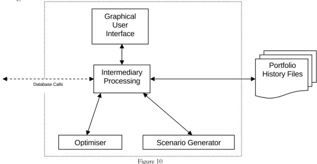
Figure 10 Database Calls Scenario Generator Optimiser Intermediary Processing Portfolio History Files Graphical User Interface

Graphical User Interface Intermediary Processing Scenario Generator Optimiser User will either

enter parameters through the interface or they will be imported from a file

2: Generate Scenarios

2.1: Generate Scenarios

2.2: Return Generated Scenarios 2.3: Display Scenarios

2.4: Optimise Portfolio

2.5: Return Optimised Portfolio 2.6: Display Optimised Portfolio

1: Obtain Portfolio Parameters

Figure 11

4.3 Graphical User Interface

As per the Specification, the Graphical User Interface needs to provide the user with a way to easily input the portfolio parameters and also display the outputs of the scenario generation and portfolio optimisation. Although there will be a large amount of data to display on the screen, not all of it will need to be viewable at the same time. For this reason, I will use a tabbed window structure to ensure that the user is not overwhelmed with information, but at the same time all of it will be easily accessible.

Figure 12 describes the overall structure of the application interface and has the portfolio parameters panel visible, highlighted in red. The annotations describe how the interface meets particular usability heuristics stated in [16].

status bar menu bar

portfolio scenario tree optimised portfolio portfolio history historical asset prices back-testing

Asset A

Load Portfolio Optimise Portfolio

Asset B Asset C Asset D Parameter A Parameter B Parameter C Parameter D (1) "Visibility of System Status" (8) "Aesthetic Minimalist Design" (2,4,6) "Match Between System

and Real World"; "Recognition Rather than Recall"; "Consistency" of terms

(5) Verification of inputs for "Error Prevention"

(7) Multiple methods of entering portfolio details allows for "Flexibility and Efficiency of Use"

Figure 12

The details of the future scenarios and final portfolio optimisation will be displayed in a similar way. By drawing out the scenario tree visually, the user will find it easier to assimilate the displayed data. As can be seen from the figure below, I intend to design the interface such that tree is displayed on the left of the window, and by clicking on the individual nodes of it, the details of either asset prices or optimised portfolio weights can be viewed.

Chapter 5

System Implementation

5.1 Implementation Languages

The implementation requirements stated in the Specification, lends itself to a two-tiered system. A high-level language will be able to provide a good graphical user interface but will be slow to perform the back-end portfolio optimisation calculations. Conversely, since a lower-level language is closer related to assembly language, it will be able to compute the portfolio optimisation faster, but lack the ability to provide the user with an easy to use graphical interface.

Figure 14 from [2] can be used as an example to quantifiably compare the speeds of common high and low level languages. It displays the normalised speeds for sparse matrix multiplication with various matrices on a Pentium 1.5GHz PC running a Linux Operating System.

Figure 14

I have made the assumption that this is the minimum specification of a typical user’s PC. Making use of its wide range of libraries, I have implemented the User Interface and intermediary processing in Java, a high level language. In order for the optimisation procedure to complete as quickly as possible I have implemented the numerical computation functions in FORTRAN, a low level language.

5.2 The Database

5.2.1 Database Implementation

In my system, the database is an integral component. It forms the core of the application, holding all of the historical financial data and statistical parameters for the optimisation procedure. The database will be a very active component of the system and will have a high throughput of data. The database has thus been designed in a way such that it is able to provide the facility to efficiently store the information as well as quickly retrieve it.

I considered the following options when deciding how to implement the database:

ƒ Native XML database

ƒ OLAP cubes

ƒ Relational database

Since the database will be storing financial information which I am downloading from an external source, I considered storing the data in an XML format. This would be a good option if the financial data I am downloading is also in an XML format since no conversion of format would be required for the downloaded data. However, searching the database will be problematic. Maintaining and using index documents would bear a large overhead. In addition, when search results are to be passed back to the client machine, entire XML documents may be sent back, even though only a few attributes from each are required. This will lead to an excessive volume of data being transferred between the database server and client machine and extra processing will be required in order to extract the required data from the XML documents returned; which will increase the time it takes to perform a database query.

OLAP functionality is characterised by its multi-dimensional data model. Since my database will be storing a large quantity of data, searching it could potentially be very slow. OLAP cubes overcome this by taking snapshots of a relational database and restructuring it into multi-dimensional data. Queries can then be run against this at a fraction of the time of the same query on a relational database, since their execution effectively returns the intersection of the required attributes. The difficulty in implementing OLAP comes in formulating the queries, choosing the base data and developing the schema.

Implementing the database in a relational format will give it a concise structure that can be easily queried. As long as it is normalised there will be no redundant data in the database, and hence keep the data consistent and the size of the database low. It is also beneficial that queries can be constructed easily in SQL to interrogate the relational database. For these reasons I decided to implement my database in a relational format.

5.2.2 Database Structure

A relational database follows the relational model which states that data is represented as mathematical n-ary relations. The following Entity Relationship diagram describes the structure of the tables that exist within my database.

symbol_table price_history constraints covariance has_ covariance N:1 1:N prices_for 1:N N:1 company_symbol: varchar period: integer value: decimal (10,10) company_name: varchar symbol: varchar trade_date: date price: decimal (10,2) symbol: varchar symboly: varchar symbolx: varchar trans_cost: decimal (10,10) has_ constraints 1:1 1:1 growth symbol: varchar growth_rate: decimal (10,10) period: integer has_ growth_rate N:1 1:N Figure 15

As can be seen from the diagram, the database is in third normal form since every non-prime attribute of each relation is:

ƒ Fully functionally dependent on every key of the relation. ƒ Non-transitively dependent on every key of the relation.

Having the database normalised means that it is not possible to create data inconsistencies when adding, deleting and modifying data. It also means that no repetitive data is being stored, reducing the size of the overall database.

While implementing the database I wanted to maintain un-biased database structures as I feel that both reading from and writing to the database are equally important. For example, when calculating the covariance matrix for all of the assets within the system, it needs to parse through all of the historical price data to perform the calculation and then store the results back to the database. This task consists of high volumes of data being transferred both out of and into the database.

In order to achieve increased performance I have created SQL constraints on the tables. By enforcing primary keys on the database tables, the database management system (DBMS) implicitly creates an index structure on the key fields. This allows for the quick retrieval of data from the table if the data is being queried on the key. However, if I was to query the data using a non-key field, the DBMS retrieves data by performing a scan of the whole table. This clearly increases the time it takes for data to be returned.

By adding further indexes onto the table, data can be returned for queries using other fields by using these indexes, eliminating the need to scan through the whole table and thus decreasing the time it takes for them to run. However, in contrast, when writing data to a table with several indexes the DBMS must update each of the indexes, which obviously takes longer to perform when more indexes exist. Therefore, a balance needs to be achieved when deciding upon the number of indexes to attach to each table.

For my database, I have setup primary keys as stated in the above diagram. By analysing the queries I am running on the database, further described in Section 5.2.3, I discovered that all queries were using these fields and hence, these were the only indexes required for each table. In order to ensure data consistency in my database, I also created foreign key constraints on attributes of tables wherever required. This ensures that any manipulation of data is always consistent and no anomalous data can ever be stored.

5.2.3 Database API

Since the database is accessed by several different components of the system, I decided that it would be advantageous if it could be encapsulated by an API. This will ensure that other components can not illegally access the database and so that standardised results can be returned. I have implemented the API in two tiers:

ƒ Stored Procedures ƒ Java API Class

A stored procedure is a program which is physically stored within a database. One benefit this provides is pre-compilation. When a stored procedure is created the query plan is calculated once, rather than every time the query is submitted. This removes the ad-hoc SQL compilation overhead that is required in situations where actual SQL queries are piped to the database. Having stored procedures will therefore mean that queries can be executed faster. Stored procedures also allow the underlying tables to be encapsulated. From a security point of view, this means that access to the database is only allowed through narrow, well-defined procedures. Rather than having the other application components interact with the tables and other database objects directly, they will only be allowed to run the stored procedures.

As mentioned in Section 5.2.2, I conducted analysis of whether I needed to create any extra indexes on the tables in the database. To do this, I formulated a list of the representations of the stored procedures which search for data using relational algebra. This allowed me to see which fields are being used in my queries, and analyse whether any do not have an index on them. Appendix Section A contains a list of the stored procedures in my database and their relational algebra representation. As can be seen from the list, the stored procedures only contain select clauses on primary key fields of the tables; which is why I did not add any further indexes to them.

On top of the stored procedures I have written a Java API class which manages the connection of the application to the database server and also provides an interface to access the database. Each stored procedure stated in the list is accessible through its respective function in the API. Rather than simply return an abstract object result set, the API returns an object of the same data type as the underlying data. This eliminates the need for other components to parse the data being returned by the database and convert it into the required data-type.

I have implemented the database API as a singleton class to ensure that the client application only makes at the most one connection to the database server. This means that it will not be swamped by several connections from the same machine all requesting high throughput. Although I have not had to, having a singleton class also means that I could restrict the number of concurrent database calls the application makes, which could be used to avoid creating too much network traffic or to control the load on the database server.

5.3 The Data Downloader

5.3.1 Data Source

The historical prices of assets in the database form the underlying basis for the scenario generation and hence the optimisation procedure. Since I intend Portfolio Managers using my application to be interested in making long-term capital gains, I will only need to acquire close of day prices and not intra-day prices. I have stated in my Specification that I will include assets from FTSE 100 in my database. A free source of this data is “Yahoo! Finance UK”. They make available a comma separated value (.csv) file which contains the latest prices of all of the components of the FTSE 100 exchange. This file can be downloaded over the internet via the URL:

http://uk.old.finance.yahoo.com/d/quotes.csv?s=@%5EFTSE&f=sl1d1t1c1ohgv&e=.csv

5.3.2 Data Acquisition

In order to download the data and insert it into the database, the following class structure was written: -downloadData() -updateGrowthRate() -updateCoVar() Main +covariance() +growthRate() Statistics -connect(in url : string)

+download()

-parseLine(in line : string) -readLine() : string

Downloader

+insertAssetPrice(in asset : string, in date : string, in price : double)

+setCovariance(in assetX : string, in assetY : string, in covariance : double, in period : int) +getPrices(in asset : string, in period : int) : double[]

+setGrowth(in asset : string, in growthRate : double, in intercept : double, in period : int) +getAllAssets() : string[][] JDBC 1 1 1 1 Figure 16

The Main class initiates the downloading of data, after which it instantiates the Statistics class to perform the updating of the parameters. All three classes reference the singleton database API in order to insert and update data.

5.3.3 Parameters Re-calculation

As is described in further detail in Section 5.4, in order to generate future scenarios, the Scenario Generator requires values for the growth rate and covariance of assets from the mean exponential growth curve. Once a new set of prices have been calculated, these values need to be recalculated. For this reason, I have included this process as part of the Data Downloader module. Once the new price data has been downloaded, the module performs the recalculation of the parameters and stores them in the database.

5.3.4 Job Automation

The downloading of prices and re-calculation of parameters is a task which will need to be done at the close of every day. Since this a menial task that does not require any human interaction, it lends itself to be fully automated. Having the job automated also means that when users wish to optimise a portfolio they can be sure that the latest price data and parameters have already been calculated, speeding up the whole optimisation process.

With the help of Duncan White, from CSG, a CRON was set up to run at 19:00 every weekday. The job runs a batch script in my user space which in-turn executes the compiled Java Data Downloader package.

5.4 The Scenario Generator

5.4.1 Cluster

To generate the future scenarios I will be using Cluster, introduced in my Background Research. I did not have access to the source of the program so the only method of executing it was through the command line. This is not the ideal way, since it would be quicker to be able to call the Cluster method and directly pass parameters to it via memory. By having to output the inputs to a file and then parse the output file to place the outputs back into memory, the overall execution time will increase since it is slower to perform file I/O rather than memory I/O.

Cluster requires as input a file with the following structure: