Author(s) Shieh, AD; Hung, YS
Citation Statistical Applications In Genetics And Molecular Biology, 2009,v. 8 n. 1, article no. 13
Issued Date 2009
URL http://hdl.handle.net/10722/58817
Albert D. Shieh and Yeung Sam Hung
Abstract
In this paper, we address the problem of detecting outlier samples with highly different expression patterns in microarray data. Although outliers are not common, they appear even in widely used benchmark data sets and can negatively affect microarray data analysis. It is important to identify outliers in order to explore underlying experimental or biological problems and remove erroneous data. We propose an outlier detection method based on principal component analysis (PCA) and robust estimation of Mahalanobis distances that is fully automatic. We demonstrate that our outlier detection method identifies biologically significant outliers with high accuracy and that outlier removal improves the prediction accuracy of classifiers. Our outlier detection method is closely related to existing robust PCA methods, so we compare our outlier detection method to a prominent robust PCA method.
Author Notes: The authors would like to thank the anonymous reviewers, whose comments helped improve the manuscript.
1
Introduction
Microarray data contains gene expression levels for a number of samples, each of which is labeled with a biological class, such as a tumor type or an experimental condition. There is a large body of methods for the analysis and interpretation of microarray data, particularly for the problems of gene selection and class prediction. However, an issue that has not been thoroughly studied is how to deal with outlier samples. We define an outlier as a sample that deviates significantly from the rest of the samples in its class. The practical consequence of designating a sample as an outlier is that its class membership must be called into question since the sample appears to have been generated by a different process. There is an enormous amount of literature on outlier detection (Barnett and Lewis, 1994), but few outlier detection methods have been proposed for the noisy, high dimensional, and class labeled nature of microarray data.
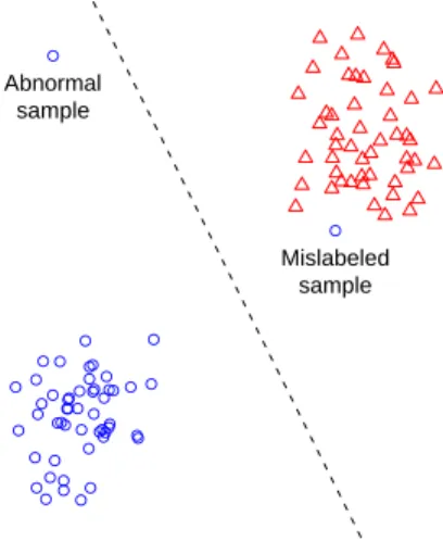
There are two main types of outliers in microarray data. The first type of outlier is a sample that belongs to a different class present in the data, which are often re-ferred to as mislabeled samples. These are samples that were incorrectly assigned to a class, such as a tumor sample that was labeled as a normal sample. These out-liers are commonly discovered by classification methods, which will consistently misclassify the outliers to their true class. The second type of outlier is a sample that does not belong to any class present in the data, which we will refer to as abnor-mal samples. The source of these outliers is more ambiguous, but they can result from an undiscovered biological class, poor class definitions, experimental error, or extreme biological variability. Note that when we say an abnormal sample does not belong to its class, we are not necessarily contesting the validity of its label. For example, a sample may truly be a tumor, but have expression levels that differ greatly from those of other tumor samples. The sample should still be treated as an outlier since it does not follow the expression pattern of its class. Examples of the two types of outliers are shown in Figure 1.
It is important to separate outliers in microarray data analysis since they are in-consistent with the rest of the data and, in the case of mislabeled samples, may even contain incorrect biological information. Applying models to data in the presence of outliers can produce skewed parameter estimates and even incorrect inferences. However, the influence of outliers is rarely considered in standard microarray data analysis. Outliers are probably ignored in practice because of their low prevalence. Microarray experiments can be carried out precisely, so many sources of error that can create outliers are eliminated. Additionally, samples with measurements that deviate significantly are often screened out as a part of experimental procedure. However, outliers caused by biological factors that cannot be controlled for do oc-cur often enough to warrant attention. For example, the colon cancer data set (Alon
● ● ● ● ● ● ● ● ● ● ● ● ● ●● ● ● ● ● ● ● ● ● ● ● ● ● ● ● ● ● ● ● ● ● ● ● ● ● ● ● ● ● ● ● ● ● ● ● ● ● Mislabeled sample ● Abnormal sample
Figure 1: Examples of the two types of outliers.
et. al., 1999), one of the most widely used benchmark data sets, is known to contain several samples that are either contaminated or mislabeled (Li et. al., 2001) because of the difficulty of collecting clean tumor samples. These samples are reported to have an adverse effect on the prediction accuracy of classification methods and are often removed from the data set.
We believe that a formal method of dealing with outliers is needed as a data quality check. Most of the methods currently used in microarray data analysis are not robust to outliers. Although robust methods are being developed, it is practical to consider the detection of outliers as a separate problem. An outlier detection method can be used as a preprocessing step before applying current non-robust methods. Once outliers are identified, they can be examined by the experimenter and dealt with appropriately depending on the type of outlier and problem under consideration. If outliers correspond to biological anomalies, then they may be of further substantive interest to the experimenter. If outliers correspond to mislabeled samples, then the experimenter may be able to correct the class labels. In problems such as class prediction, it may be advantageous to remove or weight outliers in classifiers in order to decrease their influence on the decision boundary (Li et. al., 2001). However, it is important to emphasize that, in many cases, outliers may simply be the result of natural variability in the data (Barnett and Lewis, 1994). Samples that lie in the tails of the data distribution are still valid samples and it can be particularly easy to identify these samples as outliers with the small sample sizes of microarray data. We highly discourage against casually discarding samples on the basis that they are outliers without a more substantive explanation, such as sample contamination. Outlier detection should be treated as one of many tools for
the experimenter to evaluate data quality, but should never be treated as definitive or a substitute for careful examination by the experimenter.
Outlier detection in microarray data is complicated by the presence of class in-formation. Rather than finding outliers with respect to the data, the problem is to find outliers with respect to each class. A mislabeled sample is not an outlier in the data, but it is an outlier in its class. It may seem that outlier detection is simply a classification problem where consistently misclassified samples must be identified. In this case, any classifier can be applied using cross-validation to find misclassified samples. Outlier detection has been addressed in a limited context as it relates to class prediction. Furey et. al. (2000) and Moler et. al. (2000) proposed similar methods using leave-one-out cross-validation (LOOCV) with a linear support vec-tor machine (SVM) classifier. Li et. al. (2001) proposed using a genetic algorithm with ak-nearest neighbor (k-NN) classifier. These methods were all applied to the colon cancer data set and found outliers consistent with those originally reported in Alon et. al. (1999). However, classification methods cannot truly solve the out-lier detection problem because they can only find mislabeled samples that can be discriminated by the class label, but not abnormal samples that come from an un-known class. Baty et. al. (2008) proposed a more general method using jackknife resampling to test the instability of samples in a between-group analysis (BGA). Samples that are significantly influential towards the positions of other samples are deemed outliers. Although this method is theoretically capable of identifying abnormal samples, it relies heavily on a data representation constructed from all classes. This method was tested against three data sets of varying heterogeneity, but there were no known outliers to validate the method against. To our knowledge, these are the only significant methods that have been proposed for outlier detection in the microarray literature.
Existing outlier detection methods based primarily on using class information to separate the samples into groups assume that the data are fairly well behaved. If classes are not separable or the data are highly heterogeneous, it is likely that false positives, or inlier samples mistaken for outlier samples, will be identified. For example, outlier detection methods based on cross-validation of a classifier need perfect prediction accuracy from the classifier in order to avoid producing false positives. Additionally, existing methods rely on computationally intensive resam-pling procedures that are costly for a preprocessing task such as outlier detection. Most importantly, none of the existing methods have been validated extensively. Existing methods have been tested on individual data sets and the results have been qualitatively interpreted, but no attempt has been made to estimate the general ac-curacy of these methods. This is largely due to a difficult methodological issue of how to obtain known outliers to validate against. However, without knowing the general accuracy of an outlier detection method, it is dubious to suggest its usage.
We propose to ignore other classes for outlier detection and instead treat each class as a separate data set. The goal of outlier detection is to capture the content of each class and separate it from all other possible classes, which are outliers. Under this framework, mislabeled and abnormal samples are effectively treated the same way since they both belong to some unknown class.
In this paper, we propose a simple, automatic outlier detection method suitable for microarray data that treats each class independently and uses a statistically prin-cipled threshold for outliers. Our outlier detection method is able to detect both mislabeled and abnormal samples without reference to other classes. We demon-strate the performance of our outlier detection method in three ways. First, we apply our outlier detection method to two widely used data sets in order to validate that biologically meaningful outliers are identified. Second, we demonstrate that outlier removal can improve the prediction accuracy of several common classifiers. Finally, we estimate the accuracy of our outlier detection method by simulating new data sets where outliers are introduced from unobserved classes. Our outlier detection method bears many similarities to robust principal component analysis (ROBPCA), a prominent outlier detection method in the chemometrics literature (Hubert et. al., 2005), which also frequently deals with high dimensional data, although usually on a lower scale. Therefore, we evaluate the suitability of ROBPCA for microarray data in comparison to our outlier detection method.
2
Methods
2.1
Dimension reduction
Microarray data contains a large number of genes p, usually in the thousands to tens of thousands, compared to the number of experimentsn, usually in the tens to hundreds, making the direct application of standard multivariate analysis methods impossible. Particularly, most outlier detection methods rely on computing some type of distance function for each sample. However, in high dimensions, the data becomes sparse and distances become effectively meaningless. Therefore, the di-mension of the data must be reduced before outlier detection methods based on distances can be applied. There are some outlier detection methods based on pro-jection pursuit that can inherently handle the high dimensionality of microarray data. These methods try to find projections of the data onto lower dimensional subspaces where outliers are easy to identify and have been applied successfully to finding outlier genes, or informative genes (Filzmoser et. al., 2008). However, we found that these methods did not work well when applied to detecting outlier samples. Only a small number of the genes in microarray data are informative and
the rest of the genes are effectively noise. Projecting the data onto a set of genes that are not informative may produce a subspace that separates samples well, but is biologically meaningless. In practice, we found that methods based on projection pursuit are prone to false positives and are highly sensitive to small changes in the data. Therefore, we will focus on an outlier detection method based on distances coupled with a dimension reduction method.
Dimension reduction methods for microarray data can be divided in two ways, gene selection or feature extraction and supervised or unsupervised. Gene selection finds a subset of genes and is usually supervised, while feature extraction constructs new components and is either supervised or unsupervised. Since we want to treat each class independently in our outlier detection method and avoid overfitting our data representation to the class labels (Khan et. al., 2001), we will only consider unsupervised dimension reduction methods. The most widely used unsupervised feature extraction method is principal component analysis (PCA). Consider a data matrix X with n experiments in rows and p genes in columns. Classical PCA projects the data ontonprincipal components, or linear combinations of genes
wi =Xvi (1)
that maximize the variance
vi = arg max
v0v=1Var(Xv) (2)
subject to the constraint of orthogonality Cov(wi,wj) = 0 for all j < i where
i, j = 1, . . . , n. The principal components are ordered by how much of the variance in the data that they explain. It is well known that PCA itself is not robust to outliers (Hubert et. al., 2005). However, we are only using PCA to reduce the dimension of the data, not to find a robust data representation.
Althoughnprincipal components are produced, usually only a small number of
m < nprincipal components are needed to explain most of the variance in the data. Selecting the optimal number of principal components is difficult since selecting too many results in unnecessary complexity, while selecting too few results in a loss of information. One of the most widely used methods in practice is examining a scree plot of the ordered variances d1, . . . , dn of the principal components and searching for an elbow point where the amount of additional variance explained by adding another principal component drops off sharply (Hastie et. al., 2001). Since examination of the scree plot is difficult and subjective, we use an automatic selection method based on the scree plot (Zhu and Ghodsi, 2006). The automatic selection method assumes that the distribution of the variances changes at the elbow point m and the variances D1,m = (d1, . . . , dm) and D2,m = (dm+1, . . . , dn) are
normally distributed. The elbow pointm can be found by maximizing the profile log-likelihood function L(m) = m X i=1 logN(di|θˆ1,m) + n X j=m+1 logN(dj|θˆ2,m) (3)
whereN denotes the normal density andθˆ1,mandθˆ2,mare the maximum likelihood estimates forD1,mandD2,mwith pooled variance. The automatic selection method is fast and has been shown to perform well on various types of high dimensional data (Zhu and Ghodsi, 2006).
2.2
Outlier detection
Since each class in a data set has a different underlying distribution, we treat each class as an independent data set for the purpose of outlier detection. Consider a class containingn samplesxi, i = 1, . . . , nwith pprincipal components, for which we will assume p < n. Statistical methods of outlier detection compute the distance of each sample from the center of the data and identify samples above a certain threshold as outliers. The classical measure of the outlyingness of a sample xi is the Mahalanobis distance
d(xi) = p
(xi−t)0C−1(x−t) (4) where t and C are the sample mean and covariance. However, it is well known that the sample mean and covariance are highly susceptible to outliers. Although Mahalanobis distances can detect single outliers, they breakdown in the presence of multiple outliers due to the masking effect, where multiple outliers will not all have large Mahalanobis distances (Rousseeuw and Leroy, 1986). Therefore, it is neces-sary to use a robust version of the Mahalanobis distance, which is often referred to as the robust distance, using robust estimates of the mean and covariance. The two problems associated with outlier detection are then obtaining robust estimates of the meantand covarianceCand determining a threshold for the robust distance
d(xi)above which a samplexi should be identified as an outlier.
First, we address the issue of robust estimation. Robust estimators aim to achieve a high breakdown point, or proportion of the data that can be outliers before the estimates become unreliable, while maintaining high efficiency. Additionally, since PCA is used for dimension reduction, robust estimators must be equivariant under orthogonal transformations. Many robust estimators with good theoretical properties have been proposed, but two of the most commonly used robust estima-tors are the minimum volume ellipsoid (MVE) and minimum covariance determi-nant (MCD) estimators (Rousseeuw, 1985). The MVE estimator sets the mean t
and covarianceCto the center and ellipsoid of the minimum volume ellipsoid con-tainingh < n samples. The MCD estimator sets the meant and covarianceCto the sample mean and covariance ofh < nsamples for which the determinant of the sample covariance is minimum. Whenh =b(n+p+ 1)/2c, the MVE and MCD estimators can achieve the optimal breakdown point of b(n−p+ 1)/2c/n. How-ever, the MVE and MCD estimators have low efficiency whenh is selected for a high breakdown point. Additionally, in practice the MVE and MCD estimators are prone to false positives with small sample sizes, which are common in microarray data, and the resampling algorithms used to compute the MVE and MCD estimators can produce unstable results (Ruppert, 1992).
A more powerful class of robust estimators closely related to the MVE and MCD estimators is the S-estimator (Davies, 1987). The S-estimator finds vectort
and positive definite symmetric matrixCthat minimizedet(C)subject to 1 n n X i=1 ρ(d(xi)) =b0 (5)
whereρis a nondecreasing function on[0,∞)andb0is a constant that controls the breakdown point. The function ρ is usually also differentiable, but the MVE and MCD estimators can be seen as special cases of S-estimators where the functionρ
is 0 or 1. The functionρmust be bounded in order to obtain a nonzero breakdown point. The ratio of the constant b0 to the maximum of the function ρ defines the breakdown point. The function ρ is usually specified in terms of a base function
ρ0, which obtains its maximum atc0, scaled by a constantc, which varies with the dimensionp. The constraint (5) can then be rewritten as
1 n n X i=1 ρ(d(xi)/c) =b0 (6)
where the constantsb0 andcare chosen such thatE(ρ(d/c)) = b0 andb0 =rρ(c0) for a breakdown point of r. We use the optimal breakdown point of r = 0.5 in our S-estimator. Although some efficiency must be sacrificed in order to obtain the optimal breakdown point, using a high breakdown point is known to work well in practice (Rocke, 1996) since it decreases the weight given to outliers. When specifying the functionρ, it is usually easier to work withψ =∂ρ/∂dsinceψ has a root whereρhas a minimum. We use the standard Tukey’s biweight function
(y) = (
y(1−(y/c0)2)2 if|y|< c0
0 if|y|> c0
(7) which is a redescending function with support[−c0, c0]. Tukey’s biweight function is known to work well because it behaves similarly to the squared error function
for small to moderate deviations, allowing it to achieve high efficiency, but tapers off for large deviations, allowing it to decrease the weight given to outliers. It is worth noting that the S-estimator is highly efficient at multivariate normal models, an assumption that we will use later (Rocke, 1996).
Solving the minimization problem for the S-estimator exactly involves a large combinatorial search that is computationally intractable. Therefore, a resampling algorithm that reduces the number of times the objective function is evaluated must be used. We use a modification of the fast-S algorithm (Salibian-Barrera and Yohai, 2006), an improvement on the SURREAL algorithm (Ruppert, 1992), originally intended for S-estimators of regression. We use the implementation of the fast-S algorithm in the R package rrcov. It is important to note that robust estimators become unreliable for small sample sizes, especially when n < 2p, because the weighting of each sample becomes highly influential towards the estimates. Sample sizes this small do occur occasionally in microarray data sets, usually when there are many classes present. We propose using the sample mean and covariance instead of the S-estimator when the sample size approachesn <2p.
Now, we address the issue of explicitly identifying outliers. The distribution of the robust distances must be known in order to determine a threshold at which to reject samples as outliers, which usually entails making an assumption about the distribution of the data. If the data follows a multivariate normal distribution, then the squared robust distancesd2(x
i)will approximately follow aχ2distribution with
p degrees of freedom (Rousseeuw, 1987). Under this assumption, an appropriate cutoff value for outliers is the standard 97.5% quantile of theχ2distribution withp degrees of freedom, which we will denote asχ2
p,0.975. There are more sophisticated methods for determining a threshold using other distributions (Hardin and Rocke, 2005), but the simpleχ2
p,0.975threshold is known to perform well in practice (Hubert et. al., 2005). It is worth noting that there is a2.5%chance that theχ2
p,0.975threshold will identify a sample as an outlier, even if there are no outliers. However, we prefer to identify all of the outliers at the risk of accidentally identifying a small number of inliers as outliers.
Our outlier detection method can be thought of as fitting an ellipsoid to the good part of the data and excluding all samples outside of the ellipsoid as outliers. The shape of the ellipsoid is determined by the robust estimates and threshold. Our outlier detection method contains three hyperparameters, the number of principal components, the breakdown point, and the distance threshold. However, none of the hyperparameters need to be specified by the experimenter. The number of principal components is determined using an automatic selection method to find the elbow point of the scree plot, while both the breakdown point and the distance threshold are fixed in accordance with widely used values in the outlier detection literature (Rocke, 1996; Rousseeuw, 1987).
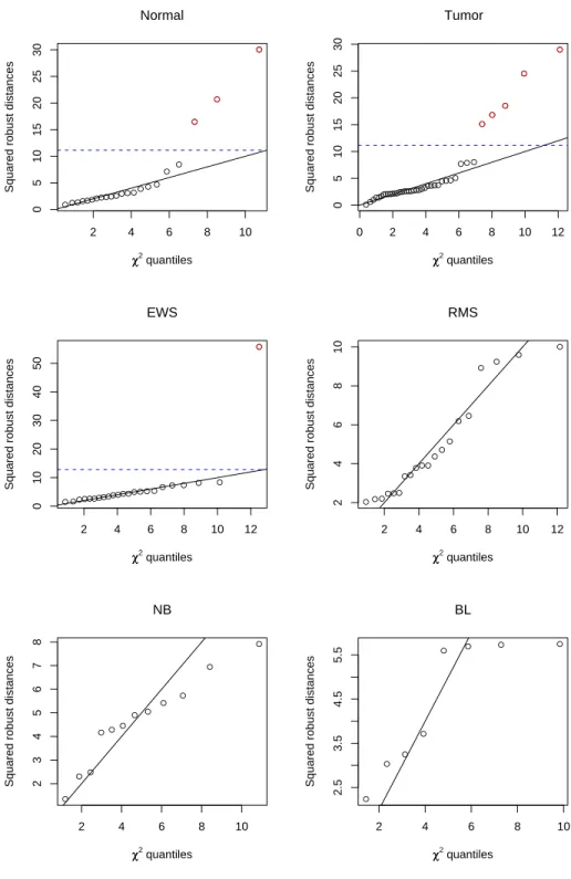
It may seem that the normality assumption is too strong for microarray data, which is thought to be extremely complex. However, many commonly used para-metric methods, such as the t-statistic for gene selection and linear discriminant analysis (LDA) for class prediction, also make a normality assumption and have been shown to have good performance empirically (Dudoit, 2002). We found that the normality assumption is reasonable for the purpose of outlier detection when proper preprocessing is performed. In raw microarray data, the variance of the ex-pression levels usually increases linearly with the mean of the exex-pression levels, resulting in an asymmetric distribution with a long tail towards high expression lev-els. Therefore, a variance stabilizing transformation is necessary in order to make the variance more constant and the distribution more symmetric. We use a base-2 logarithm transformation and quantile normalization, as recommended by Bolstad et. al. (2003). A graphical method of testing the normality assumption is to con-struct a quantile-quantile plot of the observed squared robust distances against the theoreticalχ2quantiles. If the normality assumption is correct, then the data should follow a straight line, except for the outliers. If the data deviates significantly from a straight line, then our outlier detection method will become unreliable.
2.3
ROBPCA
Our outlier detection method is similar to a number of robust PCA methods in the chemometrics literature (Egan and Morgan, 1998; Hubert et. al., 2002) that can be used to identify outliers in high dimensional data, the most promiment of which is ROBPCA (Hubert et. al., 2005). ROBPCA has also been applied to some types of biological data with fewer dimensions than microarray data, such as nuclear magnetic resonance (NMR) spectroscopy data and reverse transcription polymerase chain reaction (RT-PCR) data (Hubert and Engelen, 2004). However, microarray data is different from other high dimensional data because a large number of the genes are not informative, so many of the dimensions are effectively meaningless. Therefore, as we discussed earlier, most of the subspaces in microarray data cannot be used for methods such as projection pursuit.
ROBPCA fits a robust PCA space to the data using a combination of projection pursuit and robust estimation methods. First, a projection pursuit step is used to find a subset of the least outlying samples to construct a preliminary robust PCA space. Then, a robust estimation step is used on the preliminary robust PCA space to construct a refined robust PCA space. Two types of distances are used to identify outliers in the robust PCA space. A score distance, which is identical to our robust distance, is used to measure how far a sample is from the center of the data in the robust PCA space and an orthogonal distance is used to measure how far a sample is from the robust PCA space in the original data space. An orthogonal distance
is needed to incorporate outliers that were excluded in the projection pursuit step from constructing the robust PCA space. Our outlier detection method does not use an orthogonal distance since a classical PCA space including outliers is used. The score distance threshold uses aχ2 distribution, which is identical to our robust distance threshold, and the orthogonal distance threshold uses an adaptively scaled
χ2 distribution.
ROBPCA can be applied to data with class labels in two ways. The simplest method is to disregard the class labels and apply ROBPCA to fit a single robust PCA space to all of the classes (Hubert et. al., 2004). A more flexible method is to treat each class independently and apply ROBPCA to fit a different robust PCA space to each class (Vanden Branden and Hubert, 2005). On the other hand, our outlier detection method fits a single classical PCA space to all of the classes, but uses robust estimation on each class independently. Our outlier detection method is able to compromise between incorporating information from all classes and treating each class independently because classical PCA and robust estimation are separate steps. The main differences between ROBPCA and our outlier detection method are that ROBPCA uses projection pursuit and robust estimation in robust PCA for both dimension reduction and outlier detection, while our outlier detection method uses classical PCA for dimension reduction and robust estimation for outlier detection.
3
Results
3.1
Data sets
We tested our outlier detection method on two widely used benchmark data sets: • The colon cancer data set (Alon et. al., 1999) contains 62 samples, of which
22 samples are from normal tissue and 40 samples are from tumor tissue. Expression levels for more than 6,500 genes were measured using Affymetrix oligonucleotide arrays. The data set was filtered down to the 2,000 genes with the highest minimal intensity across all of the samples.
• The small, round blue cell tumor (SRBCT) data set (Khan et. al., 2001) contains 63 samples, of which 23 samples are from the Ewing family of tu-mors (EWS), 20 samples are from rhabdomyosarcoma (RMS), 12 samples are from neuroblastoma (NB), and 8 samples are from Burkitt lymphoma (BL). Expression levels for 6,567 genes were measured using glass slide cDNA mi-croarrays. The data set was filtered down to the 2,308 genes with sufficient red intensity across all of the samples.
We applied a base-2 logarithm transformation and quantile normalization to both data sets. No scaling was applied to the genes or the samples since we do not want to treat inliner and outlier samples or informative and non-informative genes equally. We chose one data set with two classes and one data set with multiple classes in order to demonstrate that our outlier detection method performs well regardless of the number of classes present in the data set. Additionally, we chose two data sets with heterogeneity in order to demonstrate that our outlier detection method performs well on classes with complex structure. The colon cancer data set is heterogeneous because the tissue samples contain a mixture of cell types. The SRBCT data set is heterogeneous because the samples came from both tumor biopsy material and cell lines. The colon cancer and SRBCT data sets are amongst the more difficult benchmark data sets to achieve good prediction accuracy on (Lee et. al., 2005), so they should be challenging for outlier detection.
3.2
Detection of known outliers
We applied our outlier detection method to the colon cancer and SRBCT data sets, treating each class independently. Four principal components were chosen for the colon cancer data set and five principal components were chosen for the SRBCT data set using the automatic selection method. Scree plots for each data set are shown in Figure 2. The black bars denote the selected principal components and the grey bars denote the remaining principal components. Since the NB and BL classes had small sample sizes, the sample mean and covariance were used instead of the S-estimator for computing the robust distances. The normality assumption held well on both the colon cancer and SRBCT data sets. Quantile-quantile plots for each class are shown in Figure 3. The blue, dotted lines denote the χ2
5,0.975 threshold for outliers and the red points above the threshold denote the identified outliers. The solid line with unit slope denotes the expected pattern for the samples if the normality assumption holds. The linear fit was generally good, especially for the tumor, normal, EWS, and RMS classes. The NB and BL classes did not fit the line as well, but their deviation can likely be attributed to their small sample sizes. For sufficiently large sample sizes, the quantile-quantile plots indicate that the normality assumption works well, even on highly heterogeneous data.
First, we address the colon cancer data set. Several classification methods have been applied to the colon cancer data set and have found consistently misclassified samples, which have been declared to be outliers in the literature. Misclassified samples are not always outliers since they can result from problems in the classifier used rather than inherent properties of samples. However, examination of the tissue composition of the misclassified samples has revealed substantial differences that support their identification as outliers. We will validate our outlier detection method
Colon cancer Principal components Variance 0 50 100 150 SRBCT Principal components Variance 0 50 100 150 200 250
Figure 2: Scree plots for the colon cancer and SRBCT data sets.
against these known outliers. In the original analysis of the colon cancer data set, Alon et. al. (1999) used a two-way clustering algorithm based on deterministic annealing and found that eight samples were misclassified (T2, T30, T33, T36, T37, N8, N12, and N34). Furey et. al. (2000) and Moler et. al. (2001) used similar linear SVM classifiers with LOOCV and found that six samples were misclassified (T30, T33, T36, N8, N34, and N36). In two separate analyses, Li et. al. (2001) used a genetic algorithm with a k-NN classifier and found that six samples were misclassified (T30, T33, T36, N8, N34, and N36). Overall, there are nine samples that have been reported as outliers (T2, T30, T33, T36, T37, N8, N12, N34, and N36).
The outliers in the colon cancer data set are suspected to be caused by high heterogeneity in the tissue composition. Alon et. al. (1999) computed a muscle index, a measure of the muscle content of a sample based on genes relevant to smooth muscle, for each sample. Normal samples consist of a mixture of cell types, while tumor samples consist of mostly cancerous epithelial cells. Therefore, normal samples should have high muscle index and tumor samples should have low muscle index. However, the outlier tumor samples (T2, T30, T33, T36, and T37) have high muscle index and the outlier normal samples (N8, N12, N34, and N36) have low muscle index, suggesting that the tissues in the outlier samples are contaminated with other cell types. Li et. al. (2001) confirmed in communications that the outlier samples have a different tissue composition, particularly in the ratio of epithelial cells, from the rest of the samples in their respective classes. It is interesting that the outliers resemble samples from the opposite class. The outlier tumor samples have muscle index consistent with normal samples and the outlier normal samples
● ●●●●●● ●●●●●●● ● ●● ● ● ● ● ● 2 4 6 8 10 0 5 10 15 20 25 30 χχ2 quantiles
Squared robust distances
● ● ● Normal ●●●●● ●●●●●●●●●●●●●●●●●●●●● ●●●●●● ●● ● ● ● ● ● ● 0 2 4 6 8 10 12 0 5 10 15 20 25 30 χχ2 quantiles
Squared robust distances
● ● ● ● ● Tumor ● ●●●●●●●●●● ●●●● ● ●● ● ● ● ● ● 2 4 6 8 10 12 0 10 20 30 40 50 χχ2 quantiles
Squared robust distances
● EWS ● ● ● ●●● ●● ●●● ●● ● ●● ● ● ● ● 2 4 6 8 10 12 2 4 6 8 10 χχ2 quantiles
Squared robust distances
RMS ● ●● ● ●● ● ● ● ● ● ● 2 4 6 8 10 2 3 4 5 6 7 8 χχ2 quantiles
Squared robust distances
NB ● ● ● ● ● ● ● ● 2 4 6 8 10 2.5 3.5 4.5 5.5 χχ2 quantiles
Squared robust distances
BL
have muscle index consistent with tumor samples. It is unlikely that the outliers are mislabeled samples since they were closely examined in Alon et. al. (1999). However, we found that the primary reason that the outliers could be identified by classification methods was that the outliers were located on the opposite side of the decision boundary separating the classes.
Our outlier detection method found eight outlier samples (T2, T30, T33, T36, T37, N8, N34, and N36) corresponding to all of the reported outliers except for the sample N12. We examined the sample N12 and found that it may not be an outlier. Since the outlier samples are contaminated, they should be distinguished by their inconsistent muscle index. The muscle index for the normal samples excluding the outliers range from 0.3 to 1.0, while the muscle index for the outliers N8, N34, and N36 is below 0.2. However, the sample N12 has muscle index 0.4, which falls well within the range for normal samples. Additionally, we found that using a muscle index of 0.2 to 0.3 as a threshold to separate the classes identified all of the outliers except for the sample N12. Therefore, the sample N12 does not appear to be contaminated and it is reasonable to conclude that it is not an outlier. The sample N12 was only reported to be an outlier once in Alon et. al. (1999) and may have been misclassified because the classifier used was not optimal. Excluding the sample N12, our outlier detection method identified all of the outliers suspected to be contaminated.
Now, we address the SRBCT data set. There are no samples strictly known to be outliers in the SRBCT data set. However, in the original analysis of the SRBCT data set, Khan et. al. (2001) used a linear artificial neural network (ANN) classifier with resubstitution and found that all but one sample (EWS-T13) could be classified confidently. Although the sample EWS-T13 was assigned to the correct class, it fell below the confidence threshold proposed for accurate diagnosis. The confidence threshold is based on the distance of a sample from the ideal location of its class in the feature space, suggesting that the sample EWS-T13 lies far away from most of the samples in its class. Manually examining the samples in the EWS class using two standard data representation methods, multidimensional scaling (MDS) analysis as proposed in Khan, et. al. (2001) and BGA as proposed in Culhane et. al. (2002), confirmed that the sample EWS-T13 is highly distant from the rest of the samples in its class. Therefore, it is reasonable to identify the sample EWS-T13 as a outlier. The sample EWS-EWS-T13 seems to be an example of an abnormal sample that deviates from its class due to natural biological variability. We found that classification methods did not misclassify the sample EWS-T13 because it was located within the decision boundary for its class. Our outlier detection method identified the sample EWS-T13 as an outlier, demonstrating how it can identify all types of outliers.
3.3
Comparison to ROBPCA
We applied ROBPCA to the colon cancer and SRBCT data sets in order to evaluate the performance of ROBPCA on microarray data. We used the known outliers in the colon cancer and SRBCT data sets as a basis for comparison. We used the im-plementation of ROBPCA in the R package rrcov with default parameters. Fitting different robust PCA spaces to each class performed much better than fitting a sin-gle robust PCA space to all of the classes, so we treated each class independently. Diagnostic plots of the orthogonal and score distances for each class are shown in Figure 4. The blue, dotted lines denote the orthogonal and score distance thresh-olds, the red points denote true positives, and the filled points denote false positives. ROBPCA identifies at least a few outliers for each class, indicating that ROBPCA may be prone to identify too many outliers.
On the colon cancer data set, ROBPCA identified one false negative (T30) and 12 false positives (T5, T6, T9, T12, T19, T25, T29, T39, T40, N4, N8, N29). On the SRBCT data set, ROBPCA identified 17 false positives (EWS-T4, EWS-T6, EWS-T9, EWS-T19, EWS-C4, T1, T5, T7, T10, RMS-T11, RMS-C8, NB-C5, NB-C8, NB-C10, NB-C12, BL-C2, BL-C5). Although ROBPCA was able to identify almost all of the true positives, it also identified a large number of false positives. ROBPCA identified 19.4% of the samples in the colon cancer data set and 27.0% of the samples in the SRBCT data set as out-liers. The orthogonal distance appears to perform better than the score distance at identifying true positives, suggesting that many of the outliers are identified by the projection pursuit step in ROBPCA. However, both the orthogonal and score dis-tances identified true positives, so neither distance can always be ignored in order to reduce the number of false positives. Even ignoring the outliers identified by the score distance, ROBPCA still identifies many false positives.
The large number of false positives identified by ROBPCA makes it difficult to use in practice since the experimenter is forced to find the true positives amongst the false positives. It is important to note that the true positives did not always have the highest orthogonal and score distances, so the true positives are not trivial to sepa-rate from the false positives and even better distance thresholds would not necessar-ily reduce the number of false positives. The performance of ROBPCA on microar-ray data, considering its success on other types of high dimensional data, can likely be attributed to the difficulty of applying projection pursuit methods when a large number of subspaces are not informative. One of the main differences between our outlier detection method and ROBPCA is that our outlier detection method does not use a projection pursuit step. Our outlier detection method performs significantly better than ROBPCA on the colon cancer and SRBCT data sets, identifying all of the true positives and no false positives.
● ● ● ● ● ● ● ● ● ●● ● ● ● ● ● ● ● ● ● ● ● 2 4 6 8 10 15 20 25 30 35 Score distance Orthogonal distance ● ● ● ● ● ● Normal ● ● ● ● ● ● ● ● ● ● ● ● ● ● ● ● ● ● ● ● ● ● ● ● ● ● ● ● ● ● ● ● ● ● ● ● ● ● ● ● 2 3 4 5 6 7 8 15 20 25 30 35 Score distance Orthogonal distance ● ● ● ● ● ● ● ● ● ● ● ● ● Tumor ● ● ● ● ● ● ● ● ● ● ●● ● ● ● ● ● ● ● ● ● ● ● 2 4 6 8 10 10 20 30 40 50 Score distance Orthogonal distance ● ● ● ● ● ● EWS ● ●● ● ● ● ● ● ● ● ● ● ● ● ● ● ● ● ● ● 2 3 4 5 6 7 8 10 20 30 40 50 Score distance Orthogonal distance ● ● ● ● ● ● RMS ● ● ● ● ● ● ● ● ● ● ● ● 2 4 6 8 5 10 15 20 25 30 Score distance Orthogonal distance ● ● ● ● NB ● ● ● ● ● ● ● ● 0 5 10 15 5 10 15 20 25 Score distance Orthogonal distance ● ● BL
3.4
Effect of outlier removal on prediction accuracy
Since we have defined outliers in a way that is independent of their significance in the data, it is important to evalaute the effect of outliers on microarray data analysis. One of the most important problems in microarray data analysis is class prediction, where classifiers are trained to predict the class of an unknown sample. It is well known that the presence of outliers can have a negative effect on class prediction since outliers are samples inconsistent with their class and should not be used to train classifiers. Therefore, we propose to remove outliers for the purpose of class prediction. Although there is no general consensus on how to treat outliers, outlier removal is commonly performed in practice for class prediction and has been found to improve the prediction accuracy of classifiers (Li et. al., 2001). We tested the effect of outlier removal on prediction accuracy for the colon cancer data set using the eight outliers identified by our outlier detection method.
We tested four widely used classifiers:
• Thek-nearest neighbor (k-NN) classifier assigns a sample to the class most common among itsknearest neighbors. We used the implementation of the
k-NN classifier in the R package sam withk = 3.
• The diagonal linear discriminant analysis (DLDA) classifier is the maximum likelihood discriminant rule for multivariate normal class densities with the same diagonal covariance matrix. We used the implementation of the DLDA classifier in the R package sam with default parameters.
• The support vector machine (SVM) classifier finds a hyperplane that sepa-rates the classes with maximum margin in a higher dimensional space. We used the implementation of the SVM classifier in the R package e1071 with a linear kernel and default parameters.
• The random forest (RF) classifier combines the outputs of a collection of decision trees built using randomness. We use the implementation of the RF classifier in the R package randomForest with default parameters.
We followed common practice in our classifier evaluation. The prediction accuracy was measured by the proportion of misclassified samples using leave-one-out cross validation (LOOCV), where each sample is used once as the validation data set and the remaining samples are used as the training data set. All four classifiers are known to require gene selection in order to obtain good performance (Lee et. al., 2005). We selected the top 50 genes ranked by thet-statistic. The gene selection was embedded in the LOOCV such that gene selection was performed for each partition into validation data set and training data set. All four classifiers have been
Prediction accuracy
Original Random Full Partial
k-NN 0.806 0.800 1.000 0.926 DLDA 0.871 0.856 1.000 0.981 SVM 0.855 0.844 1.000 0.963 RF 0.871 0.841 1.000 0.963
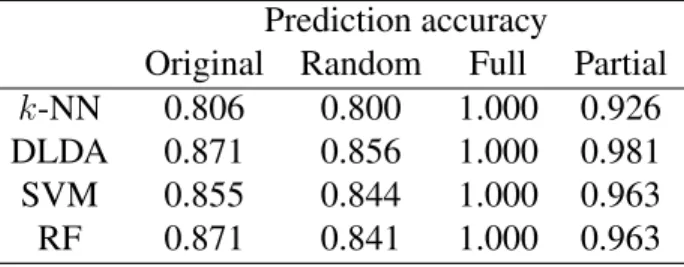
Table 1: Prediction accuracy of four classifiers using LOOCV on the colon cancer data set. The original data set, the data sets after removal of random samples, and the data sets after partial and full removal of outliers are compared.
shown to be amongst the best performing classifiers on microarray data (Dudoit et. al., 2002; Lee et. al., 2005).
We compared the original data set, the data sets after removal of random sam-ples, and the data sets after full and partial removal of outliers. The data sets after random removal of samples were included to demonstrate that simply removing samples does not improve prediction accuracy and were constructed by drawing five sets of eight samples, or the number of outliers, uniformly without replacement from the original data set and removing them. The prediction accuracy was aver-aged over the five resulting data sets. The data set after full removal of outliers was included to demonstrate the overall effect of outliers on prediction accuracy and was constructed by removing the outliers from the original data set. The data set after partial removal of outliers was included to isolate the effect of outliers on the classification of other samples and was constructed by including the outliers in the training data sets, but removing the outliers from the validation data sets.
The results of the comparison are shown in Table 1. The prediction accuracy of the classifiers on the original data set was between 80% and 90%, which is consis-tent with the results of an extensive comparison of classifiers in Lee et. al. (2005). The classifiers performed similarly after randomly removing samples, suggesting that simply removing samples does not affect prediction accuracy. Surprisingly, all four classifiers were able to achieve perfect prediction accuracy after full outlier removal, suggesting that the outliers were the main cause of errors in the clas-sifiers. The outliers seemed to be impossible to classify rather than difficult to classify since the outliers were misclassified by all four classifiers, which are di-verse in their theoretical approach. It is important to note that the outliers were not the only misclassified samples. If only the outliers were misclassified, then the improved prediction accuracy would only show the trivial effect of removing misclassified samples. However, the classifiers also performed better after partial outlier removal, suggesting that the outliers had a negative effect on the training of the classifiers and caused other inlier samples to be misclassified. The difference
in the prediction accuracy between full outlier removal and partial outlier removal indicates how adversely the classifiers were affected by the outliers. The significant performance improvement of the classifiers after outlier removal validates the out-liers identified by our outlier detection method and demonstrates the importance of outlier removal for accurate class prediction.
3.5
Estimation of outlier detection accuracy
Evaluating an outlier detection method on selected data sets demonstrates an ability to identify substantively meaningful outliers, but it does not demonstrate a general ability to identify outliers accurately. It is important to evaluate the performance of an outlier detection method over a large number of data sets. However, estimating the accuracy of an outlier detection method is difficult because there are usually no known outliers in microarray data. Therefore, in order to generate multiple test data sets with different outliers for validation, outliers must be simulated. It is preferable to avoid simulating outliers from a generative model since it is not clear that any generative model is appropriate for microarray data. Rather than directly simulating outliers, we can take advantage of the fact that each class is treated independently for outlier detection. Since an outlier can come from any class that is not observed, we can change the class labels of samples in order to simulate outliers.
We propose a simple method for estimating outlier detection accuracy based on resampling. Consider a data setDcontainingn samples partitioned intok classes Di each containing ni samples, where i = 1, . . . , k. First, one class N = Di containingnN =ni samples must be selected to serve as the set of inlier samples, which we will refer to as the inlier class. The sample sizenN must be large since
the inlier class will form the basis for each test data set. Then the otherk−1classes O =D \ N containing then−nN remaining samples will serve as the set of outlier
samples, which we will refer to as the outlier class. Samples from the outlier class O are outliers in the inlier class N since they come from different classes in the data set. Therefore, we can drawm sets ofh outliersHi from the outlier classO uniformly without replacement and merge them with the inlier classN in order to generatemtest data setsTj = N ∪ Hj, where j = 1, . . . , m. Since the outliers in the test data sets are known, they can be used for validation.
We estimated the outlier detection accuracy on the colon cancer and SRBCT data sets, using the tumor and normal classes in the colon cancer data set and the EWS and RMS classes in the SRBCT data set as the inlier classes. For each inlier class, m = 1000,2000,3000,4000,5000 test data sets containing h = 1,2,3,4,5 outliers respectively were generated and our outlier detection method was applied. Five principal components were selected for each test data set for the sake of sim-plicity. The NB and BL classes in the SRBCT data set were not used as inlier classes
Number of outliers
1 2 3 4 5
Colon cancer Tumor Sensitivity 0.910 0.806 0.741 0.677 0.593 Specificity 1.000 1.000 1.000 1.000 1.000 Normal Sensitivity 1.000 1.000 1.000 1.000 0.996 Specificity 1.000 1.000 1.000 1.000 1.000 SRBCT EWS Sensitivity 1.000 0.999 0.998 0.961 0.914 Specificity 1.000 1.000 1.000 1.000 1.000 RMS Sensitivity 1.000 0.941 0.911 0.842 0.785 Specificity 1.000 0.998 0.997 0.998 0.998 Table 2: Sensitivity and specificity of our outlier detection method using resampling on the colon cancer and SRBCT data sets.
because of their small sample sizes. The outlier detection accuracy was measured by sensitivity, the proportion of true positives to true positives and false negatives, and specificity, the proportion of true negatives to true negatives and false positives, where a positive is an outlier and a negative is a inlier. Since outliers are usually removed, it is important that outliers be identified confidently so that good data is not accidentally thrown away. Therefore, specificity is valued over sensitivity for outlier detection.
The results of the estimation are shown in Table 2. The specificity of our outlier detection method was almost always perfect regardless of the number of outliers and the inlier class used, suggesting that our outlier detection method can be used confidently in general. In fact, our outlier detection method only identified false positives for test data sets where the inlier class used was the RMS class and sev-eral outliers were drawn from the NB class. The NB and RMS classes are located closely in the feature space and it seems that introducing certain samples from the NB class into the RMS class changed the structure of the data significantly. There-fore, the few false positives were likely caused by a problem with our method of simulating outliers rather than a problem with our outlier detection method. The sensitivity of our outlier detection method varied depending on the number of out-liers and the inlier class used. For low numbers of outout-liers, the sensitivity of our outlier detection method was almost always perfect. As the number of outliers in-creased, the sensitivity of our outlier detection method decreased as expected since the outliers were more influential on the structure of the data. Nevertheless, the sen-sitivity of our outlier detection method was still high with as many as five outliers. Since there are usually few outliers in microarray data, our outlier detection method can be expected to perform well in general.
4
Conclusion
In this paper, we proposed a simple, automatic outlier detection method for microar-ray data based on PCA and robust estimation. Existing outlier detection methods for microarray data rely heavily on class information and are not able to identify all types of outliers. Our outlier detection method treats each class independently and can identify outliers with respect to a single class. Additionally, our outlier detection method is fast and can be easily used as a preprocessing step. The im-plementation of our outlier detection method in R had typical runtimes of a few seconds on standard personal computers. Our outlier detection method uses well established methods in the outlier detection literature and is closely related to ro-bust PCA methods from the chemometrics literature such as ROBPCA that also deal with high dimensional data.
We demonstrated the effectiveness of our outlier detection in two ways. First, we showed that our outlier detection method can identify biologically meaningful outliers by validating against known outliers in two benchmark data sets. Then, we showed that our outlier detection method has good general accuracy by simulating a large number of test data sets with known outliers to validate against. Moreover, we showed the importance of outlier detection by demonstrating that outlier removal can improve the prediction accuracy of several classifiers. Finally, we evaluated the performance of ROBPCA on microarray data and found that ROBPCA produced a large number of false positives and fewer true positives than our outlier detection method. Therefore, our outlier detection method appears to be more suitable for microarray data than ROBPCA.
Some theoretical issues with our outlier detection method remain. We proposed to treat each class independently for outlier detection. By ignoring other classes, our outlier detection method seems to obtain robustness to all types of outliers. How-ever, it may actually be beneficial to incorporate more class information into our outlier detection method. Particularly, using class information in dimension reduc-tion may produce better class separareduc-tion and clearer class definireduc-tions. A supervised dimension reduction method like partial least squares (PLS) could be used instead of PCA. It has been argued that supervised dimension reduction methods produce biased data representations (Khan et. al., 2001). However, it has also been shown that PLS outperforms PCA significantly for class prediction (Nguyen and Rocke, 2002). Therefore, using PLS instead of PCA should be explored. Additionally, our outlier detection relies on a normality assumption in order to determine a thresh-old for outliers. Although we found that the normality assumption worked well in practice, it may not hold as well on other, more complex microarray data sets. Therefore, other methods of determining a threshold for outliers based on weaker assumptions should be explored.
Availability
An R script implementing our outlier detection has been made available at the first author’s web page: http://people.fas.harvard.edu/˜shieh/
References
Alon, U., Barkai, N., Notterman, D. A., Gish, K., Ybarra, S., Mack, D., and Levine, A. J. Broad patterns of gene expression revealed by clustering of tumor and nor-mal colon tissues probed by oligonucleotide arrays. (1999). Proceedings of the National Academy of Science USA,96, 6745–50.
Barnett, V., and Lewis, T. (1994). Outliers in statistical data. New York, Wiley. Baty, F., Jaeger D., Preiswerk, F., Schumacher, M. M., and Brutsche, M. H. (2008).
Stability of gene contributions and identification of outliers in multivariate anal-ysis of microarray data. BMC Bioinformatics,9:289.
Bolstad, B. M., Irizarry R. A., Astrand, M, and Speed, T. P. (2003). A comparison of normalization methods for high density oligonucleotide array data based on variance and bias.Bioinformatics,19, 185–193.
Culhane, A. C., Perriere, G., Considine, E. C., Cotter, T. C., and Higgins, D. G. (2002). Between-group analysis of microarray data. Bioinformatics,18, 1600– 1608.
Davies, P. L. (1987). Behaviour of S-estimates of multivariate location parameters and dispersion matrices.The Annals of Statistics,15, 1269–1292.
Dudoit, S., Fridlyand, J., and Speed, T. P. (2002). Comparison of discrimination methods for classification of tumors using gene expression data. Journal of the American Statistical Association,97, 77–87.
Egan, W.J., and Morgan, S.L. (1998). Outlier detection in multivariate analytical chemical data.Analytical Chemistry,70, 2372–2379.
Filzmoser, P., Maronna, R., and Werner, M. (2008). Outlier identification in high dimensions. Computational Statistics & Data Analysis,52, 1694–1711.
Furey, T. S., Cristianini, N., Duffy, N., Bednarski, D. W., Schummer, M., and Haus-sler, D. (2000). Support vector machine classification and validation of cancer tissue samples using microarray expression data. Bioinformatics,16, 906–914. Hardin, J., and Rocke, D. M. (2005). The distribution of robust distances. Journal
of Computational & Graphical Statistics,14, 928–946.
Hastie, T., Tibshirani, R., and Friedman, J.. (2001). The elements of statistical learning. New York, Springer.
Hubert, M., and Engelen, S. (2004). Robust PCA and classification in biosciences.
Bioinformatics,20, 1728–1736.
Hubert, M., Rousseeuw, P. J., and Vanden Branden, K. (2005). ROBPCA: A new approach to robust principal component analysis. Technometrics,47, 65–79. Hubert, M., Rousseeuw, P. J., and Verboven, S. (2002). A fast method for robust
principal components with applications to chemometrics. Chemometrics and Intelligent Laboratory Systems,60, 101–111.
Khan, J., Wei, J., Ringner, M., Saal, L. H., Ladanyi, M., Westermann, F., Berthold, F., Schwab, M., Antonescu, C. R., Peterson, C., and Meltzer, P. S. (2001). Clas-sication and diagnostic prediction of cancers using gene expression profiling and artificial neural networks. Nature Medicine,7, 673–679.
Lee, J. W., Lee, J. B., Park, M., and Song, S. H. (2005). An extensive comparison of recent classification tools applied to microarray data. Computational Statistics & Data Analysis,48, 869–885.
Li, L., Darden, T. A., Weinberg, C. R., Levine, A. J., and Pedersen, L. G. (2001). Gene assessment and sample classification for gene expression data using a ge-netic algorithm/k-nearest neighbor method. Combinatorial Chemistry & High Throughput Screening,4, 727–739.
Li, L., Weinberg, C. R., Darden, T. A., and Pedersen, L. G. (2001). Gene selection for sample classification based on gene expression data: study of sensitivity to choice of parametrs of the GA/KNN method. Bioinformatics,17, 1131–1142.
Moler, E. J., Chow M. L., and Mian, I. S. (2001). Analysis of molecular profile data using generative and discriminative methods. Physiological Genomics, 4, 109–126.
Nguyen, D. V., and Rocke, D. M. (2002). Tumor classification by partial least squares using microarray gene expression data. Bioinformatics,18, 39–50. Rocke, D. M. (1996). Robustness properties of S-estimators of multivariate
loca-tion and shape in high dimension. The Annals of Statistics,24, 1327–1345. Rousseeuw, P. (1985). Multivariate estimation with high breakdown point.
Mathe-matical Statistics and Applications, 283–297.
Rousseeuw, P., and Leroy, A. M. (1986). Robust regression and outlier detection. Wiley, New York.
Ruppert, D. (1992). Computing S estimators for regression and multivariate lo-cation/dispersion. Journal of Computational and Graphical Statistics,1, 253– 270.
Salibian-Barrera, M., and Yohai, V. J. (2006). A fast algorithm for S-regression estimates. Journal of Computational and Graphical Statistics,15, 414–427. Vanden Branden, K., and Hubert, M. (2005). Robust classification in high
dimen-sions based on the SIMCA method. Chemometrics and Intelligent Laboratory Systems,79, 10–21.
Zhu, M., and Ghodsi, A. (2006). Automatic dimensionality selection from the scree plot via the use of profile likelihood. Computational Statistics & Data Analysis,