Faculty of Sciences
Department of Applied Mathematics, Computer Science & Statistics
University of Granada
Department of Computer Science & Artificial Intelligence Programa de Doctorado en Tecnolog´ıas
de la Informaci´on y la Comunicaci´on
Dealing with Imbalanced and Weakly Labelled Data
in Machine Learning using Fuzzy and Rough Set Methods
Dissertation submitted in fulfilment of the requirements for the degree of Doctor of Computer Science
Sarah Vluymans
March 2018
Supervisors: Prof. Dr. Yvan Saeys Dr. Chris Cornelis
Cornelis guarantee, by signing this doctoral thesis, that the work has been done by the doctoral candidate under the direction of the thesis supervisors and, as far as our knowledge reaches, in the performance of the work, the rights of other authors to be cited (when their results or publications have been used) have been respected.
Ghent, March 2018
Doctoral candidate Thesis supervisors
the best people I know. To Sam and Sander Vluymans, wonderful men and beloved brothers.
Zoals de traditie het voorschrijft gaat een eerste woord van dank uit naar mijn promotoren Yvan Saeys en Chris Cornelis. Ik wens hen te bedanken voor het vertrouwen dat ze in me gesteld hebben en de vrijheid die ze me hebben gelaten vanaf het begin van onze samenwer-king.
Als we een beetje verder kijken, komen we terecht bij Lynn D’eer, Nele Verbiest en Sofie De Clercq, die me op weg hebben gezet om dit doctoraat succesvol af te werken. Mushthofa, of course, for his company until the end. Etienne, voor de korte babbels tussendoor.
The assorted members of the Dambi research group: Sofie Van Gassen, Wouter Saelens, Paco Hulpiau, Pieter De Bleser, Liesbet Martens, Arne Soete, Robrecht Cannoodt, Joeri Ruyssinck, Leen De Baets, Isaac Triguero, Joris Roels, Dani Peralta, Helena Todorov, Quentin Rouchon, Robin Vandaele, Jonathan Peck, Robin Browaeys, Annelies Emmaneel and Niels Vandamme. Particular thanks for the tasty biscuits at our Friday meetings. Dr. Triguero deserves special mention for his unwavering belief in my abilities. Dr. Peralta for helping me out whenever needed.
Nu moet ik zeker mijn andere aangename bureaugenoten van de voorbije jaren nog bedanken, Ludger Goeminne, Bart Van Gasse, Karel Vermeulen en Domien Craens. Uiteraard ook mijn overige TWIST-collega’s waarmee ik samenwerkte om onze studenten in het gareel te houden, Dieter Mourisse, Annick Van Daele en Felix Van der Jeugt.
Naturally, everyone else at S9, my lunch mates, fellow tea drinkers and anyone stopping by for a little chat or a laugh.
Ook nog een dikke merci en mil gracias aan iedereen die me de voorbije jaren met de admini-stratieve rompslomp e.d. heeft voortgeholpen: Hilde, Ann, Wouter en Herbert op S9, Marita op het VIB en Bea y Paco en el CITIC.
Moving on to the more research-related acknowledgements. Having collaborated with sev-eral international colleagues over the years, I would like to express my thanks to Neil Mac Parthal´ain and Richard Jensen at the University of Aberystwyth, Amelia Zafra, Sebastian Ventura and Nicolas Garc´ıa-Pedrajas at the University of C´ordoba, D´anel S´anchez Tarrag´o at the Central University of Las Villas and Martine De Cock, Ankur Teredesai and Shanu Sushmita at the University of Washington Tacoma. Thanks to all my wonderful colleagues at the University of Granada as well for their hospitality and kindness, with a specific word of gratitude to my co-authors Alberto Fern´andez, Juli´an Luengo and, never to be forgotten, Paco Herrera. Much´ısimas gracias to all of you!
apologies for that oversight.
Now for the personal part. Mijn goede vrienden, in het bijzonder Lisa en Liese, bedank ik voornamelijk voor het relativerende inzicht dat dit allemaal maar werk is. Mijn familie, voor hun interesse in mijn vorderingen en hun overtuiging dat ik goed bezig ben.
Rebekka en de jongens, mijn beste broers, om dat ook te zijn.
To conclude, I wish to borrow my final words from my master thesis, which ring true today and forevermore: hartelijk dank aan mijn ouders, die me altijd steunen in alles wat ik doe.
Sarah Vluymans March 2018
Dit doctoraat kwam tot stand met steun van het Bijzonder Onderzoeksfonds van de Uni-versiteit Gent. De buitenlandse verblijven aan de UniUni-versiteit van Granada (Spanje) werden gefinancierd door het Fonds voor Wetenschappelijk Onderzoek Vlaanderen. De experimenten in deze thesis werden deels uitgevoerd op de Hercules rekeninfrastructuur van de Universiteit van Granada.
1 Introduction 1
1.1 Imbalanced and weakly labelled data . . . 1
1.1.1 Imbalanced data . . . 2
1.1.2 Semi-supervised data. . . 3
1.1.3 Multi-instance data . . . 4
1.1.4 Multi-label data . . . 5
1.2 Fuzzy rough set theory . . . 5
1.2.1 Fuzzy sets . . . 6
1.2.2 Rough sets . . . 8
1.2.3 Fuzzy rough sets . . . 9
1.3 Fuzzy rough algorithms in machine learning . . . 11
1.3.1 Fuzzy rough feature and instance selection. . . 11
1.3.2 Fuzzy rough prediction methods . . . 12
1.4 Research objectives and overview of the dissertation . . . 13
2 Classification 15 2.1 Introduction. . . 15
2.2 Classification models . . . 17
2.2.1 Nearest neighbour classification . . . 17
2.2.2 Decision or classification trees. . . 17
2.2.3 Linear models. . . 19
2.2.4 Neural network classification . . . 19
2.2.5 Rule models. . . 20
2.2.6 Probabilistic models . . . 22
2.2.7 Ensemble classification . . . 22
2.3 Conducting classification experiments . . . 24
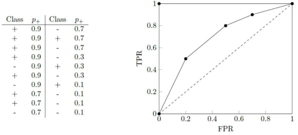
2.3.1 Evaluation measures . . . 24
2.3.2 Validation techniques . . . 27
2.3.3 Statistical analysis . . . 28
3 Understanding OWA based fuzzy rough sets 33 3.1 Ordered weighted average based fuzzy rough sets . . . 33
3.1.1 Fuzzy rough approximations of decision classes . . . 33
3.1.2 Ordered weighted average aggregation . . . 35
3.1.3 OWA based fuzzy rough sets . . . 36
3.2 OWA weighting schemes . . . 37
3.2.2 A data-dependent weighting scheme . . . 42
3.2.3 Preliminary comparison . . . 46
3.3 Lower approximation weighting scheme selection . . . 49
3.3.1 Experimental set-up . . . 49
3.3.2 Motivation . . . 50
3.3.3 Proposed weight selection strategy . . . 51
3.3.4 Detailed discussion . . . 55
3.4 Upper approximation weighting scheme selection . . . 59
3.4.1 Motivation . . . 59
3.4.2 Proposed weighting scheme selection strategy . . . 60
3.5 Guideline validation . . . 62
3.5.1 Guidelines summary . . . 63
3.5.2 Data from Table 3.1 . . . 64
3.5.3 Independent data. . . 65
3.5.4 Other applications . . . 68
3.6 Conclusion . . . 70
4 Learning from imbalanced data 73 4.1 Binary class imbalance . . . 73
4.1.1 The class imbalance problem . . . 74
4.1.2 Dealing with binary class imbalance . . . 74
4.1.3 The IFROWANN method . . . 76
4.2 Multi-class imbalance . . . 78
4.2.1 The one-versus-one decomposition scheme . . . 79
4.2.2 OVO decomposition and the classifier competence issue . . . 80
4.2.3 Dealing with multi-class imbalance . . . 81
4.3 FROVOCO: novel algorithm for multi-class imbalanced problems . . . 82
4.3.1 Binary classifier within OVO: IFROWANN-WIR . . . 83
4.3.2 New OVO aggregation scheme: WV-FROST . . . 84
4.3.3 Overview of the FROVOCO proposal . . . 87
4.4 Experimental study. . . 88
4.4.1 Experimental set-up . . . 88
4.4.2 Evaluation of IFROWANN-WIR . . . 90
4.4.3 Evaluation of IFROWANN-WV-FROST . . . 91
4.4.4 WV-FROST versus other dynamic approaches . . . 94
4.4.5 FROVOCO versus state-of-the-art classifiers . . . 94
4.5 Conclusion . . . 98
5 Fuzzy rough set based classification of semi-supervised data 101 5.1 Semi-supervised classification . . . 101
5.1.1 Self-labelling techniques . . . 102
5.1.2 Other semi-supervised classification techniques . . . 104
5.1.3 Applications . . . 105
5.2 Fuzzy rough set based classifiers and self-labelling. . . 105
5.2.1 OWA based fuzzy rough classifiers on semi-supervised data . . . 106
5.2.2 Interaction with self-labelling schemes . . . 108
5.2.4 Discussion . . . 112
5.3 Conclusion . . . 115
6 Multi-instance learning 119 6.1 Introduction to multi-instance learning . . . 120
6.1.1 Origin . . . 120
6.1.2 Structure of multi-instance data . . . 121
6.1.3 Application areas . . . 121
6.2 Multi-instance classification . . . 122
6.2.1 Multi-instance hypotheses . . . 123
6.2.2 Taxonomy of multi-instance classifiers . . . 124
6.2.3 Imbalanced multi-instance classification . . . 125
6.3 Fuzzy multi-instance classifiers . . . 125
6.3.1 Proposed classifiers . . . 126
6.3.2 Overview of the framework . . . 130
6.3.3 Worked examples . . . 130
6.3.4 Theoretical complexity analysis . . . 132
6.4 Experimental study of our fuzzy multi-instance classifiers . . . 134
6.4.1 Datasets . . . 134
6.4.2 The IFMIC family . . . 135
6.4.3 The BFMIC family. . . 138
6.5 Fuzzy rough classifiers for class imbalanced multi-instance data . . . 140
6.5.1 Proposed classifiers . . . 141
6.5.2 Overview of the framework . . . 144
6.5.3 Theoretical complexity analysis . . . 145
6.6 Experimental study of our fuzzy rough multi-instance classifiers . . . 148
6.6.1 Datasets . . . 148
6.6.2 The IFRMIC family . . . 148
6.6.3 The BFRMIC family . . . 152
6.7 Global experimental comparison . . . 158
6.7.1 Included methods . . . 159 6.7.2 Balanced data . . . 161 6.7.3 Imbalanced data . . . 162 6.7.4 Summary . . . 165 6.8 Conclusion . . . 165 7 Multi-label learning 167 7.1 Introduction to multi-label learning. . . 167
7.1.1 Multi-label data . . . 168
7.1.2 Multi-label classification . . . 168
7.2 Nearest neighbour based multi-label classifiers. . . 169
7.2.1 Basic unweighted approaches . . . 170
7.2.2 Basic weighted approaches. . . 170
7.2.3 MLKNN and related methods. . . 171
7.2.4 Other nearest neighbour based multi-label classifiers . . . 171
7.3 Multi-label classification using a fuzzy rough neighbourhood consensus . . . . 172
7.3.2 Instance quality measure . . . 173
7.3.3 Labelset similarity relation . . . 174
7.3.4 Computational complexity. . . 176
7.4 Experimental study. . . 176
7.4.1 Experimental set-up . . . 177
7.4.2 FRONEC variants . . . 179
7.4.3 Comparison on synthetic datasets . . . 181
7.4.4 Comparison on real-world datasets . . . 188
7.5 Conclusion . . . 191
8 Conclusions and future work 193 8.1 Overview and conclusions of the presented work. . . 193
8.2 Future research directions . . . 196
8.2.1 Dealing with large to massive training sets . . . 196
8.2.2 Data type combinations . . . 198
8.2.3 High dimensionality problem . . . 198
8.2.4 Dataset shift problem . . . 199
8.2.5 Transfer learning . . . 199 Samenvatting 201 Summary 205 Resumen 209 List of publications 213 Bibliography 215
1
Introduction
Generally put, this thesis is on fuzzy rough set based methods for machine learning. We develop classification algorithms based on fuzzy rough set theory for several types of data relevant to real-world applications. Before going into detail on our models, a short introduc-tion to these main components is required. In Secintroduc-tion 1.1, we first present the problem of imbalanced data and several challenging other data types, which can be grouped under the umbrella term of weakly labelled data, for which we develop fuzzy rough set based classifica-tion methods throughout this work. Secclassifica-tion 1.2 provides a brief initiation into fuzzy rough set theory. This mathematical framework for modelling data uncertainty is discussed suffi-ciently detailed, but without going into too much of the mathematical particulars. The latter aspect is reserved for later chapters. We include a general discussion on machine learning with a particular focus on how fuzzy rough set theory has already been used in this domain in Section1.3. Finally, to conclude this introductory chapter, we provide an overview of the thesis in Section1.4.
1.1
Imbalanced and weakly labelled data
Machine learning is a field of study concerned with computer algorithms that enhance their knowledge of or performance in some task through experience [155, 323, 328]. The need for explicit programming is reduced. In this thesis, the concept of experience refers to available information provided in the form of a dataset containing (supposedly) correctly labelled ob-servations. We focus on the task of classification (Chapter 2), which requires a method to construct a prediction model or mechanism based on a collected set of labelled elements (the training set).
In standardsupervisedlearning, the learner is presented with a fully labelled training set, that is, every instance is associated with a known outcome. This outcome can be categorical, in which case the prediction task corresponds toclassification, or continuous, when we consider regression. An instance or observation x can be represented by a feature vector and the ith position in this vector contains the value of x for the ith descriptive feature. A standard supervised training dataset can consequently be represented in a flat table of n rows and d+ 1 columns (with nthe number of instances anddthe number of features). The additional column (commonly the last one) contains the outcome. Table1.1contains an example classi-fication dataset, namely a portion of the widely popularirisdataset created by Robert Fisher
Table 1.1: A portion of theiris dataset.
Sepal length Sepal width Petal length Petal width Class
5.1 3.5 1.4 0.2 Iris Setosa 4.9 3.0 1.4 0.2 Iris Setosa 4.6 3.1 1.5 0.2 Iris Setosa 7.0 3.2 4.7 1.4 Iris Versicolor 6.4 3.2 4.5 1.5 Iris Versicolor 6.9 3.1 4.9 1.5 Iris Versicolor 6.3 3.3 6.0 2.5 Iris Virginica 5.8 2.7 5.1 1.9 Iris Virginica 7.1 3.0 5.9 2.1 Iris Virginica
[153]. The observations are described by four features measuring plant properties. The class label represents the type of iris (setosa, versicolor or virginica). The learning task associated with a supervised training dataset is to derive a prediction model to predict the outcome of newly presented instances of which only the feature values are known.
Several properties of a dataset can render it inherently more challenging to use in a classifi-cation setting. One often encountered issue is an uneven division of observations across the classes, implying that relatively more information is available for some classes than others. The topic ofimbalanced data is briefly introduced in Section1.1.1. Aside from the challenge of a skewed class distribution, the standard dataset format presented in Table1.1can be gen-eralized in several ways. First, we can considersemi-supervised data([72,510], Section1.1.2), which can be placed on the midpoint between supervised (Table1.1) and unsupervised data (Table1.1without the final column). The training set contains both labelled and unlabelled instances and the aim is to combine the information in both to predict the outcome of the unlabelled elements in the training set as well as any newly presented instances. Secondly, we report multi-instance learning ([217], Section 1.1.3). In a multi-instance dataset, each observation is represented by several feature vectors. Together, they form one bag. Only the bag as a whole has an associated outcome, while its constituent instances do not. A third generalization is represented by multi-label learning ([216], Section 1.1.4), where each obser-vation can be associated with more than one class label. Every instance may have a different number of outcomes and relationships between the possible labels can exist. The term multi-label learning is usually reserved for classification tasks, while multi-target learning is used for regression datasets. The three associated dataset formats can be grouped on the common denominator ofweakly labelled data. A taxonomy for weakly labelled data has recently been proposed in [215] based on three axes: (i) the instance-label relationship, (ii) the supervision model in the learning phase and (iii) the supervision model in the prediction stage. The multi-instance and multi-label paradigms relate to the first axis, while the semi-supervised setting relates to the supervision model in the learning stage.
1.1.1 Imbalanced data
Table 1.2 depicts an imbalanced version of the iris dataset. Only two classes are present, setosa and versicolor. The former contains two observations, while the latter consists of six samples. The fact that there are three times as many elements of one class than of the
Table 1.2: An imbalanced version of the irisdataset. Sepal length Sepal width Petal length Petal width Class
5.1 3.5 1.4 0.2 Iris Setosa 4.9 3.0 1.4 0.2 Iris Setosa 7.0 3.2 4.7 1.4 Iris Versicolor 6.4 3.2 4.5 1.5 Iris Versicolor 6.9 3.1 4.9 1.5 Iris Versicolor 6.6 3.0 4.4 1.4 Iris Versicolor 6.7 3.0 5.0 1.7 Iris Versicolor 5.7 2.6 3.5 1.0 Iris Versicolor
other in the training set can inhibit a learning algorithm to construct a strong-performing prediction model, that is, a classifier that would perform well on both classes. Traditional classification methods tend to predict the majority class too often and lead to relatively too many classification errors on the minority class, which is often the class of interest [57,211, 391]. Class imbalance presents itself in many research areas, including medical diagnosis and bioinformatics.
In a two-class imbalanced dataset, the imbalance ratio (IR) is defined as the ratio of the size of the majority class (often called ‘negative’, N) to the size of the minority class (often called ‘positive’, P). In particular, IR = |N||P|. The higher this value, the more imbalance exists between the two classes. When more than two classes are present, this metric can for instance be generalized to IR = max C∈C |C| min C∈C|C| , (1.1)
where C is the set of all classes. Class imbalance, in particular the general setting of an imbalanced dataset with more than two classes, is studied in Chapter 4.
1.1.2 Semi-supervised data
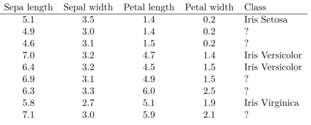
Table 1.3 presents an example semi-supervised dataset. This is the same portion of theiris dataset as in Table 1.1, but not all class labels are known. For some training instances, the outcome is hidden. This type of datasets is commonly encountered in applications where the label assignment is costly or difficult to obtain [510]. As a result, only a (very) small portion of the training instances is labelled, complemented with a (large) number of unlabelled elements. Application areas in which training sets are often only partially labelled include natural language processing, bioinformatics and image recognition. The common characteristic of these domains is that data is often abundantly available or relatively easy to obtain, but challenging or expensive to annotate.
In semi-supervised classification, the goal is to use the information in both the labelled and unlabelled parts to construct a classification model. Insemi-supervised clusteringon the other hand, the labelling information is transformed to a set of constraints to which the clustering method should adhere. Semi-supervised learning is further explored in Chapter 5.
Table 1.3: A portion of theiris dataset in semi-supervised classification. Sepa length Sepal width Petal length Petal width Class
5.1 3.5 1.4 0.2 Iris Setosa 4.9 3.0 1.4 0.2 ? 4.6 3.1 1.5 0.2 ? 7.0 3.2 4.7 1.4 Iris Versicolor 6.4 3.2 4.5 1.5 Iris Versicolor 6.9 3.1 4.9 1.5 ? 6.3 3.3 6.0 2.5 ? 5.8 2.7 5.1 1.9 Iris Virginica 7.1 3.0 5.9 2.1 ? 1.1.3 Multi-instance data
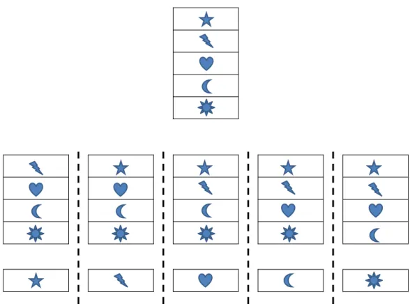
Multi-instance learning was first proposed in [127] to deal with representation ambiguity of training samples. In particular, this study focused on the classification task where several alternative feature vectors represent the same entity. The collection of instances (feature vectors) that make up one observation is called abag. Each bag in a multi-instance dataset can contain a different number of instances, but all instances are described by the same set of features. Two observations contained in the traditional Musk1 dataset, used in the original multi-instance proposal and the bulk of later experimental studies, can be found in Table1.4. Each observation corresponds to a chemical molecule. One and the same molecule can have different conformations or shapes, each corresponding to an instance. This dataset was used in drug activity prediction, where the task is to predict whether a molecule can bind to a given target, making it a so-called good drug molecule. The classification outcome can be ‘positive’ or ‘negative’. A positive class label means that at least one (but not necessarily all) of the conformations of the molecule lead to a target binding. However, as this label is only assigned to the bag as a whole, there is no direct indication which instance has the binding property. The hidden relation between instances and classes renders multi-instance classification a more general and challenging prediction task than traditional single-instance classification.
Table 1.4: Two observations from the multi-instanceMusk1 dataset.
BagID f1 f2 . . . f166 f167 Class MUSK-jf59 52 -110 . . . -60 -29 Positive 49 -98 . . . -13 -12 23 -113 . . . -9 90 47 -110 . . . -5 -8 9 -114 . . . -28 112 NON-MUSK-334 7 -197 . . . 34 55 Negative 25 -198 . . . 20 -8
A recent and thorough review of the multi-instance learning domain can be found in [217]. Application domains can be divided into three general groups. The first group, which includes the drug prediction task described above, consists of fields with different alternative views,
representations or descriptions for the same object. A second branch of multi-instance data sources study compound objects. Each instance corresponds to a particular part of the object. A classic example is the image recognition task, where the image object is divided into several smaller segments. Finally, evolving objects, sampled at different time points, can be modelled as multi-instance data as well. Multi-instance learning forms the focus of Chapter6.
1.1.4 Multi-label data
The multi-label learning domain has been reviewed in e.g. [195,216,484]. As opposed to the traditional classification task associated with the data format in Table1.1, the goal in multi-label classification is to predict the presence of multiple multi-labels at the same time. Every element can belong to more than one category at once and the number of classes can be different for each instance. Example multi-label classification applications are image processing and text categorization. An image or text can naturally belong to multiple classes at the same time, when it depicts several concepts (e.g. a park with playing children) or discusses several topics (e.g. a review of a political play).
As an example, Table 1.5 groups some elements of the Birds dataset [61]. Each instance corresponds to an audio track, labelled with the birds whose song is present in the track. There are 19 possible bird species and several birds can be heard together in some tracks. For example, the third sample contains sounds from three different birds. Chapter7discusses the domain of multi-label learning in more detail.
Table 1.5: Three observations from the multi-labelBirds dataset. f1 f2 . . . f260 Labels
0.054606 0.161667 . . . 8 Swainson Thrush
0.027401 0.015898 . . . 13 Varied Thrush, Hermit Warbler
0.060964 0.187454 . . . 15 Pacific-slope Flycatcher, Varied Thrush, Golden Crowned Kinglet
1.2
Fuzzy rough set theory
In this thesis, we use fuzzy rough set theory in classification algorithms to deal with the challenging data types discussed above. Fuzzy rough sets were proposed in the seminal contribution of [132] as a fusion of two existing mathematical paradigms: fuzzy set theory [473] and rough set theory [342]. In particular, rough sets were generalized to fuzzy rough sets by allowing (or rather, introducing) fuzziness in several strategic places. As such, more flexibility was obtained and several real-world problems could be handled in a more appropriate manner. Both fuzzy and rough sets, discussed in Sections1.2.1 and 1.2.2respectively, aim to capture uncertainty in data. The former does so by modellingvagueness, while the latter focuses on incompleteness orindiscernibility. The combination of the two into fuzzy rough sets implies the ability to model both (complementary) types of data uncertainty. The traditional fuzzy rough set model is recalled in Section1.2.3.
1.2.1 Fuzzy sets
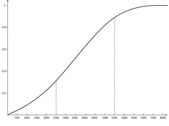
Fuzzy sets were introduced in [473] to model intrinsically vague or subjective notions. In realistic problems, it is not always possible to provide a crisp definition of a concept or a black-and-white division of data into groups. A simple example is the question how to define expensive property in the housing market. Contemplating this problem should immediately demonstrate that it is difficult to find one threshold above which any property should be considered expensive. This threshold may be context-dependent, since one could for example expect different cut-offs to apply for expensive apartments or expensive mansions. The prob-lem is also naturally subjective, because a wealthy person may employ a higher threshold than a less-privileged one. Another issue is the artificial division this threshold-based ap-proach implies. Suppose the threshold ofe400000 has been selected. A property of e401000 would be considered expensive, while one of e399000 would not be so. The difference in these prices would be negligible for most buyers and yet they lead to a different assignation of ‘expensive’ and ‘not expensive’. Finally, one can also oppose the lack of gradation present in the crisp definition of expensive property. Two houses costing half a million and five million euros respectively would both be considered expensive without making a further distinction between them. 50k 100k 150k 200k 250k 300k 350k 400k 450k 500k 550k 600k 650k 700k 750k 800k 1 0.4 0.6 0.2 0.8
Figure 1.1: Example membership curve for the fuzzy set of expensive property.
These issues can be resolved by allowing a graded membership of elements to a set. In traditional set theory, an element either belongs to a set or it does not. Fuzzy sets allow elements to belong to them to a certain degree. The membership function A(·) associated
with a fuzzy set takes on values in the unit interval [0,1]. At the lower end of the spectrum, A(x) = 0 indicates that element x does not belong to A at all. The other extreme A(x) = 1 means that x fully belongs to A. Any value between 0 and 1 corresponds to a partial membership of the element to the set. Figure 1.1presents an example membership function for the fuzzy set of expensive property. As common-sense dictates, this is an increasing function. The left dashed line shows that a house costinge250000 has a membership degree of about 0.3 to this set, meaning that it is not considered all that expensive. On the other hand, a house price ofe550000 (represented by the right dashed line) is considered sufficiently steep and has a membership degree of about 0.9. Fuzzy set theory clearly provides us with a flexible tool to address the issues listed above. Aside from set membership, the same ideas can be incorporated in fuzzy relations and fuzzy logic, discussed in the following paragraphs. In traditional set theory, a relation between elements can be represented as a set of pairs. If the pair (x1, x2) belongs to this set, the two elements are related. This results in a similar crisp delineation between instances that are related to each other and instances that are not. It does not allow one to express the degree to which two instances are related. This issue is dealt with by introducing a fuzzy relation, defined as a mapping from the set of all possible pairs of elements to the unit interval. For a fuzzy relation R, value R(x1, x2) expresses the degree of relatedness ofx1 and x2. The closer this value is to one, the stronger the relation between the two instances.
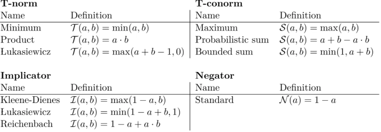
Table 1.6: Example fuzzy logic operators: t-norms, t-conorms, implicators and a negator.
T-norm T-conorm
Name Definition Name Definition
Minimum T(a, b) = min(a, b) Maximum S(a, b) = max(a, b) Product T(a, b) =a·b Probabilistic sum S(a, b) =a+b−a·b Lukasiewicz T(a, b) = max(a+b−1,0) Bounded sum S(a, b) = min(1, a+b)
Implicator Negator
Name Definition Name Definition
Kleene-Dienes I(a, b) = max(1−a, b) Standard N(a) = 1−a Lukasiewicz I(a, b) = min(1−a+b,1)
Reichenbach I(a, b) = 1−a+a·b
Fuzzy logic extends traditional Boolean logic to the fuzzy setting [262]. Fuzzy logic operators have been defined to generalize the principles of conjunction, disjunction, implication etc. A triangular norm (t-norm)T : [0,1]2 →[0,1] is a commutative and associative operator that is increasing in both arguments and upholds the boundary condition (∀a∈[0,1])(T(a,1) =a). It is related to the Boolean conjunction, as is evident when the domain is restricted to{0,1}. A fuzzification of the Boolean disjunction is represented by atriangular conorm (t-conorm) S: [0,1]2 →[0,1], which is also commutative, associative and increasing in its two arguments, but has 0 as neutral element, that is, (∀a∈ [0,1])(S(a,0) =a). A third group of operators consist of so-calledimplicators I : [0,1]2 →[0,1], that are decreasing in their first argument, increasing in the second and satisfy the boundary conditionsI(0,0) =I(0,1) =I(1,1) = 1 andI(1,0) = 0. They form the fuzzy extension of traditional implication, as is evident from the boundary conditions. Finally, the Boolean negation is extended to anegator N : [0,1]→
[0,1], which is a decreasing operator that satisfiesN(1) = 0 andN(0) = 1. A wide variety of choices for operatorsT,S, I and N exist in the literature, examples of which can be found in Table 1.6.
1.2.2 Rough sets
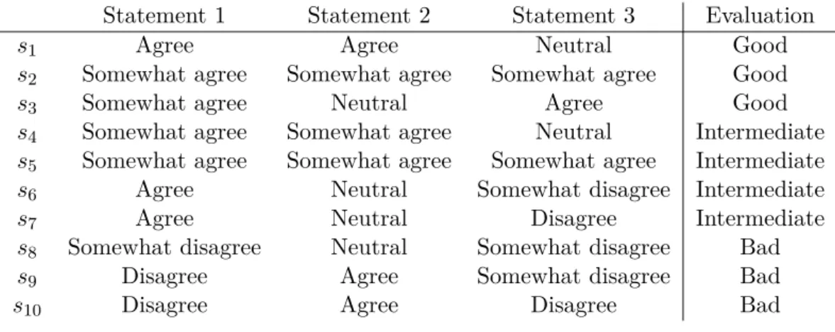
Rough set theory was proposed in [342]. A rough set consists of two sets which together ap-proximate a given incomplete concept. Incompleteness should be understood as the inability of the measured features to discern the concept. Consider the example of course evaluation data provided by university students. At the end of a teaching term, it is common practice to ask students to fill in a questionnaire on courses they have taken. Assume that there are three statements that the student needs to reply to, namely ‘The course met my expecta-tions.’, ‘The pace of teaching was appropriate.’ and ‘The exercises were a fitting addition to the theory classes.’. For each of these, the students can select one of the options ‘Agree’, ‘Somewhat agree’, ‘Neutral’, ‘Somewhat disagree’ and ‘Disagree’ as their response. They are also required to give an overall evaluation of ‘Good’, ‘Intermediate’ or ‘Bad’. A small example dataset based on such an inquiry is depicted in Table 1.7.
The task could be to derive a definition of a good course based on the replies of the students to the three statements. However, based on the data collected in Table 1.7, an unambiguous delineation is not possible. The second and fifth student have each replied ‘Somewhat agree’ to each of the statements, based on which they assign the course a ‘Good’ and ‘Intermediate’ overall evaluation respectively. This shows that the evaluated feature set is incomplete: two elements of different classes coincide in all feature values.
Table 1.7: Example data collected from student evaluations on a particular university course. Each row corresponds to the answers of one student.
Statement 1 Statement 2 Statement 3 Evaluation
s1 Agree Agree Neutral Good
s2 Somewhat agree Somewhat agree Somewhat agree Good
s3 Somewhat agree Neutral Agree Good
s4 Somewhat agree Somewhat agree Neutral Intermediate s5 Somewhat agree Somewhat agree Somewhat agree Intermediate
s6 Agree Neutral Somewhat disagree Intermediate
s7 Agree Neutral Disagree Intermediate
s8 Somewhat disagree Neutral Somewhat disagree Bad
s9 Disagree Agree Somewhat disagree Bad
s10 Disagree Agree Disagree Bad
Rough set theory approximates the class of good courses in two ways. The lower approxi-mation is the set of elements (i) which belong to this class and (ii) for which all elements with exactly the same feature values also belong to the class. Based on Table1.7, the lower approximation of ‘Good’ consists of studentss1 and s3. It can be interpreted as the set of elements thatcertainly belong to this concept, as there is no evidence against their member-ship. It is a conservative approximation. Theupper approximation on the other hand derives a liberal approximation of the ‘Good’ class. This set contains all instances for which there is
at least one data point with exactly the same feature values and the ‘Good’ evaluation. In this case, the upper approximation contains studentss1,s2,s3 and s5.
It should be clear from this simple example that the definitions of the lower and upper approximation entirely rely on the observed feature values. The full feature or attribute set A defines an equivalence relation on the observations, resulting in a partition of the elements into equivalence classes. The equivalence class [x] of elementx is defined as
[x] ={y|(∀a∈ A)(a(x) =a(y))}. (1.2) In this expression, a(x) anda(y) correspond to the values of feature afor elements x and y respectively. It should be clear that the equivalence class ofx consists of all instancesy that have exactly the same feature values as x. Based on this equivalence relation, the lower and upper approximation of a conceptC in dataset T can be defined as
C={x|x∈T,[x]⊆C} and
C ={x|x∈T,[x]∩C6=∅}
respectively. The former consists of elements for which the equivalence class is entirely con-tained inC, while the latter groups elements for which the equivalence class has a non-empty intersection withC. An alternative (but equivalent) formulation of these sets is
x∈C ⇔(∀y∈T)(y∈[x]→y∈C)⇔(∀y∈T)((x, y)∈R→y∈C) (1.3) and
x∈C ⇔(∃y∈T)(y∈[x]∧y∈C)⇔(∃y∈T)((x, y)∈R∧y∈C), (1.4) where Ris the crisp equivalence relation defining the equivalence classes. As briefly noted in Section1.2.1, any traditional relation can be represented as a set of pairs of related elements. Rough set theory forms an ideal tool to approximate indiscernible concepts in datasets of the format represented in Table 1.7. However, an important limitation lies with its use of the equivalence classes (1.2). The case of categorical data, where each feature can take on a finite (and limited) amount of possible values, is handled appropriately by using (1.2). In the presence of continuous numerical data, the interpretability of this definition is reduced. It is unlikely for instances to exactly coincide in a numerical feature, even though their values may be close together. The equivalence classes will consequently often be singletons, such that the core intuition behind the lower and upper approximations is lost. A solution would be to divide the range of numerical features into several intervals by means of discretization [189]. These intervals can be interpreted as categories, but any discretization process will result in information loss, which may therefore not be the ideal fix. A second limitation is that, similar to the vagueness issue discussed in Section 1.2.1, the definitions of C and C assume that C is a traditional crisp set.
1.2.3 Fuzzy rough sets
To deal with the restraints associated with rough sets in general datasets, fuzzy rough set theory has been proposed in [132]. The authors introduced fuzziness into the rough set
operators. In particular, both the approximated concept and similarity between elements are allowed to be fuzzy, the former modelled by a fuzzy set and the latter by a fuzzy relation. One of its crucial components is the fuzzy relationRmeasuring similarity between elements. For two instances x and y,R(x, y)∈[0,1] represents how strongly they are related or, more precisely, how similar we consider them to be. This fuzzy relation replaces its crisp relative appearing in (1.3-1.4). We can fuzzify each component within these expressions to derive the definitions of the fuzzy rough lower and upper approximations. These are fuzzy sets, to which every instance in T has a membership degree between zero and one. The fuzzy rough lower approximation of a (possibly fuzzy) conceptC is defined as
C(x) = min
y∈T[I(R(x, y), C(y))]. (1.5)
Aside from the use of the fuzzy relationR, the universal quantifier in (1.3) has been replaced by a minimum operator, the implication has been generalized to an implicator (see Section1.2.1) and the membership of y to the fuzzy set C is represented by its membership degree. By using the minimum instead of infimum operator, we have assumed that T is finite. This will be the case in both this thesis and real-world applications. In a similar way, the fuzzy rough upper approximation of C is derived as
C(x) = max
y∈T[T(R(x, y), C(y))], (1.6)
where the maximum operator has replaced the existential quantifier and a t-norm is used instead of the crisp conjunction. Expressions (1.5-1.6) correspond to the general implicator/t-norm fuzzy rough set formulation proposed in [358].
As stated above, fuzzy relation R:T2→[0,1] expresses the degree of similarity between two elements inT. Usually, one assumes that this relation is at least reflexive ((∀x∈T)(R(x, x) = 1)) and symmetric ((∀x, y ∈ T)(R(x, y) = R(y, x))). When R has both these properties, it is called a fuzzy tolerance relation. If a fuzzy tolerance relation is also T-transitive with respect to some t-norm T ((∀x, y, z ∈T)(T(R(x, y), R(y, z))≤R(x, z))), it is called a fuzzy T-similarity relation.
A consequence of the use of the minimum and maximum operators in (1.5-1.6) is that the C(x) andC(x) membership degrees are highly sensitive to noise and outliers present in dataset T. Indeed, the addition of one element y to T can have a large effect on these definitions, since it can lead to a new minimum value in (1.5) or a new maximum value in (1.6). This poor noise robustness of traditional fuzzy rough sets has been pointed out in several places in the literature and a variety of noise-tolerant fuzzy rough set models have afterwards been proposed to address this issue [118, 229]. These include β-precision fuzzy rough sets [150], variable precision fuzzy rough sets [324,325], vaguely quantified fuzzy rough sets [106], fuzzy variable precision rough sets [493], soft fuzzy rough sets [224,225], ordered weighted average based fuzzy rough sets [108], variable precision fuzzy rough sets based on fuzzy granules [461] and a data distribution aware fuzzy rough set model [15]. Among them, ordered weighted average based fuzzy rough sets can be considered a preferred alternative, both theoretically and empirically [118]. This model is studied in detail in Chapter3.
1.3
Fuzzy rough algorithms in machine learning
As stated above, we focus on the classification task, in which a prediction model is derived from a set of labelled observations. Nevertheless, the field of machine learning far exceeds the classification domain. In this section, we provide a brief overview of popular settings and, at the same time, indicate how fuzzy rough set theory has been used in these domains in the literature [421].
Two fundamental stages of the knowledge discovery process are data preprocessing and data mining [102]. The recent review [189] divides the former into data preparation and data reduction methods. A data preparation step converts raw data to an appropriate format by, for example, cleaning or transforming the data. Data reduction methods include such popular techniques as feature selection (reduction of the number of descriptive features, [297]), instance selection (reduction of the number of observations, [296]), feature extraction (creation of new features, [295]), instance generation (creation of new instances, [404]) and discretization (transformation of the continuous features to categorical features, [190]). We discuss the use of fuzzy rough set theory for feature and instance selection in Section1.3.1.
Once the data has been shaped into the correct format and possibly improved by a data reduction technique, the aim is to extract the hidden information it contains. Concretely, this can be the construction of a prediction model based on the available information or the discovery of patterns or structures in the observed data. Section1.3.2 provides more detail on this step and the different subdomains where fuzzy rough set theory has been used. General (but thorough) introductions to machine learning can be found in e.g. handbooks [155, 328]. For more details on the use of fuzzy rough set theory in this area and more complete references, we refer the interested reader to our review paper [421].
1.3.1 Fuzzy rough feature and instance selection
Feature selection has been and remains a favoured application domain of fuzzy rough set theory. Advances continue to be made. The shared aim of fuzzy rough feature selection methods is to reduce the full feature set to a strong subset with the same (or possibly better) discerning capacity. In a classification context, it is not necessary to be able to discern between each pair of instances, only if they belong to different classes. Indeed, the fundamental goal of classification is to extract an effective separation between classes and not between individual instances. The unifying study of [107] uses a general monotone fuzzy rough set based measure M, for which different concrete alternatives are discussed, to assess the ability of a feature subsetBto discern between elements of different classes relative to the same ability of the full feature setA (with M(A) = 1). Different approaches can be taken to optimize Min order to construct a feature subset that approaches the classification capacity ofAto a satisfactory degree.
A first group of fuzzy rough feature selection methods are those based on a discernibility matrix. In rough set theory, the discernibility matrix is defined as an n×n matrix, n being the number of observations in the dataset, where each entry corresponds to a pair of instances and contains a list of features by which the two elements can be discerned (set to ∅ for same-class instances). As explained in Section 1.2.2, a discerning feature is one for
which the two instances take on a different value. In order to discern between the same amount of instances as the full feature set does, it suffices that the reduced set contains one feature of each entry in the matrix. This idea forms the foundation of rough feature selection methods based on a discernibility matrix. In fuzzy rough set theory, this concept is generalized to a fuzzy discernibility matrix. As Section 1.2.3described, the discernibility of instances is no longer a black-and-white matter, as they can be (dis)similar to a certain degree. As for the rough set definition of the discernibility matrix, matrix entries are a set of attributes. However, in the fuzzy setting, they are determined for pairs of sufficiently dissimilar and opposite-class instances. The selected attributes are those for which the values of the two instances are distinct enough. After the construction of the discernibility matrix, the discernibility function can be derived from it. When this function is transformed to the correct form, it represents all feature subsets satisfying the discerning capacity requirement (as well as an additional minimality condition). Example fuzzy rough set methods include [85, 87,88,89,90, 214,409,494]. Unfortunately, the transformation step, which often boils down to the conversion of a function in conjunctive normal form to disjunctive normal form, can be very time consuming. Additionally, it may be sufficient to derive a single good feature subset instead of multiple ones.
To address this shortcoming, faster algorithms using search heuristics have been proposed as well. Several proposals construct the requested feature subset by optimizing the quality measure in an iterative approach. Typically, a forward search is applied that starts from an empty feature subset and adds features until a sufficiently high value of the chosen measure M is reached. In each iteration, the feature with the highest quality (according to some specific criteria) is added to the current set. Another option is to iteratively remove certain features fromAuntil a decrease inMis observed. In fact, almost any search heuristic could be applied. Examples of methods incorporating this idea can be found in e.g. [43,126,213, 226,227,244,245,247,349,352,425,487].
Fuzzy rough instance selection methods have been proposed in [241,360,414,415,417]. They rely on the fuzzy rough approximation operators to decide which instances should be kept in the dataset and which should be removed, e.g. because they are noisy. The combination of feature and instance selection has been considered as well [122,125,312].
1.3.2 Fuzzy rough prediction methods
A general distinction can be made between supervised and unsupervised learning. The former deals with datasets in which all observations are associated with an outcome. The aim is to use these elements to predict the unknown outcome of new observations. Supervised approaches include neural networks [47], support vector machines [377], Bayesian learning [25], instance-based learning [8], rule induction [170] and decision tree learning [366]. In unsupervised learning on the other hand, the observations are not associated with an outcome and the goal is simply to discover structures or relations in the data. We can list clustering [7] and association rule induction [2] as general unsupervised learning techniques. A third setting is semi-supervised learning, which has been introduced in Section1.1.2. We provide a short overview in the following paragraphs.
Supervised learning Arguably the most natural application of fuzzy rough set theory in classification lies with instance-based learning or nearest neighbour approaches. A nearest neighbour classifier is a lazy learner, meaning that it does not construct an explicit prediction model, but rather stores the full dataset to use in the classification of a new instance [110]. It does so by locating itsknearest neighbours among the stored prototypes and aggregating their outcomes to a prediction, commonly by means of a majority vote. As the k nearest neighbours of an instance correspond to itskmost similar elements, it is clear that a nearest neighbour method at its core relies on a similarity or distance relation, as does fuzzy rough set theory (Section 1.2.3). Fuzzy rough nearest neighbour classifiers have been proposed in e.g. [46, 242, 353, 361, 370, 416]. These methods introduce the use of the fuzzy rough approximation operators within the nearest neighbour classification idea.
Fuzzy rough set theory has been applied in decision tree learning as well, mainly in the splitting phases of the tree generation process. A decision tree is constructed by starting from a root node and iteratively splitting nodes into several child nodes with the aim of increasing the purity of leaf nodes. Each split is based on the values of the observations for a particular feature. In traditional decision trees, the selection of a splitting feature relies on measures like the information gain or impurity reduction [155], but this is where fuzzy rough alternatives have been integrated as well [14,44,137,246,479].
Fuzzy rough rule induction methods constructing fuzzy decision rules have been proposed in e.g. [200,221,243,301] and we encounter uses in support vector machines (e.g. [84,86]) and neural networks (e.g. [180,181,184,371,372]) as well. Aside from classification, fuzzy rough regression algorithms, where the outcome is a real number rather than a class label, have been proposed as well (e.g. [16,242]).
Unsupervised learning In the study of [280], a fuzzy rough evaluation measure for the similarity between clusters was introduced in the fuzzyc-means clustering method [42]. This clustering technique constructscsoft clusters from the original data, to which every instance has a certain membership degree. A more advanced clustering method is the self-organizing map procedure [209], to which a fuzzy rough approach was taken in [182,183].
Semi-supervised learning Comparatively little work has been done in the area of fuzzy rough sets for semi-supervised learning. A fuzzy rough set based self-labelling approach, which extends the labelled part of the data by assigning classes to some unlabelled elements, has been proposed in [311]. We can also refer to Chapter 5 for the application and study of fuzzy rough set theory in semi-supervised classification.
1.4
Research objectives and overview of the dissertation
In this thesis, we focus on several challenging classification tasks and wish to develop new machine learning techniques based on fuzzy rough set theory to solve them. We structure our work as follows:
• Chapter2: we first review the classification domain. We discuss more theoretical aspects like the bias-variance trade-off as well as prominent examples of classification algorithms.
This chapter also describes the methodology to set up experimental studies comparing groups of classifiers.
• Chapter 3: this chapter considers the ordered weighted average based fuzzy rough sets proposed in [108]. This is a noise-tolerant extension of the traditional fuzzy rough set model. As this is the model used in our proposed methods in later chapters, it warrants a deeper study. In particular, the choice of weighting scheme is an important question, as it is the key component in determining the fuzzy rough lower and upper approximations of this model. We study the suitability of different weight settings within the class approximations on a variety of datasets and aim to evaluate if, based on simple dataset characteristics, a weighting scheme selection strategy can be proposed to facilitate the use of ordered weighted average based fuzzy rough sets.
• Chapter 4: the first machine learning task we focus on is that of class imbalance, that is, an uneven distribution of observations among the classes (see Section 1.1.1). Some classes appear in abundance, while others are rarely encountered. This poses a challenge to traditional learners and can severely hinder the construction of a strong prediction model. We wish to develop a fuzzy rough set based classifier to handle multi-class imbalanced data and compare it against the current state-of-the-art in this domain. • Chapter 5: in this chapter, we turn our attention to semi-supervised classification (see
Section 1.1.2) and want to evaluate the strength of classifiers based on the ordered weighted average based fuzzy rough set model in this setting. Using the weighting scheme selection strategy proposed in Chapter 3, we test whether these methods can extract sufficient information from the labelled part of the data without requiring any explicit labelling step of the unlabelled observations or whether the latter is necessary to guarantee a strong performance, in particular in relation to existing proposals. • Chapter6: this chapter discusses multi-instance classification, briefly introduced in
Sec-tion 1.1.3above. We wish to develop two groups of methods: fuzzy multi-instance clas-sifiers and fuzzy rough multi-instance clasclas-sifiers. The latter will be specifically focused on class imbalanced multi-instance data. Both groups will be set up as multi-instance classifier frameworks, in which several internal parameters can be modified. We will conduct an extensive experimental study to (i) advise the user on suitable settings and (ii) compare our work to the existing methods for (imbalanced) multi-instance classifi-cation.
• Chapter 7: the last classification challenge addressed with our fuzzy rough methods is the multi-label prediction task (see Section 1.1.4), in which several labels are predicted at once. We aim to develop a nearest neighbour based method that relies on fuzzy rough set theory to derive a consensus prediction from the class labelsets of the neighbours of a target instance. The neighbourhood information needs to be summarized in an adequate way, for which we deem the fuzzy rough set model an ideal tool. As before, we will thoroughly compare our proposal to existing nearest neighbour based multi-label classifiers.
• Chapter 8: to conclude this dissertation, the final chapter summarizes our proposals and findings and outlines future research directions.
2
Classification
In this chapter, we review the traditional classification domain, the supervised learning task on which this thesis focuses. Before addressing several challenging classification problems in the next chapters, we first review the core aspects of this popular research area, as would be done in any machine learning course or handbook. Section2.1 provides a brief and general introduction, explaining often referenced aspects as the bias-variance trade-off and the curse of dimensionality. In Section2.2, we review several groups of classification algorithms, repre-sentatives of which are included in the experimental studies conducted throughout this work. The specifics on how to properly set up classification experiments are laid out in Section2.3.
2.1
Introduction
In traditional classification tasks with input space X, an element x ∈X can be represented as a feature vector of length |A|, with A the set of descriptive features. The ith position in this vector corresponds to the value of instance x for the ith attribute. This allows for an easy organization of classification data into the flat table format represented in Table 1.1. Each row corresponds to one observationx ∈X. The last column is commonly reserved for the class label, while the first|A|columns contain the input feature values.
The classification task is to construct a prediction model based on the information contained in a training or learning set of labelled samples. More concretely, if X is the input space andC the set of possible classes, the aim is to learn a mappingf :X → C based on training set T = {(x, Cx)|x ∈ X, Cx ∈ C}. Several approaches to the derivation of f have been
explored in the literature and will be discussed in Section 2.2. Each of them makes internal assumptions on how the information in the training set should be modelled, with the shared aim to find an appropriate approximation of the decision boundary between classes. Apart from extracting sufficient information from the training set, the model should also be able to generalize well to unseen test data and make accurate predictions. A highly complex model can fit the training data perfectly, but, by modelling all peculiarities in this set, can lead to classification errors on new data. This phenomenon is known as overfitting, where the model almost literally learns the training data by heart. On the other hand of the spectrum, underfitting the data leads to a simple (and probably highly interpretable) model, that will, unfortunately, also fail on new data because insufficient information has been learned from the provided labelled samples. An example of these two situations is depicted in Figure2.1, which
(a) Underfitting (b) Overfitting (c) A better boundary Figure 2.1: Illustration of a two-class datasets (circles and plus signs) with three possible
derived decision boundaries.
represents a two-class two-dimensional dataset. The horizontal and vertical axis correspond to the first feature a1 and second feature a2 respectively. In Figure 2.1a, a simple decision boundary is derived, only based on the first featurea1. All elements with an a1 value lower than the selected threshold (left of the vertical line) would be classified as a plus sign, while those with ana1 value exceeding the threshold will be assigned to the circle class. This is a very simple and easy-to-understand decision rule, but can easily lead to misclassifications on both classes. Figure2.1brepresents a situation where the data has been overfitted. A highly complex boundary has been constructed to perfectly separate the elements of the training set. The third option represented by Figure 2.1c likely forms the best compromise between model interpretability, generalization capacity and training information extraction. A linear decision boundary based on both features (sloped line) has been derived. It does not form a perfect partition of the classes in the training set, but probably results in better predictions on new data.
The issue discussed above is related to balancing accuracy and interpretability as well as the bias-variance trade-off [164]. A highly complex model with a large number of parameters to learn will depend more on its training data and can, consequently, be very different when constructed from a slightly modified training set. This model has a high variance and can exhibit a highly different classification behaviour after small changes in its training set. A very simple model will not suffer from this variance issue, but introduces abias to a certain (simple) structure instead. It can be shown that the expected prediction error of the learned model can be decomposed in an expression containing error terms representing the bias and variance. Ideally, both components should therefore be minimized. Unfortunately, lowering the bias of a model usually increases its variance and vice versa. A learning algorithm should balance these two aspects in order to have a strong prediction performance.
Another issue associated with learning from data is the so-calledcurse of dimensionality. The term was introduced in [36] and refers to the fact that the volume of the Euclidean space increases exponentially when more dimensions are added [258]. High-dimensional spaces are inherently sparse (also called empty space phenomenon). This (negatively) affects the suitability of certain classification approaches in high-dimensional data as well as the intuition behind and interpretability of the derived prediction models. For example, any notion of locality is lost, rendering nearest neighbour based methods inappropriate [41]. This is of particular relevance to the work presented in this dissertation, because fuzzy rough set based
classification algorithms are closely related to nearest neighbour approaches, as they also strongly depend on a distance or similarity relation between observations.
2.2
Classification models
A wide spectrum of classification algorithms have been developed in the literature. In this section, we discuss some popular and widely-used approaches and categorize them according to their prediction rationale. Representatives of these groups will be used in the exper-imental studies conducted in later chapters. We consider nearest neighbour classification (Section 2.2.1), decision trees (Section 2.2.2), linear models (Section 2.2.3), neural networks (Section 2.2.4), rule based models (Section 2.2.5), probabilistic models (Section 2.2.6) and ensemble classifiers (Section2.2.7).
2.2.1 Nearest neighbour classification
Arguably one of the most intuitive classification algorithms is theknearest neighbour method (kNN, [110]), withk≥1 an integer number. It is alazy learner, which means that it does not build an explicit classification model or mapping from the input space to the set of possible classes. Instead, all training elements are stored in memory. These elements are also referred to as prototypes. To classify a new elementx, the k elements nearest to it among the stored prototypes are determined. The class that appears most often among these neighbouring elements is predicted for x. When several classes tie for the most appearances, one among them is usually selected at random.
The notion of nearest is enforced by an appropriate distance or similarity measure. The nearest neighbours of x are the kelements with the smallest distance to or largest similarity with x. The traditional Euclidean distance remains a popular distance measure, although alternatives like the HVDM distance [444] are used as well. Another option is to learn an appropriate distance measure (often in the form of a Mahalanobis distance [314]) from the data by means of a metric learning procedure [34,441]. As the kNN classifier entirely relies on distance calculations, it can greatly benefit from the optimization of this measure to fit the data at hand.
In the procedure described above, each selected neighbour has an equal vote in the class decision ofx. An often used alternative is to weigh the contribution of each neighbour based on its distance to the target [133]. To this end, neighbour weights inversely proportional to this distance are imposed. As a result, more distant neighbours influence the class prediction ofx less than near ones.
2.2.2 Decision or classification trees
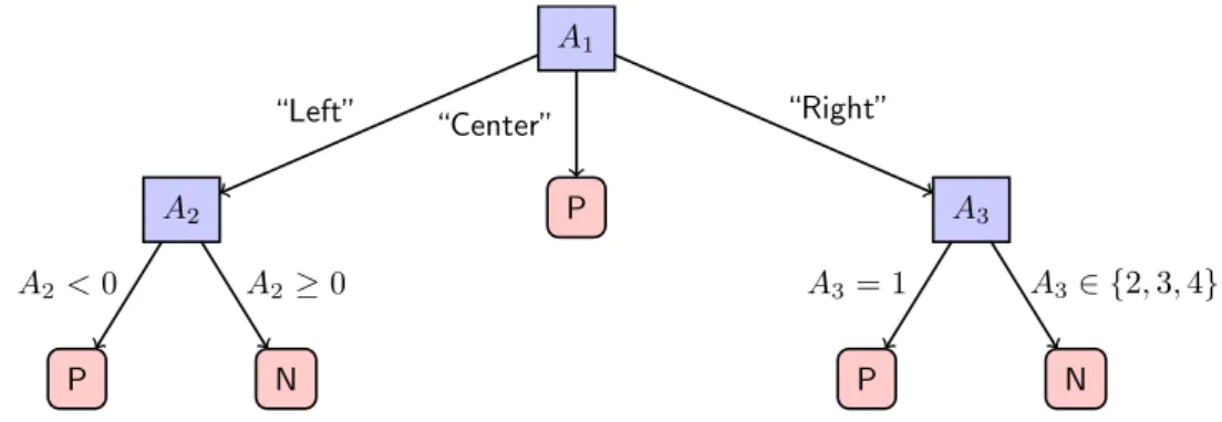
Another popular classification approach is to construct a decision tree based on the training data [366]. A tree is a connected, acyclic graph. Every internal node corresponds to a test based on one of the input features. The leaf nodes, which form end points on paths starting from the root, represent class assignments. To classify a new element, it is passed through the tree, starting at the root node and following the correct path towards a leaf. The class linked to the leaf is assigned to the test element. An example decision tree is depicted in
A1 A2 P A2<0 N A2≥0 “Left” P “Center” A3 P A3 = 1 N A3∈ {2,3,4} “Right”
Figure 2.2: Example of a classification tree prediction whether an instance belongs to the positive (P) or negative (N) class.
Figure 2.2. The first test is made based on the categorical attributeA1. Depending on the feature value, the left, middle or right path is chosen. The left path leads to a second split based on the numeric featureA2. Any value lower than zero leads to an assignment to class P, while elements with positive A2 values are classified as N. On the right hand side, the second split is based on featureA3.
The construction of a decision tree follows a top down procedure. At the outset, the tree consists of the root only and all training instances are grouped together in this node. Based on animpurity measure (assessing the current class distribution) the best feature and corre-sponding split are selected. This split is performed and nodes are created for each possible outcome of the test. The training set is split into subsets corresponding to the division of elements obtained after the test. When a node contains elements of only one class (a pure node), it is retained as a leaf node and labelled with this class. If elements of more than one class are still present, the procedure is repeated and further splits are created starting from this node.
In order to create small trees, the impurity measure guides the split selection process towards feature splits that reduce the class heterogeneity of elements associated with a node. These measures are based on the class distribution in these nodes. When the classes are uniformly distributed within a node, the impurity is maximal. In the presence of only one class, a minimal impurity is found. The CART decision tree algorithm of [60] uses the Gini index as impurity measure, while the ID3 [354] and C4.5 [356] algorithms rely on Shannon’s entropy [379].
If a tree is constructed up to the point when all leaves are pure, there is an increased risk of overfitting the training data and obtaining an overly complex model. A solution to this problem is to apply a pruning procedure [355]. We can discern between pre-pruning and post-pruning. Pre-pruning prematurely halts the tree growing process when a node is considered pure enough or represents too few training instances. Post-pruning allows the full construction of the tree until pure leaf nodes are obtained. Afterwards, branches are removed from the tree to minimize the classification error on a validation set.
2.2.3 Linear models
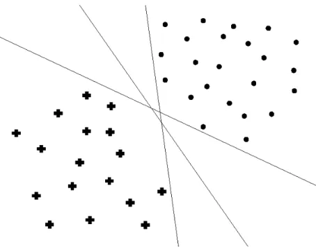
Linear models construct a hyperplane to represent a linear separation between classes. These methods have initially been designed for two-class classification problems. In ad-dimensional space, a hyperplane is a subspace of dimensiond−1. In the two-dimensional plane, a hyper-plane is a straight line. In the three-dimensional space, a hyperhyper-plane is a regular hyper-plane. When two-class data is linearly separable, there exist multiple hyperplanes such that all elements of one class are located on one side and all elements of the second class can be found on the other. However, not all separating hyperplanes are equally suitable, as represented in Figure 2.3. The three straight lines each form a perfect separation between the two classes, but the middle one should be favoured. The proximity of the other two to the training elements is more likely to induce classification errors on test data. The support vector machine (SVM) classifier [54,109,112] implements this idea by maximizing the margin defined by the separating hyperplane. The margin can be interpreted as the (symmetric) empty space around the hyperplane before a training element is encountered. In Figure 2.3, it is clear that the middle hyperplane induces the widest margin between the two classes and is therefore the best option. The search for this hyperplane is formulated as a constrained quadratic optimization problem that can be solved using Lagrange multipliers [40]. To deal with data that is not linearly separable, the soft-margin SVM [109] introduces slack variables that allow elements to be located on the incorrect side of the hyperplane. These slack variables are added to the optimization objective weighted with a penalty termC (the complexity parameter). Another (or additional) way to address the non-linearity of data is to apply an implicit mapping to a different (higher-dimensional) feature space. It can be shown that the SVM formulation and optimization contains only vector dot products, a situation in which thekernel trick can be applied to perform calculations in the induced feature space [9,54]. Example kernel functions are listed in [67]. SVM algorithms are popular and widely used in the machine learning community.
2.2.4 Neural network classification
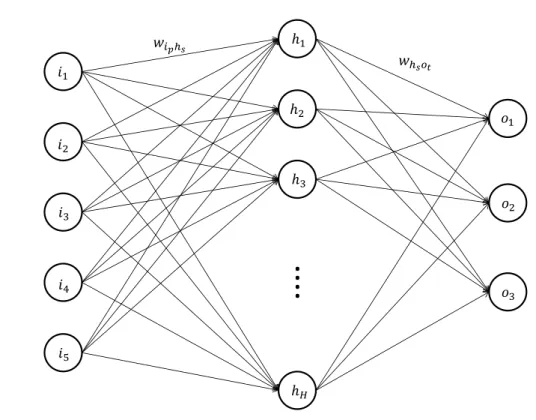
Another linear classification model (but handled in a separate section because of the family of neural network classifiers [47] it inspired) is the perceptron algorithm [337,367]. The normal vector w of the separating hyperplane is randomly initialized. Afterwards, each training element is processed and the values inw are updated to ensure the correct classification of the element. This process is repeated until convergence, that is, until no more changes are made tow. Despite the initial enthusiasm of the research community towards this proposal, [327] pointed out some important limitations of the simple perceptron. These issues were addressed by the later development of the multi-layer perceptron and the back-propagation algorithm [368]. A perceptron can be modelled as a neural network with an input and output layer, while a multi-layer perceptron contains one or more hidden layers. It is a feedforward neural network, where the inclusion of the hidden layers and use of non-linear activation functions allows the modelling of non-linearity in data. An example network is presented in Figure 2.4. Each connection between nodes is associated with a weight, determined at training time by means of the back-propagation procedure. With respect to classification, a neural network classifier for instances in a d-dimensional space often contains d input nodes (one for each feature) andm output nodes, where m is the number of possible classes. The trained network computes one value per output node. The presented instance is assigned to
Figure 2.3: Three separating hyperplanes between two classes.
the class corresponding to the node with the highest value. Research in neural networks has been inspired by the biological neural processes and simulates how neurons work together in the human brain.
The universal approximation theorem implies that a multi-layer perceptron with one hidden layer, final number of nodes and non-linear activation functions can closely approximate any commonly used function [169, 222]. However, the number of hidden nodes required for this task may be large, resulting in an enormous amount of weight parameters to be trained. In recent years, deep learning and deep neural networks have emerged as popular and widely discussed research topics [38,276,376]. Deep neural networks contain several hidden layers. As the number of nodes required per layer can be kept modest, this can result in an exponential reduction in the number of connection weights that need to be trained [38,286]. As a consequence, complex functions can be modelled more efficiently, addressing the issue related with multi-layer-perceptrons mentioned above. Deep neural networks automatically extract features from the data in the form of feature hierarchies. This automation relieves the scientist of the laborious task of determining adequate features, but does imply a lack of interpretability of the final classification model.
2.2.5 Rule models
A rule based classifier derives a set of rules from the dataset and uses these as its prediction model [170]. A rule can be written in the form ‘IF P1 and P2 AND . . . AND Pt THEN C’.
In this expression, Pi (i = 1, . . . , t) are rule premises based on the input features and C is