Computer vision-based limestone rock-type classification using probabilistic neural network

Research paper

Computer vision-based limestone rock-type classi

fi

cation using

probabilistic neural network

Ashok Kumar Patel

, Snehamoy Chatterjee

b_{Department of Geological and Mining Engineering and Sciences, Michigan Technological University, MI 49931, USA}

a r t i c l e i n f o

Article history: Received 1 August 2014 Received in revised form 25 October 2014 Accepted 31 October 2014 Available online 15 November 2014 Keywords:

Supervised classification Probabilistic neural network Histogram based features Smoothing parameter Limestone

a b s t r a c t

Proper quality planning of limestone raw materials is an essential job of maintaining desired feed in cement plant. Rock-type identification is an integrated part of quality planning for limestone mine. In this paper, a computer vision-based rock-type classification algorithm is proposed for fast and reliable identification without human intervention. A laboratory scale vision-based model was developed using probabilistic neural network (PNN) where color histogram features are used as input. The color image histogram-based features that include weighted mean, skewness and kurtosis features are extracted for all three color space red, green, and blue. A total nine features are used as input for the PNN classification model. The smoothing parameter for PNN model is selected judicially to develop an optimal or close to the optimum classification model. The developed PPN is validated using the test data set and results reveal that the proposed vision-based model can perform satisfactorily for classifying limestone rock-types. Overall the error of mis-classification is below 6%. When compared with other three classifi ca-tion algorithms, it is observed that the proposed method performs substantially better than all three classification algorithms.

2014, China University of Geosciences (Beijing) and Peking University. Production and hosting by Elsevier B.V. This is an open access article under the CC BY-NC-ND license (http://creativecommons.org/ licenses/by-nc-nd/3.0/).

1. Introduction

The cement industry provides the main building material for infrastructure and limestone is the main raw material for the cement industry (Ingram and Daugherty, 1991). To meet the increasing cement demands, cement kilns must have consistent and reliable raw material feed. The consequences of poorly pre-pared raw meal are two folds. First, high lime causes meal to be burned hotter and refractory life drops. Second, high alkaline may cause cyclone blockage and restrict the use of the cement produced. Therefore, before feeding the raw material limestone to the cement plant, a proper quality planning is necessary to control the lime and the alkaline proportion in the limestone to the smooth working of the cement plant (Lea, 1971).

Cement industries are taking different measures to maintain the raw material feed quality. Even though all possible measures are

taken to control the quality of feed, thefinal quality of limestone may not respect with the requirements of cement plant (Mayfield, 1988). To deal with this situation, a suitable quality monitoring should be done at mine before sending the limestone at the stockyard for blending process to maintain feed quality for cement plant.

Monitoring the quality of limestone at mine is always a difficult task due to non-availability of fast, reliable and inexpensive on-line sensors. Generally, the limestone quality is determined by manu-ally collecting samples from mine and analyzing chemicmanu-ally in a laboratory and that is tedious and time-consuming operations. However, the quality parameters of the limestone depend largely upon the constituent rock-type; therefore, information about the rock-type provides valuable information for quality monitoring purpose (Tessier et al., 2007).

Although, rock-type information about limestone is valuable for quality monitoring; however, the information about the rock-type at mine can be gathered by visual observation in naked eye by experience geologist or mining engineers. The accuracy of the identification of rock-types varies from person to person and it requires human intervention. Nonetheless, identification of

*Corresponding author.

E-mail address:[email protected](S. Chatterjee).

Peer-review under responsibility of China University of Geosciences (Beijing).

H O S T E D BY Contents lists available atScienceDirect

China University of Geosciences (Beijing)

Geoscience Frontiers

j o u r n a l h o m e p a g e :w w w . e l s e v i e r. c o m / l o c a t e / g s f

http://dx.doi.org/10.1016/j.gsf.2014.10.005

1674-9871/2014, China University of Geosciences (Beijing) and Peking University. Production and hosting by Elsevier B.V. This is an open access article under the CC BY-NC-ND license (http://creativecommons.org/licenses/by-nc-nd/3.0/).

accurate rock-type is a challenging task because of heterogeneity of rock properties. However, with the advancement of the computer vision, rock-type information can be gathered by capturing the rock image. It is frequently experienced that the rock images are non-homogeneous in their shape, texture, and color; and computer vision techniques can analyze complex rock images for rock-type classification purpose.

Although the study of computer vision-based rock-type classi-fication is limited; however, some distinguished results have been reported by researchers (Murtagh and Starck, 2008; Mukherjee et al., 2009; Chatterjee et al., 2010). Computer vision-based sys-tem is introduced in mining industry in the early 90’s byOestriech et al. (1995)when the U.S. Bureau of Mines has developed a sensor system that uses color to instantaneously measure mineral con-centrations in flotation froths and other process streams. Later, lithological composition sensor and ore grindability soft-sensor are developed byCasali et al. (2000)using image analysis.Lepisto et al. (2005) investigated bedrock properties by analyzing the images collected from the bedrock. Different rock layers can be recognized from the borehole images based on the color and texture properties of rock (Lepisto et al., 2005).Tessier et al. (2007)developed an on-line estimation of run-of-mine ore composition on conveyor belts. An application for aggregate mixture grading using image classifi -cation is designed byMurtagh and Starck (2008).Mukherjee et al. (2009) designed an image segmentation system specifically tar-geted for oil sand ore size estimation. Chatterjee et al. (2010)

developed a quality monitoring system of limestone ore grades. Ore grade estimation by feature selection and voting is proposed by

Perez et al. (2011).Khorram et al. (2012) developed a limestone chemical components estimation using pattern recognition.

In vision based technology, data are presented as images. Various information (color, texture and morphological) could be extracted from images. Different researchers have demonstrated the importance of different image features.Khorram et al. (2012)

have used color components, namely r, g, b, H, S, I, and gray for color feature extraction.Perez et al. (2011) have used color and texture feature of a sub image for ore grade estimation. Morpho-logical, color and textural features were used byChatterjee et al. (2010)for quality monitoring system of limestone ore.Mukherjee et al. (2009) used color and morphological features for image segmentation for oil sand ore size estimation.Murtagh and Starck (2008)used texture feature, 2nd, 3rd and 4th order moments of multi-resolution transform coef_ficients as features. Tessier et al. (2007)used color features using multi-way principal component analysis (MPCA) and textural feature using two-dimensional discrete wavelet transform analysis (WTA).Singh and Rao (2006)

studied ferruginous manganese ores with histogram analysis in the RGB color space, combined with textural features based on the gray level co-occurrence matrix and edge detection.Lepisto et al. (2005) used Gabor filtering in Red-Green-Blue (RGB) and Hue-Saturation-Intensity (HIS) color space with different scales to incorporate color in texture features.

Since, it is not known beforehand that which image features have considerable impacts on the rock-type classification; therefore, these algorithms involve extraction of the significant number of features. Thus, the computational time associated with these algo-rithms is significantly larger due to more numbers of parameters associated with the classification model. Nevertheless, the extra image features may sometime lead to a poor model performance (Steppe et al., 1996; Micheletti et al., 2014). Also, the number of training samples necessary for model development grows expo-nentially as the number of features grows (Duda and Hart, 1973).

Therefore, reduction of the dimensionality or selection of some features is necessary for valid models (Narendra and Fukunaga, 1977; Chatterjee and Bhattacherjee, 2011). The limitations of

these approaches are multifolds; especially, feature extraction time is still significantly very large and sometimes requires huge computational time. This limitation can be overcome by generating limited number significant features; therefore, the computation time for feature extraction and training of the classification model can be significantly reduced.

In this paper, a computer vision-based model was developed for limestone rock-type classification. A new set of significant image features was extracted from limestone rock images and probabilistic neural network (PNN) was applied for classification purpose. The parameter of PNN model is selected by cross-validation study.

2. Methodology

The methodology of the present work can be categorized into three different parts: image acquisition, feature extraction, and classification. The images of limestone rock samples were captured in an isolated setup made for image acquisition. Color histogram based features were extracted in true color images. A probability based neural network model was used for classification of images into different rock types.

2.1. Image acquisition

The images of the limestone rock samples were collected in an isolated setup made for image acquisition. The illumination and temperature are continuously monitored and maintained throughout the experiment to ensure that all images are captured exactly in the same environment. All precautions were taken to ensure that the experimental setup has a uniform and diffused illumination, and reduced glair and specular reflections. More description about the experimental setup can be found elsewhere (Chatterjee, 2013).

2.2. Feature extraction

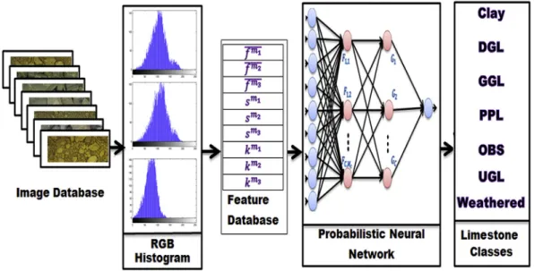
Many features can be extracted from an image that includes color, morphology, and textural features; however, it is not necessary that all features are signi_ficant for the speci_fic classi_fication purpose. Those redundant features increase the computational time expo-nentially for classification algorithms. Therefore, it is always neces-sary to extract limited features which could be helpful for classification. In this paper, color image histogram-based features were extracted. The reason for a color image histogram is that the content based image retrieval (Jadhav et al., 2012; Malik and Baharudin, 2013) and medical image analysis (Wiltgen et al., 2003), color image histogram feature plays an important role for classifi ca-tion. Medical image classification is considered to be a difficult task as it has a rich pattern in color and structure (Wiltgen et al., 2003). In the same way as medical image classification, limestone classification has a different pattern in color and structure; so it is expected that his-togram based features will capable to classify the limestone with better accuracy. The feature extraction method is shown in theFig. 1. The color histogram of an image has the ability to describe the frequency of the presence of a particular level of color. An image has mainly color feature; however, other features such as edges, textural, and morphological features can be derived from image color.

In this paper, three different histograms were calculated for each color space, red, green, and blue. The histogram was generated by scanning the red, green, and blue components of each pixel of the image.

Let, an imageIof sizepq, has a pixel intensityf(x,y), where

y) varies from 0 toL1 then the histogram can be calculated using (Gonzalez and Woods, 2002)

Hf ¼ N_f (1)

where,Nfrepresents the number of pixels in an image with

in-tensity levelf. From, histogram, three features, i.e. weighted mean, skewness, and kurtosis were extracted for all three color space.

The weighted mean of the color histograms was calculated to produce features that ensure the high intensity contributing higher than lower intensity. If the histogram of an imageIhas represented byH(f) and pixel intensityfvaries from 0 toL1, then weighted meanfwcan be calculated using

fw ¼ PL1 f¼0fHðfÞ PL1 f¼0f (2)

The skewness represents the spread of image pixel value from the mean value. Positive skewness represents the spread of pixel value more toward the right from mean, and negative skewness represents the spread of pixel value toward the left of the mean. The mean and variance is represented byfandv, and calculated as

f ¼ P_L1 f¼0fHðfÞ pq (3) v ¼ PL1 f¼0 ff2HðfÞ pq (4)

The skewness is calculated as

S ¼ 1 pq PL1 f¼0ðffÞ3HðfÞ ðpffiffiffivÞ3 (5)

The kurtosis represents the pixel value distribution along the mean. Kurtosis of histogram represented the height of the histo-gram. The kurtosiskis calculated as

k ¼ 1 pq PL1 f¼0ðffÞ4H f ffiffiffi v p 4 (6)

Figure 2.Architecture of Probabilistic Neural Network (PNN) for vision-based rock type classification. Figure 1.Feature extraction method adopted in this study.

Positive kurtosis represented a peaked distribution while negative kurtosis representedflat distribution.

The weighted mean, skewness, and kurtosis values were calculated in all three color space for all rock sample images. Altogether, total nine features were extracted from the rock im-ages. These features were then used as input for classification algorithms.

2.3. Probabilistic neural network (PNN)

Arti_ficial intelligence has been widely used to resolve a wide range of optimization, classification or prediction problems (Yaghouby and Ayatollahi, 2010; Yaghouby et al., 2010; Dong et al., 2014). Arti_ficial neural network (ANN) is a well-known branch of artificial intelligence which mimics the network structure of actual human brains. The main advantage of ANN lies in the fact that they areflexible models and can represent any non-linear relationship between input and output through appropriate training. In classification and regression, the network is presented with the input and output patterns for training, and given enough data and appropriate training, the network can be taught to recognize the relationship between input and output patterns. ANN has been applied to several real world classifi ca-tion (Yaghouby et al., 2009) and prediction problems (Kerh and Chu, 2002). PNN is a class of ANNs based on the well-known Bayesian classification (Specht, 1990; Goh, 2002).

In this paper, PNN was used as a classi_fier for rock-type classi-fication using the image features as input. A probabilistic neural network has similarity to back propagation model in the way they forwarded. But PNN has dissimilarity in learning procedure. The architecture of PNN had consisted of an input layer, pattern layer, summation layer, and the output layer. The pattern layer has sim-ilarity to radial basis network; however, summation layer has similarity to competitive network. The pattern layer has number of neurons same as input samples numbers and summation layer has the same number of neurons to target class. The architecture of PNN used in this paper is shown inFig. 2.

The input layer neurons take input from input vector

X ¼ ðfml

w ;Smi;kmiÞ,˛Rn,n¼9 wheremi¼(R,G,B) represents color

mapri¼1,2,3. These inputs had passed to the pattern layer where the neurons are divided into a number of classesC. The output of

thejth pattern neuroncth class had calculated using the following Gaussian Kernel: F_c;jX ¼ 1 2

ps

s

where,Xc;j˛Rnis the center of the kernel, and

s

spread (smoothing) parameter, determines the size of the receptive field of the kernel.

The summation layer of the network computes the approxi-mation of the conditional class probability functions through a combination of the previously computed densities,

Gc X ¼ X Nc j¼1 Fc;j X; c˛f1;2;.Cg (8)

where,Ncis the number of pattern neurons of classc, andwcjis

positive coefficient satisfying,PNc

j¼1wcj ¼1. Pattern vectorXhas

classified in the class corresponding to the summation unit with the maximum output,

OðXÞ ¼ argmax1cCðGCÞ (9)

The schematic diagram of the proposed methodology is pre-sented inFig. 3. The images are selected one after another and their features were extracted. These features were used to train the PNN network for classification.

3. Case study

3.1. Description of the study area

The study was carried out in a limestone mine in India, which supplied the raw materials for the captive cement plant. The area of the mine is more than 6 km2with a maximum reduced level of 444 m. The mine is covered with soil with some limestone out-crops. The study mine consists of nine different rock types, i.e. PPL (pink limestone), GGL (greenish gray limestone), DGL (dark gray limestone), LGL (light gray limestone), WTH (weathered lime-stone), UGL (upper gray limelime-stone), shale (SHL), clay, and

overburden soil (OBS). After blasting, the materials are either falling down next to the blast location or thrown to the furthest from the blast. Due to the movement of rock sample during blasting, rocks are formed heap like geometry after blasting and only some por-tions of rock samples can be visible from the surface. Therefore, an assumption is made in this study that the blasted rocks are distributed homogeneously and exposed surface of the blasted rocks are representative. The representative samples are collected from the freshly blasted face and study was carried out in the laboratory with a simulated environment. The stratified random sampling method was adopted where the rock samples were collected randomly from each rock-type with equal number of samples. This specific study was carried out in a part of the mine where only six rock-types, i.e. UGL, Clay, DGL, PPL, GGL, OBS, and WTH were exposed after blasting. Therefore, only these rock-types are considered for this study. A total 140 samples were collected from the mine with an approximate weight of 5 kg each. The size distribution of the collected rock samples was varied within the range of 2e8 cm.

3.2. Image acquisition and feature extraction

In this present work, all image acquisition experiments were carried out on a laboratory scale. The same experimental setup was used as presented inChatterjee et al. (2010). A digital camera (CX-7300, KODAK; Japan) was used for capturing the images from a fixed distance perpendicular to the base of the experimental setup. Images were captured in the experimental setup for all limestone rock samples those were collected from case study mine. A total number of ten consecutive images for each rock sample were captured by changing the orientation of the individual rock inside the experimental setup. From 140 rock samples, a total 1400 images were generated altogether. The images have a resolution of 0.15 mm/pixel in both horizontal and vertical directions. The im-ages acquired were 20801544 pixels in size.

A total number of nine features as discussed in Section2.2were then extracted from each of the individual images. These extracted features were used for the rock-type classification purpose.

3.3. Rock type classification using the probabilistic neural network

After extracting image features, the rock type classification was performed by probabilistic neural network model using image

features as input variables and rock type class as output variables. To see the effectiveness of the extracted image features and how the individual feature is different from others statistically, the mean comparison amongst the image features were performed. The ANOVA F-test was performed with a null hypothesis that means are equal. The ANOVA test results show that the null hypothesis can be significantly different at the 95% confidence level. Therefore, it can be concluded that all nine extracted image features have significant impact on rock-type classification.

To get further insight into this aspect, the box plots of the image features were prepared.Fig. 4presents the image feature-wise box plots. It is noted that a box-plot displays the data variation in a concise form by indicating the minimum, maximum, 1st quartile (25% of the data less than or equal to this value), 2nd quartile (50% of the data less than or equal to this value) and 3rd quartile (75% of the data less than or equal to this value) of an image feature. The distinguished pattern of image feature variations is clearly identi-fied through the box-plots. These results also provided some initial clues about why it is important to incorporate these image features for rock type classification.

All non-linear modeling algorithms, including probabilistic neural network require a separate data set for assessing the per-formance of the algorithm. Therefore, the available data were divided into two subsets: the training and the test. The classifi ca-tion models were developed on the training data set and their performances were measured on the test data set. In this paper, 75% of data (i.e. 1050) were used for training and remaining 25% of the data (i.e. 350) were used for testing purpose. The major concern related to data division is that of a valid model development these two data sets should have similar statistical characteristics; other-wise model might be trained with some data which has no rele-vance to the testing data. The data division was performed by randomly splitting the data into training and test sets; while monitoring the statistical properties of the two data sets. For verifying the statistical similarity of these two data sets, paired samplet-test was carried out. Thet-test results are presented in

Table 1and the results confirmed that these data sets are statisti-cally similar at 0.05 level of significance.Table 2shows the mean and standard deviation values of all nine image features for the training and the test data sets.

The training data were then used for developing the rock type classification model. The architecture of the probabilistic neural network model is _fixed. The network consisted of an input layer

Figure 4.Box plot for different images features (WMeanR, WMeanG and WMeanB are weighted mean for RGB; SkewR, SkewG and SkewB are skewness for RGB, KurtR, KurtG and KurtB are kurtosis for RGB).

containing nine image features, a pattern layer contains one neuron for each case in the training data set, a summation layer contains one pattern neuron for each rock type, and an output layer that compares the weighted votes for each rock type accumulated in the pattern layer and uses the largest vote to predict the target rock type. The Gaussian activation function was used for this study.

The training process of a PNN is essentially the act of deter-mining the value of the smoothing parameter. Traditionally, the value of this parameter was decided trial and error basis. However, it is noted that the smoothing parameter is the major influencing factor in probabilistic neural network model with a given set of data patterns. Smaller smoothing parameter value, PNN model acts as nearest neighborhood classification algorithm; whereas with higher value, PNN acts as matched filter. Therefore, selection of smoothing parameters and number of training data patterns is equally important for successful model developers. In selecting these two parameters, a grid search algorithm was adopted where smoothing parameter value varied from 1 to 10 and the numbers of training samples were varied from 0 to 1050 within an interval of 25.Fig. 5shows a 3-D surface plot of the correct classification. The effects of the smoothing parameter and the number of data pat-terns on the PNN output, therefore could easily be visualized from the plot. It has observed from the results that higher number of sample patterns and smaller value of spread produced better classification results.

Fig. 6 also provides a micro observation into the effect of smoothing parameter on the classification accuracy while main-taining the number of training patterns as 1050 as selected from the grid search algorithm. At this time, the smoothing parameter value varied from 0.01 to 1.1 and it was found that the smoothing parameter of 0.03 ensures maximum classification accuracy.

After training of the PNN network, it was tested with the test data set (350). The test data set consists of 50 samples each of all seven rock types.Table 3shows the confusion matrix of the test data results. The results revealed that the network satisfactorily classi_fied the rock types of the case study mine. The PNN satisfac-torily classified with more than 98% classification accuracy for clay, DGL, OBS, UGL, and weathered limestone; however classification accuracy of GGL and PPL rock samples are not up to that mark.

The result shows that for the GGL rock type, the misclassification error of 16% is almost the same as UGL. Only one sample of clay is misclassified as weathered limestone and one sample of OBS is mis-classified as clay. In case of weathered limestone, 2% were mis-classified as the PPL. On the other hand, there was no misclassifi -cation for the DGL rock-type. Only one UGL sample was mis-classified as the DGL.

On the contrary, a large number of GGL samples (8) were mis-classified as DGL. To understand the reason of such large misclas-sification, an analysis was carried out using these 8 samples and rest 42 GGL samples. Thet-test was performed for all selected nine

Table 1

Paired samplet-test between training and test data set. Parameter Feature fm1 w fwm2 fwm3 Sm1 _Sm2 _Sm3 _km1 _km2 _km3 t-statistics 0.102 0.183 0.466 0.655 0.652 0.648 0.485 0.728 0.156 p-value 0.9187 0.8545 0.6407 0.5126 0.5144 0.5169 0.6273 0.4664 0.8756 Standard error 3.2275 2.3051 7.4269 0.2560 0.2902 0.4210 0.3090 0.2646 0.5601 Table 2

Mean and standard deviation values for the training and the test data sets for all nine features.

Parameter Feature

fm1

w fwm2 fwm3 Sm1 Sm2 Sm3 km1 km2 km3

Mean Train 40.397 38.133 27.003 0.468 0.357 0.097 3.082 2.944 3.234

Test 40.418 38.16 26.789 0.457 0.345 0.080 3.0733 2.932 3.229

Standard deviation Train 3.188 2.290 7.452 0.253 0.287 0.419 0.312 0.265 0.555

Test 3.340 2.349 7.349 0.265 0.299 0.426 0.3 0.265 0.575

features of those two groups of samples, i.e. one group with 8 GGL samples and another group with 42 GGL samples. It was observed from the results that the means are significantly different for 6 image features out of 9 features. A significant difference of 6 fea-tures in these 8 samples might be the reason of their misclassifi -cation. However, when thet-test was performed for checking the mean difference between these 8 GGL samples and 50 DGL samples for all 9 features, it was observed for at least 8 features their means are not significantly different. This is the main reasons why these 8 GGL samples were misclassified as DGL. Also, visual observation confirmed that there is some intrusion of DGL rocks in these 8 GGL samples.

The large number of misclassification was also observed for PPL rock type; where 4 samples are misclassified as DGL, 2 samples are misclassi_fied as GGL, and 4 samples are misclassi_fied as UGL. Thet -test results confirmed that the mean value of these 10 samples is significantly different from the mean value of the rest of the 40 PPL rock samples. Further, visual inspection established the fact that some mixing of other rock types, especially DGL, GGL, and UGL, were taking place with these 10 PPL rock samples.

To confirm the ability of the proposed classification method, four indices like sensitivity, specificity, misclassification and accu-racy were calculated from the confusion matrix.Table 4represents the value of these four parameters for all seven rock types. The highest value of sensitivity, specificity, and accuracy (i.e. 1) and the

lowest value of misclassi_fication (i.e. 0) represent the perfect clas-sification results. Therefore, it is desirable for a good classification model to have high sensitivity, specificity, accuracy values along with low misclassification value. It is clearly observed from table that the performance of a classification model is satisfactory. The overall classification accuracy of the proposed classification model is very high (94%), where only 22 rock samples are misclassified out of test samples.

4. Comparative study

The performance of the PNN classification model was compared with Learning Vector Quantization (LVQ) (Kohonen, 1990), Classi-fication Tree (Breiman et al., 1984), and Naïve Bayes Classifier (Gose et al., 1996) for all seven rock types. The learning vector quantiza-tion model was developed using nine image features as input and rock type class as output. The learning rate and number of hidden nodes were selected by trial and error method. The classification tree was developed using an iterative process with Gini’s diversity index (Breiman et al., 1984) as an optimization criteria. For Naïve Bayes Classifier, the conditional probability distributions were calculated assuming all nine image features following Gaussian distribution. The four classification parameter sensitivity, speci-ficity, misclassi_fication and accuracy had calculated for each class of limestone using these classifiers and the results are presented in

Table 5. It is observed from the table that for the clay, GGL, PPL, UGL, and weathered limestone all four parameter values using the pro-posed algorithm are better than all three algorithms. However, for the DGL, specificity value is better using LVQ algorithm, and for OBS, the sensitivity value is better using the LVQ algorithm. How-ever, overall, the proposed algorithm is outperforming other three algorithms for all seven rock types.

5. Conclusion

A PNN model was developed for rock type classification of limestone using different image features. The computer vision-based study was conducted within a controlled environment in the laboratory scale for identifying the rock types. All rock images were captured at a constant distance from the top of the rock surface and features are extracted from these images. A total number of 9 histogram based features were extracted from each and individual image.

The developed model was validated using a test data set. The results demonstrated that the misclassification error is relatively very less within 5e6%. The results also showed that the

misclassi-fication error is significantly very less in case of clay, DGL, OBS, UGL, and weathered limestone rock types; whereas, the DGL and PPL produced relative large misclassification error (16e20%). The

re-sults from this study also indicated the usefulness of vision-based rock type classification of the limestone. A comparative study with other three classifiers reveals that the developed PNN model performed better than these classifiers for classification of lime-stone rocks.

Figure 6.Classification accuracy of rock type with different spread values in PNN model.

Table 3

Confusion matrix for the seven rock type classification. Original Classified

Clay DGL GGL PPL OBS UGL Weathered

Clay 49 0 0 0 0 0 1 DGL 0 50 0 0 0 0 0 GGL 0 8 42 0 0 0 0 PPL 0 4 2 40 0 4 0 OBS 1 0 0 0 49 0 0 UGL 0 1 0 0 0 49 0 Weathered 0 0 0 1 0 0 49 Table 4

Classification parameter for testing limestone samples.

Parameter Class

Clay DGL GGL PPL OBS UGL Weathered

Sensitivity 0.9800 1.0000 0.8400 0.8000 0.9800 0.9800 0.9800

Specificity 0.9967 0.9567 0.9933 0.9967 1.0000 0.9867 0.9967

Misclassification 0.0057 0.0371 0.0286 0.0314 0.0029 0.0143 0.0057

The main limitation of this study is that the classification was performed the whole rock samples where multiple rocks are pre-sent. Therefore, the algorithm will be working perfectly well when rock type of all rocks in a specific sample is same. However, the proposed algorithm can easily be extended for classifying different types of rock from the same sample, by applying an image seg-mentation algorithm and classifying individual rocks from an im-age than the whole imim-age. Also, the study was conducted at a laboratory scale by collecting samples from limestone mine. To apply the proposed method in the real miningfield, the same image acquisition setup, camera, and image features can be used in larger scale to get similar results. After identifying the correct rock type, one can correctly plan the blending sequences to send desire quality of materials to the cement plant.

References

Breiman, L., Friedman, J.H., Olshen, R.A., Stone, C.J., 1984. Classification and Regression Trees. Wadsworth, California, USA.

Casali, G., Vallebuona, C., Perez, G., Gonzalez, R., Vargas, L., 2000. Lithological composition and ore grindability sensors, based on image analysis. In: Pro-ceedings of the XXI International Mineral Processing Congress, pp. 9e16. Rome, A1.

Chatterjee, S., 2013. Vision-based rock-type classification of limestone using multi-class support vector machine. Applied Intelligence 39, 14e27.

Chatterjee, S., Bhattacherjee, A., 2011. Genetic algorithms for feature selection of image analysis-based quality monitoring model: an application to an iron mine. Engineering Applications of Artificial Intelligence 24 (5), 786e795.

Chatterjee, S., Bhattacherjee, A., Samanta, B., Pal, S.K., 2010. Image-based quality monitoring system of limestone ore grades. Computers in Industry 16, 391e408.

Dong, Z., Duan, S., Hu, X., Wang, L., Li, H., 2014. A novel memristive multilayer feedforward small-world neural network with its applications in PID control. The Scientific World Journal 394828 (1e12).

Duda, R.O., Hart, P.E., 1973. Pattern Classification and Scene Analysis. Wiley, New York, p. 512.

Goh, A.T.C., 2002. Probabilistic neural network for evaluating seismic liquefaction potential. Canadian Geotechnical Journal 39 (1), 219e232.

Gonzalez, R.C., Woods, R.E., 2002. Digital Image Processing. Prentice Hall, Upper Saddle River, New Jersey, p. 797.

Gose, E., Johnsonbaugh, R., Jost, S., 1996. Pattern Recognition and Image Analysis. Prentice-Hall, Upper Saddle River, NJ, p. 484.

Ingram, K.D., Daugherty, K.E., 1991. A review of limestone additions to Portland cement and concrete. Cement and Concrete Composites 13 (3), 165e170. Jadhav, D., Phadke, G., Devane, S., 2012. Adaptive color segmentationda

compari-son of neural and statistical methods. In: Proceedings of the Second Interna-tional Conference on Computer Science, Engineering and Application (ICCSEA), pp. 101e111. New Delhi, India.

Kerh, T., Chu, D., 2002. Neural networks approach and microtremor measurements in estimating peak ground acceleration due to strong motion. Advances in Engineering Software 33, 733e742.

Khorram, F., Memarian, H., Tokhmechi, B., Soltanian-zadeh, H., 2012. Limestone chemical components estimation using image processing and pattern recog-nition techniques. Journal of Mining & Environment 2, 126e135.

Kohonen, T., 1990. Improved versions of learning vector quantization. In: Interna-tional Joint Conference on Neural Networks IJCNN, pp. 545e550. San Diego, California, I.

Lea, F.M., 1971. The Chemistry of Cement and Concrete. Chemical Publishing Company, New York 1092.

Lepisto, L., Kunttu, I., Visa, A., 2005. Rock image classification using color features in Gabor space. Journal of Electronic Imaging 14, 040503.

Malik, F., Baharudin, B., 2013. Analysis of distance metrics in content-based image retrieval using statistical quantized histogram texture features in the DCT domain. Journal of King Saud UniversityeComputer and Information Sciences 25, 207e218.

Mayfield, L.L., 1988. Limestone additions to Portland cementdan old controversy revisited. Cement Concrete and Aggregates 10 (1), 3e8.

Micheletti, N., Foresti, L., Robert, S., Leuenberger, M., Pedrazzini, A., Jaboyedoff, M., Kanevski, M., 2014. Machine learning feature selection methods for landslide susceptibility mapping. Mathematical Geosciences 46 (1), 33e57.

Mukherjee, D.P., Potapovich, Y., Levner, I., Zhang, H., 2009. Ore image segmentation by learning image and shape features. Pattern Recognition Letters 30, 615e622.

Murtagh, F., Starck, J.L., 2008. Wavelet and curvelet moments for image classifi ca-tion: application to aggregate mixture grading. Pattern Recognition Letters 29 (10), 1557e1564.

Narendra, P.M., Fukunaga, K., 1977. A branch and bound algorithm for feature se-lection. IEEE Transactions on Computers 26, 917e922.

Oestriech, J.M., Tolley, W.K., Rice, D.A., 1995. The development of a color sensor system to measure mineral compositions. Minerals Engineering 8, 31e39. Perez, C.A., Estévez, P.A., Vera, P.A., Castillo, L.E., Aravena, C.M., Schulz, D.A.,

Medina, L.E., 2011. Ore grade estimation by feature selection and voting using boundary detection in digital image analysis. International Journal of Mineral Processing 101, 28e36.

Singh, V., Rao, S., 2006. Application of image processing in mineral industry: a case study of ferruginous manganese ores. Mineral Processing and Extractive Met-allurgy 115, 155e160.

Specht, D.F., 1990. Probabilistic neural networks. Neural Networks 3, 109e118. Steppe, J.M., Bauer Jr., K.W., Rogers, S.K., 1996. Integrated feature and architecture

selection. IEEE Transactions on Neural Networks 7, 1007e1014.

Tessier, J., Duchesne, C., Bartolacci, G., 2007. A machine vision approach to on-line estimation of run-of-mine ore composition on conveyor belts. Minerals Engi-neering 20, 1129e1144.

Wiltgen, M., Gerger, A., Smolle, J., 2003. Tissue counter analysis of benign common nevi and malignant melanoma. International Journal of Medical Informatics 69 (1), 17e28.

Yaghouby, F., Ayatollahi, A., 2010. An arrhythmia classification method based on selected features of heart rate variability signal and support vector machine-based classifier. In: Proceedings of International Federation for Medical and Biological Engineering (IFMBE) 25/IV, pp. 1928e1931. Munich, Germany.

Yaghouby, F., Ayatollahi, A., Soleimani, R., 2009. Classification of cardiac abnor-malities using reduced features of heart rate variability signal. World Applied Sciences Journal 6, 1547e1554.

Yaghouby, F., Ayatollahi, A., Bahramali, R., Yaghouby, M., HosseinAlavi, Amir, 2010. Towards automatic detection of atrialfibrillation: a hybrid computational approach. Computers in Biology and Medicine 40, 919e930.

Table 5

Comparison of PNN network with three different classifiers using four classification parameters.

Parameter Class

Clay DGL GGL PPL OBS UGL Weathered

Sensitivity PNN 0.9800 1.0000 0.8400 0.8000 0.9800 0.9800 0.9800 LVQ 0.5800 0.2400 0.6600 0.7800 1.0000 0.9200 0.8000 C-Tree 0.8200 0.9000 0.8200 0.7000 0.9600 0.8600 0.8000 Naïve Bayes 0.7000 0.3200 0.8200 0.4400 0.9200 0.9200 0.8400 Specificity PNN 0.9967 0.9567 0.9933 0.9967 1.0000 0.9867 0.9967 LVQ 0.9767 0.9800 0.9400 0.9300 0.9500 0.9467 0.9400 C-Tree 0.9667 0.9467 0.9867 0.9700 0.9900 0.9867 0.9633 Naïve Bayes 0.9833 0.9233 0.9200 0.9267 0.9967 0.9733 0.9367 Misclassification PNN 0.0057 0.0371 0.0286 0.0314 0.0029 0.0143 0.0057 LVQ 0.0800 0.1257 0.1000 0.0914 0.0429 0.0571 0.0800 C-Tree 0.0543 0.0600 0.0371 0.0686 0.0143 0.0314 0.0600 Naïve Bayes 0.0571 0.1629 0.0943 0.1429 0.0143 0.0343 0.0771 Accuracy PNN 0.9943 0.9629 0.9714 0.9686 0.9971 0.9857 0.9943 LVQ 0.9200 0.8743 0.9000 0.9086 0.9571 0.9429 0.9200 C-Tree 0.9457 0.9400 0.9629 0.9314 0.9857 0.9686 0.9400 Naïve Bayes 0.9429 0.8371 0.9057 0.8571 0.9857 0.9657 0.9229