Improving time–frequency domain sleep EEG classification via singular spectrum analysis

(1)

1

Improving Time-Frequency Domain Sleep EEG Classification via Singular Spectrum

Analysis

Sara Mahvash Mohammadia,∗_{, Samaneh Kouchaki}b_{, Mohammad Ghavami}a_{, Saeid Sanei}b a_{Department of Engineering and Design, London South Bank University,London, UK}

b_{Faculty of Engineering and Physical Sciences, University of Surrey, Guildford, UK}

Abstract

Background: Manual sleep scoring is deemed to be tedious and time consuming. Even among automatic methods such as Time-Frequency (T-F) representations, there is still room for more improvement.

New method: To optimise the efficiency of T-F domain analysis of sleep electroencephalography (EEG) a novel ap-proach for automatically identifying the brain waves, sleep spindles, and K-complexes from the sleep EEG signals is proposed. The proposed method is based on singular spectrum analysis (SSA). The single-channel EEG signal (C3-A2) is initially decomposed and then the desired components are automatically separated. In addition, the noise is removed to enhance the discrimination ability of features. The obtained T-F features after preprocessing stage are classified using a multi-class support vector machines (SVM) and used for the identification of four sleep stages over three sleep types. Furthermore, to emphasize on the usefulness of the proposed method the automatically-determined spindles are parameterised to discriminate three sleep types.

Result: The four sleep stages are classified through SVM twice: with and without preprocessing stage. The mean accuracy, sensitivity, and specificity for before the preprocessing stage are: 71.5±0.11%, 56.1±0.09% and 86.8±0.04% respectively. However, these values increase significantly to 83.6±0.07%, 70.6±0.14% and 90.8±0.03% after applying SSA.

Comparison with existing method: The new T-F representation has been compared with the existing benchmarks. Our results prove that, the proposed method well outperforms the previous methods in terms of identification and represen-tation of sleep stages.

Conclusion: Experimental results confirm the performance improvement in terms of classification rate and also repre-sentative T-F domain.

Keywords: Electroencephalogram, Feature extraction, Sleep, Singular spectrum analysis, Time-Frequency representation

1. Introduction

Sleep research has applications in medical science, psy-chology, and bioengineering. Amongst different sleep dis-orders such as sleep apnoea, insomnia and narcolepsy, many of them divulge themselves through sleep disturbances like

5

depression and schizophrenia [1]. Sanitising and study-ing sleep can be accomplished through polysomnographic (PSG) measurements, encompassing EEG, electromyogram (EMG), and electrooculogram (EOG) [2]. The Rechtschaf-fen and Kales standard (R&K) [3] and American Academy

10

of Sleep Medicine (AASM) [4] are commonly used to guide-line, regulate, and govern the standards for classifying and monitoring the sleep stages. R&K described the sleep as a six sequence stages including: awake, stage 1, stage 2, stage 3, stage 4 , and rapid eye movement (REM). Stages

15

1, 2, 3, and 4 are categorised under non-rapid eye move-ment (NREM). However, sleep stages 3 and 4 are recently

∗_{Corresponding author}

grouped into one stage by AASM and assigned N3 stage. Thus, NREM sleep is divided into three stages: N1, N2, and N3.

20

Generally speaking, awake stage is observed at the start of the sleep and is known as a shift stage from complete awareness to a half-sleepy condition. This stage is charac-terised mainly by its frequency range of 8 to 12 Hz that contains alpha rhythms, eye movements, and high muscle

25

tone. Stage N1 is referred to as a moving stage from wake-fulness to sleep. This stage entails a low-voltage, mixed frequency EEG tracing accompanied by high amplitude theta waves. It is as short as 5−10 minutes. Stage N2 is known as sleep baseline and lasts for approximately 20

30

minutes. This stage can be identified by the incidence of sleep spindles and K-complexes. Sleep spindles are bursts of rapid rhythmic brain wave activity which appear within the frequency range of 12−14 Hz and last for approxi-mately 0.5 second. K-complex is an abrupt peak in time

35

that spreads in frequency domain [5].

(2)

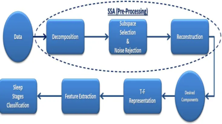
Figure 1: Block diagram of the proposed sleep scoring approach.

activity (SWA) with frequencies up to 2 Hz and amplitude of more than 75 µV. At this stage spindles may be gen-erated. However, the amount of sleep spindles decrease

40

as the sleep deepens. 17−20% of the total sleep time is in stage N3. This stage is also called as slow wave sleep (SWS) Following the NREM stages, REM sleep stage cor-responds to dreaming and contributes to 20−25% of a normal sleep. It is defined as an occurrence of rapid eye

45

movement under closed eyelids [6].

Study of sleep stages has gained appreciation from the researchers. This is because of the fact that different sleep disorders and sleep deprivation impact on individuals as well as public health to the large extend [7]. Manual sleep

50

stage classification and scoring is performed by experts and clinicians. However, this method is subject to hu-man error. Moreover, the hu-manual method is a very te-dious and arduous exercise which leads to a low reliabil-ity and high subjective error [8]. In order to effectively

55

tackle this problem different automatic classification of sleep stages based on multi-channel EEG signals [9][10] or single-channel EEG signal [11][12] are highly desired.

Automatic sleep detection is an active area in research. Nonetheless, T-F methods compared with other techniques

60

have received more attention due to existing clear T-F pat-terns in sleep EEG. Most of the solutions for sleep EEG analysis like Fourier transform are only capable of pro-viding generic frequency specification while the transient events are not discussed explicitly. Wavelet transform

65

(WT) is another technique for sleep analysis. However, there are a couple of drawbacks associated with WT in-cluding dependency of its results to the choice of mother wavelet and also the fact that the wavelet basis functions are not data dependent. In addition, unlike Fourier

trans-70

form which only exploits sinusoid functions or in case of wavelet transform which uses mother wavelet, matching pursuit(MP) benefits from a large dictionary size which gives high flexibility in signal structure identification and parameterizations and better deals with nonstationarity of

75

the signals. [13].

For years, different T-F representation methods have been used for automatic sleep stage classification [12, 14, 15]. However, these methods are impacted by interferences

stemmed from unwanted components. Durka in [16]

pro-80

posed automatic detection and parametrization of sleep events on the premise of MP spectrum. However, in stage N3 the alpha wave totally vanishes and non-frequent low amplitude spindles may occur. The spindles have fre-quency within alpha range but usually occur in the absence

85

of normal brain alpha wave. In addition, the key compo-nents for classifying the sleep stages are brain waves, sleep spindles, and K-complexes. In the T-F energy map for various sleep stages in [16] all components including de-sired and undede-sired are plotted. Hence the purpose of this

90

paper is to append a preprocessing stage to address these issues.

Singular spectrum analysis (SSA) method is leveraged for automatic identification and extraction of desired com-ponents: brain waves, spindles and K-Complex in their

95

actual locations. SSA has had emerging application in trend extraction, time series decomposition, periodicity extraction, signal extraction, noise reduction, and filtering [17, 18]. In time series analysis, SSA plays a major role as a robust technique for tackling a diverge range of issues

100

in practice. Recently, in terms of biomedical signal pro-cessing application, SSA has been used for restoration of heart sound from lung sound [19], and separating ECG and EMG [20]. It has been also considered for estima-tion of detailed gait analysis and parameters from

105

a wearable devices [21]. More recently,SSA has been employed in signal processing applications such as processing of multichannel EEG signals for classification of five sleep stages [9] and evaluation of alpha and delta waves for more accurate determination of the transition

110

between two sleep stages [22].

This paper describes the extraction of desired compo-nents from EEG signals prior to applying T-F transform and classification. The overall strategy of this work is il-lustrated in Figure 1. Note that the EEG sleep signals are

115

deemed to have nonstationarity. SSA benefits from the elements of classical time series analysis, linear algebra, multivariate geometry, multivariate statistics, dynamical systems, and signal processing, and can exploit the signal nonsstationarity [17]. In addition, the noise component

120

can be removed during the SSA decomposition. This is envisaged to be another significant merit of SSA as a pre-processing stage.

Here, a new constrained SSA has been proposed. Then, the extracted features from both methods i.e. with and

125

without preprocessing stage, were classified with the aid of the support vector machine (SVM) classifier. Classi-fication accuracy of awake, N1+ REM, N2, and SWS is improved through using SSA preprocessing.

In this work, SSA is applied to sleep EEG

130

analysis. In another study, pulse oximetry and heart rate sensors are employed in order to diag-nose sleep disorders [23]. Therefore, as a future work, the current application can be improved by incorporating the joint motion [21], heart rate, and

135

(3)

Sleep EEG in the course of NREM is characterised with sleep spindles. The degree of hyperpolarization of thalamocortical cells (TC) justifies the given fluctuations and the causing method. With the aid of fast Fourier

140

transform (FFT), spectral analysis of the NREM displays frequency specific modulation of spindle frequency activ-ity which varies based on the homeostatic sleep pressure [24][25]. Hence as another SSA application, through pa-rameterising the automatically extracted sleep spindles,

145

we also focus on the impact of different sleep types on the extracted spindles characteristics. In other words, the effect of enhanced sleep pressure after sleep deprivation (SD) and low sleep pressure after sleep extension (SE) on spindle characteristics is analysed using mean amplitude,

150

density (i.e. the number of sleep spindles per 20 seconds epoch), duration, and frequency. After that, the spindles’ features are employed as an input to the SVM classifier to classifynormal sleep(SN), SE, and SD.

The rest of this paper is organised as follows: section 2

155

overviews the fundamentals of the employed method. Sec-tion 3 reveals the experimental results obtained and and discuss the results. Finally, the last section draws the con-cluding points.

2. Materials and Methods

160

2.1. Matching Pursuit

MP has been introduced by Mallat and Zhang in [26]. MP application is based on adaptive delineation of signal (y) with functions selected from a wide collection of wave-forms, known as dictionary (F). In the initial stage, the waveform that best fits the signal (fγ0) is selected from the

dictionaryF. Then, in each iterationnwe have [16]:

       R0y=y f ∈H Rn_y₌_h_Rn_y_,_f γnifγn+Rn+1y fγn= arg max fγi fγi∈F|hR n_y_,_f γii| (1)

Let H be the Hilbert space. fγn and Rny are the

wave-form matched to the signal and the remaining signal after each iteration respectively andhRn_y_,_f

γnirefers to

cross-correlation. The perfect signal approximation is achieved in an infinite number of iterations. Nonetheless, practi-cally, a few number of waveforms (after finite number of iterations) result in a good signal approximation.

y= M X n=0 hRny,fγnifγn= M X n=0 anfγn (2)

whereMis the total number of iterations. Functionsfγare

selected from dictionary of the Gabor functions. Gabor is the best filtering in the T-F domain and can provide the optimal T-F localization using the complete Dirac and Fourier bases [16]. Real valued continuous time Gabor functions are shown as:

fγ(t) =N(γ)e−π( t−u

s ) 2

cos(ω(t−u) +ϕ) (3)

whereN(γ) is a normalising factor offγ andλ={u, ω, s}

corresponds to the parameter of the Gabor function (trans-lating, modu(trans-lating, and scaling). T-F distribution of the energy of the signal can be driven from expansion (2). Hence, the Wigner distributions W of the chosen func-tion are added while the cross-terms are removed so that [26][16]: ey(t, ω) = M X n=0 |hRny,fγni|2Wfγn(t, ω) = M X n=0 a2_nWfγn (4)

whereey is the T-F distribution. 2.2. Singular Spectrum Analysis

SSA works based on how well the diverged components can be taken apart from each other [20]. The

fundamen-165

tal SSA approach entails two stages which complement each other; decomposition and reconstruction. Each of these two stages, in turn, encompasses two distinct stages. The first stage involves embedding accompanied by singu-lar value decomposition (SVD) to decompose the signal.

170

Stage two consisting of grouping and diagonal averaging, reconstruct the signal while exploiting it for further anal-ysis .

2.2.1. Decomposition

In the case of basic univariate SSA, a time series f

should be mapped into a matrix known as trajectory ma-trix: X= [x1, . . . ,xn] = (xij)l,ni,j=1 =      f1 f2 f3 ... fn f2 f3 f4 ... fn+1 .. . ... . .. ... fl fl+1 fl+2 ... fs      (5)

with one-dimensional vectors xi = [fi, fi−2, . . . , fi+l−1]T,

wheren=s−l+ 1 andl is the window length (1< l < s). Note that, the window lengthlshould be adequately large to cater the information about the data variation. It is evident from (5) that the trajectory matrix is a Han-kel matrix where the diagonal elements (i+j= const) are equal [17, 27].

Following the previous stage, SVD is performed to de-compose the trajectory matrix into its eigen subspaces. To this end, consider the covariance matrix Cx = XXT

with eigenvalues λ1, λ2, . . . , λl in the decreasing order (λ1> λ2> . . . > λl) andq1, q2, . . . , qlcorresponding eigen-vectors; therefore, SVD of the trajectory matrix can be rewritten as: X=X1+X2+. . .+Xr (6) wherevj =XTqj/ p λj,Xj= p λjqjvjT, and

(4)

The set (λj,qj,vj) is named the j-th eigentriple of the

175

matrix X. The definition of Xj is equivalent to the

ele-mentary matrix. Projecting a time series onto each eigen-vector yields the corresponding temporal principal compo-nent (PC) [19, 28].

2.2.2. Reconstruction

180

In the initial step of reconstruction stage, the elemen-tary matricesXj are splitted into several groups and then

the matrices within each group are summed [17]. There-fore, each group is displayed by the related matrix ˜Xg ⊂

Rl×n where: X= gt X g=1 ˜ Xg (8)

in which, ˜Xgrepresents the sum of the elementary matrices

within the groupg,gtspecifies the total number of groups,

and index g refers to the g-th subgroup of eigentriples. After completing the split stage, a specific ( ˜Xg) is chosen

and then Hankelization procedure (averaging along entries with indices i+j = const) reconstructs the subseries. In this case if ˜xij points to an element of the matrix ( ˜Xg), k-th term of the new reconstructed series ˜xij is computed by making the average of all along all i, j in a way that (i+j =k+ 1). Therefore, the following parameters can be initialized as k = 1, ˜f1 = ˜x11 and for k = 2, ˜f2 = (˜x12+ ˜x21)/2 and so on [17]. ˜ Xg=      ˜ x11 ˜x12 . . . x˜1,n ˜ x21 ˜x22 . . . x˜2,n+1 .. . ... . .. ... ˜ xl,1 xl,l˜ +1 . . . xl,s˜      ˜ f = [ ˜f1,f˜2, . . . ,f˜s] (9)

where ˜findicates the reconstructed time series with length

s. Note that one of the major problems in SSA is to find an appropriate group of eigentriples in order to reconstruct the desired component [29].

2.3. Constrained SSA

185

In order to extract the EEG periodic signals such as spindles, alpha, theta, and delta the following constrains can be applied:

I. Subspace Rejection; Each eigenvalue in the decompo-sition stage represents the variance of the signal in the direction of the corresponding PC. Eigenvalues related to the more powerful signals are located in the lower spaces whereas less powerful signals occur in higher sub-spaces where the noise components usually arise. There-fore, the lower subspace is desirable here. To separate the lower subspace from the noise part, the following crite-rion should be applied to remove the noise part . All the PCs associated with the eigenvalues above 90% of the to-tal variance of the signal (i.e. the sum of all eigenvalues

equals the total variance of the original time series) are omitted. Eigenvalueλj is rejected ifj >L, where [19]:

L= min ( h: Ph i=1λi Pl i=1λi >0.9 ) (10)

h is defined as the number of eigenvalues whose overall energy is 90% of the total energy.

II. Periodic Component Extraction; a pseudo-periodic time series is factorised into some eigenvalue pairs using SSA [30, 28]. Since the objective of this section is to extract

190

the oscillatory components (i.e. sleep spindle, delta, theta, and alpha), the periodicity nature of these components is used here to choose the best subgroup of PCs for recon-struction of the brain waves. Thus, using the lower sub-space indicated in the former subsection, only eigenvalues

195

appeared as pairs are selected.

Following equation (7) and [17], the best subgroup of

X is selected by minimisation of k X−X(d) _k

F where

F stands for Frobenius norm andkXk2

F=

Pr

j=1λj and

λj =k Xj k2F for j = 1,· · · , r. The ratio λj/kXj k

2 is

200

therefore the contribution of the trajectory matrix gener-ated by the corresponding eigentriple (p

λj,qj,vj).

How-ever, the following points are important for the eigenvalue pairs selection [19, 28]:

• The possibility that the selected eigenvalue pairs

be-205

long to noise components.

• The possibility of having two equal eigenvalues is low mainly due to noise effect.

Therefore, in order to acquire the actual periodic pair, the eigenvalue pairs λj andλi are chosen as a pair only if all

210

of the following circumstances are satisfied:

i. iandjare less thanL, whereLis defined in (10) to dis-cards all eigenvalues assumed to be associated with noise

where the value ofKcan be changed according to the wave-forms amplitude. Hence, a specificK value is set for each PC. Alpha, theta, and delta contain higher amplitudes than spindles. Therefore, according to what was discussed earlier, since their eigenvalues are within the lower

sub-220

spaces, higher thresholds are chosen for them(K= 0.05). On the other hand, for spindles with lower amplitudes, the eigenvalues are skewed towards right and thus a lower value forK is selected(K= 0.005). If no eigenvalue pairs are obtained, it simply means that the component does

225

not exist in the given time domain signal [28]. However, if some eigenvalues is chosen, the highest peak in the Fourier transform of the associated eigenvectors is relevant to the frequency of the periodic component [31]. Therefore, the power spectrum density is used to estimate the related

230

frequency. The peak is required to fall into the desired frequency range (i.e. spindles (12-16 Hz), alpha (8-12 Hz), theta (4-7 Hz), and SWA (1-4 Hz)).

(5)

K-complex has a different structure compared to spin-dles and other mentioned sleep EEG waves. It abruptly

235

appears in the EEG signal with larger amplitude in a shorter period of time. Subsequently, the extraction of K-complex is relatively easy. The distribution of this wave-form has a greater kurtosis than the rest of the EEG signal. As a result, seeking the highest kurtosis, the summation

240

of the signals reconstructed from a group of eigenvalues and their associated eigenvectors constitute the detection of K-complex.

Parameter Settings: The size of embedding windowl (num-ber of columns of trajectory matrix) should make a

com-245

promise between low computational complexity and infor-mation quality. The embedding window should be suffi-ciently large to capture at least one period of the expected periodic signal. In addition, it has been suggested that

l should not be more than n/2 [17]. Window length is

250

also selected based on the lowest frequency of interestF w

(l >=F w_{F s}) [19]. Therefore, by settingl to 200, more than two cycles of the oscillatory components are covered by the window (Fs=sampling frequency of 256 Hz).

2.4. Feature Extraction

255

SSA is applied to the EEG signal for decomposing each 10 second segment into different frequency bands. Pre-cise representation of the sleep EEG commonly demands for the localization of signal structure in time and fre-quency simultaneously. Therefore, appropriate temporal

260

and spectral features are extracted from the EEG signals in different frequency ranges. These statistical descriptors are then used as the inputs to the classifier for classifica-tion purpose:

• Mean of absolute power in different frequency bands

265

described as follows:

Mean Absolute Power Frequency Bands

P1 K-complex (0.5-1.5 Hz)

P2 Delta (1.5-4 Hz)

P3 Theta (4-8 Hz)

P4 Alpha (8-12 Hz)

P5 Sleep Spindle (12-16 Hz)

• Sum of power in all frequency bands: P6

• Mean and standard deviation of ratios includingP1,

P2, P3, P4, andP5 divided byP6 produce 12 fea-tures.

270

• Mean and standard deviation of P1+_P₆P2 (delta activ-ity),

• Mean and standard deviation of P_P4₆ (alpha activity),

• Mean and standard deviation of P1+_P₆P5 (K-complex and sleep spindle), [15]

275

• Mean and standard deviation of ratios: P4

P2+P3, P3 P2+P4, P2 P3+P4 [32]. 2.5. Multiclass SVM classification

In a review of classification algorithms for EEG signals the performances of K-nearest neighbor (KNN), SVM, and

280

linear discriminant analysis (LDA) have been compared [33]. Based on this study, they recommended an SVM classifier for this purpose. SVM has also been previously used for classification of sleep stages [34, 35].

The nature of SVMs are based on binary classification

285

algorithms [17]. In case of linearly-separable data, SVM attempts to construct optimum hyperplane separating the training samples and the decision boundaries. Hyperplane construction whereby vT_x₊_b _{= 0 (}_v _{represents the}

hy-perplane coefficients vector and bias term is notated by b)

290

in a way that the margin between the hyperplane and the nearest point is magnified to the maximum in a way which can fit into the quadratic-optimization problem [36].

In case of linearly-inseparable data, the support vec-tors are taken into consideration and mapped to a high

di-295

mensional space in the hope that a segregating hyperplane can be detected. Kernel function is a nonlinear mapping function. Four common kernel functions include: linear, polynomial, radical basis function (RBF), and sigmoid. Finding the appropriate kernel differs for each problem.

300

Nonetheless, the RBF kernel is extensively employed which forms the cornerstone of the current research as well. Generally, the development of SVMs are for two-classes classification problems. However, the aim of this work is to automatic discrimination between four classes (awake,

305

N1 + REM, N2, and SWS). For this objective, the design of multiclass SVM with a ”one–against–all” approach is implemented.

3. Results and Discussion

In this paper, in order to to accentuate the usage of

310

SSA as a preprocessing step for sleep events detection, MP time-frequency representation is employed. MP has been used to compare the effect of preprocessing data on the T-F representation. The results prove that by using SSA as the method in the preprocessing stage, better

represen-315

tation and identification of the desired signal components can be achieved. The ultimate goal of the current work is to automatically classify the sleep stages. Therefore, the preprocessed data is used for feature extraction and then classification. This work concentrate on two stages;

320

classifying different sleep stages and different sleep types. Hence, the following subsection show firstly the results of applying the proposed method on real data and T-F map of energy of these data. Next, the classification of sleep stages are provided and the results compared with those

325

of raw data. Finally, the classification of sleep types is presented.

(6)

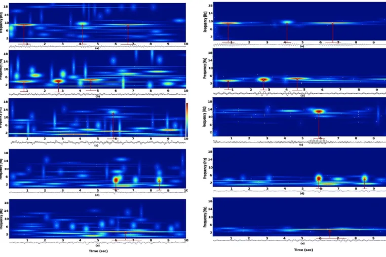
Figure 2: T-F representation of different sleep EEG stages for 10s segment; (a) awake, (b) N1, (c) N2, (d) N2, and (e) SWS.

3.1. Data

Thirty-six healthy men and women each participated in two laboratory sessions, one involving a sleep extension

330

protocol and the other a sleep restriction protocol. During each session PSG measures were recorded at a sampling rate of 256Hz for an SN (8 hours), seven condition nights SE, (10 hours); SD, (6 hours) and a recovery night (12 hours) following a period of total sleep deprivation. This

335

subset of dataset was recorded and validated in the Sleep Centre of the University of Surrey. The identification of sleep stage is performed by clinical experts using PSG sig-nals including EOG, EMG, and EEG. Sleep is scored in successive windows of 30 seconds according to the

stan-340

dard rules. For our analysis we have selected the data for different stages randomly.

3.2. Real Data

Using MP as explained in section 2.1, the sleep stages

345

are detected and the sleep EEG structure is analysed using 10s segments of the single-channel EEG signal (C3-A2) by

Figure 3: T-F representation of different sleep EEG stages of the same subject as in Figure 2 using the proposed constrained SSA; (a)

awake, marked alpha; (b) N1, marked theta; (c) N2, spindle; (d) N2 K-complex; and (e) SWS.

decomposing them as a weighted sum of basic waveforms

fλ. Figures 2 and 3 depict the T-F representation with-out and with preprocessing data respectively. Figure 2

350

represents 10 second EEG signals selected randomly from each stage including awake, stage 1, stage 2, and SWS. Accordingly, Figure 3 illustrates the extracted dominant features of each stage through SSA as follows: awake (al-pha wave), stage 1 (theta wave), stage 2 (sleep spindle and

355

k-complex), and SWS (delta wave). These specific sleep events in each stage are highlited by red points in each subfigure. Each blob displayed in the T-F map of energy is associated with one Gabor function.

As can be seen in Figure 3, using SSA and the constraint

360

explained, all the brain waves and also spindles and k-complexes are well separated. Sleep spindles are oscilla-tory components within the frequency range of (12-14 Hz) which last for 0.5-1 second are visible as horizontal lines in the T-F domain and each spindle is described by only

365

one atom which makes it possible to follow its evolution in time and space. The circular structure spread in

(7)

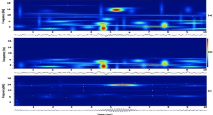
fre-Figure 4: Separation of k-complex and sleep spindle from sleep EEG signal; (a) original signal, (b) the extracted k-complex, (c) the ex-tracted sleep spindle

quency domain corresponds to k-complexes. In Figure 2, each Gabor function is fitted with both wanted and un-wanted components. However, in Figure 3, only desired

370

components are matched. Figures 2(c) and 3(c) share the occurrences of two spindles within the same 10s segment. Nevertheless, according to the chart scale, sleep spindle in Figure 3(c) has higher amplitude compared to those of 2(c). By plotting both original signal and the extracted

375

signal using SSA, it is observed that the separated waves are located in exactly the same positions as their actual places in the original signals. It means that instead of vi-sual analysis, it is possible to automatically localise the waveforms in time domain. Another significant usage of

380

this method is that further to its separating characteristic, it acts as a filter for preprocessing of the signals. Then, the T-F energy map clearly represents each wave by its specific frequency band.

3.2.1. Feature Detection Experiment

385

For this experiment an 8 second, N=2048 sample of the real data which shows the transition of two sleep fea-tures: sleep spindle and k-complex, is selected. Employing the previously discussed procedure for detection of these two features in Constrained SSA section, the sleep spindles

390

and k-complexes can be well separated from EEG signal. Figure 4(a–c) illustrates how constrained SSA can be uti-lized to separate signal into different components simulta-neously.

In order to better illustrate the performance of the

algo-395

rithm, the T-F map of energy of the original signal and the extracted components are represented in Figure 5(a–c).

3.3. Classification of Awake/N1+REM/N2/SWS

The single-channel EEG signals from half of the data were utilized to train the classifier. The rest of the data

400

were utilized to test the reconstructed model. Table 1 illus-trates the statistical description of the training and testing data by 30 second EEG epochs. Most of automatic sleep stage classification methods are employed by different PSG recordings such as EEG, EOG, and EMG [10]. However,

405

in the current work we classified four sleep stages based on

Figure 5: T-F representation of EEG signals of Figure 4; (a) original signal, (b) the extracted k-complex, (c) the extracted sleep spindle

.

Table 1: Information of the training and testing groups Training (Epochs) Testing (Epochs) Awake 196 200 N1+REM 723 804 N2 912 1017 N3 569 579 Total Epochs 2400 2600

single channel EEG signal.

Since N1 and REM have similar characteristics they can be merged into one class. Hence, we attempt to clas-sify four sleep stages consisting of awake, N1 + REM, N2,

410

and SWS. SVM utilized the training data to find the hy-perplane which maximize the margin between the classes. Afterwards, the optimum classification is achieved through applying the separating hyperplane to the testing data.

In order to evaluate the classifier performance,

accu-415

racy, sensitivity, and specificity are calculated. The accu-racy, sensitivity, and specificity are defined as follows:

Accuracy:number of correct decisions total number of cases

Sensitivity:number of true positive decisions number of actually positive cases

420

Specificity:number of true negative decisions number of actually negative cases

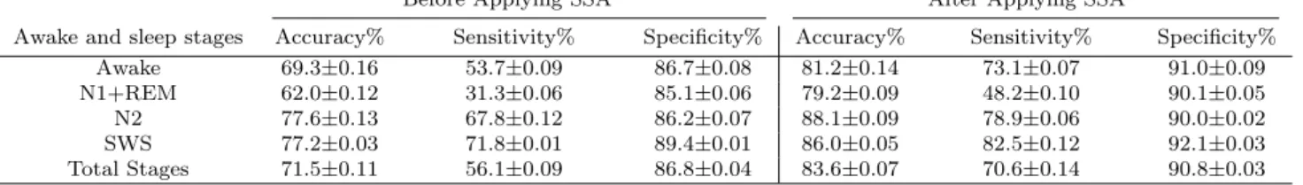
These statistical comparisons are employed over SN data for both before and after preprocessing are shown in Ta-ble 2. From accuracy viewpoint, using SSA, the overall

425

classification performance has been improved. There is in average 12.1% performance improvement in accuracy by applying the proposed method. The significant result achieved here is of immense value since it improves the au-tomatic sleep stage classification to a large extent. When

430

it comes to sensitivity, it is incremented by 14.5% in aver-age for all the staver-ages from before to after preprocessing.

Following the same strategy, four sleep stages are clas-sified for SE and SD nights . The result for SE before and after SSA preprocessing are brought in Table 3. The same

(8)

Table 2: SVM classification results for sleep normal (SN) data before and after applying SSA Before Applying SSA After Applying SSA

Awake and sleep stages Accuracy% Sensitivity% Specificity% Accuracy% Sensitivity% Specificity% Awake 69.3±0.16 53.7±0.09 86.7±0.08 81.2±0.14 73.1±0.07 91.0±0.09 N1+REM 62.0±0.12 31.3±0.06 85.1±0.06 79.2±0.09 48.2±0.10 90.1±0.05 N2 77.6±0.13 67.8±0.12 86.2±0.07 88.1±0.09 78.9±0.06 90.0±0.02 SWS 77.2±0.03 71.8±0.01 89.4±0.01 86.0±0.05 82.5±0.12 92.1±0.03 Total Stages 71.5±0.11 56.1±0.09 86.8±0.04 83.6±0.07 70.6±0.14 90.8±0.03

Table 3: SVM classification results for sleep extension (SE) data before and after applying SSA Before Applying SSA After Applying SSA

Table 4: SVM classification results for sleep deprivation (SD) data before and after applying SSA Before Applying SSA After Applying SSA

Figure 6: Representative four sleep stage classification of 500 epochs acquired using clinical expert (top) and SSA (bottom).

results for SD can be seen in Table 4. Regarding SE, the accuracy for total stages hits the peak of 79.8 ±0.08% after preprocessing compared with 73.0 ±0.10% before that. Similar result can be seen regarding SD with per-formance improvement in sensitivity from 61.4±0.09% to

440

72.1±0.07% using the proposed method. In summary, The accuracy of all sleep stages for 3 types of sleep shows a significant improvement except stage N1+REM, see ta-bles 2–4. We consider S1 and REM as a single stage due to their similarity in EEG pattern. Despite that, the

de-445

tection of N1+REM has not significant changes amongst sleep stages. Since N1 is a transition stage between

wake-fulness and asleep, it is still a challenging issue to find an appropriate feature that would separate N1 from N2 and wakefulness.

450

The k-fold cross validation (CV) technique is used to validate the classifier. The classifier performance shows 11.09 % error though 10-fold CV method. As another ex-ample to shows the efficiency of our proposed method, Fig-ure 6 represents both clinical expert and automatic sleep

455

stage classificationfor 500 epochs 30 seconds long. 3.4. Classification of SE/SN/SD

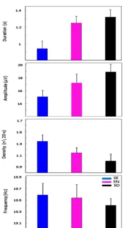
For all the sleep types, it is desirable to compute differ-ent spindle characteristics such as spindle mean amplitude, density, frequency, and lastly the duration. Figure 7

de-460

picts the mean and the standard error of the mean (SEM) for all subjects. The substantial point here is that SN’s values for the duration, amplitude, density, and frequency always fall into a domain limited to the SE nights on one hand as well as the SD nights on the other for all four cases.

465

The mean spindle amplitude and duration are 17.20 (s.d. = 1.1) and 1.25 (s.d. = 0.08) during SN which increase to 18.90 (s.d. = 0.99) and 1.32 (s.d. = 0.08) during SD respectively. Despite this increase, SE’s mean amplitude and duration values significantly reduce to 15.07 (s.d. =

470

0.89) as well as 0.94 (s.d. = 0.09) compared to SN. With regard to the density as well as the frequency, SE’s mean values increase to 1.34 (s.d. = 0.09) and 13.59 (s.d. = 0.2) respectively. SD nights however, diminish to 1.05 (s.d. = 0.1) and 13.41 (s.d. = 0.1) for each aforementioned

param-475

(9)

SE on the characteristics of spindles is novel to our best knowledge so far.

These results not only confirm but also further expand that the characteristics of sleep spindle are remarkably

in-480

fluenced by homeostatic sleep pressure. Our findings in terms of SD validate the reduction of spindle density after SD [24, 25]. Previous works believed that the only sig-nificant change occurs with the density [24, 37]. While, our results prove that the duration, amplitude and

fre-485

quency also change noticeably for SD nights compared to SN nights. Similar to ours, the work in [25] confirms that all the values change for SD and state that the changes are negligible for the duration. Our work, however, steps fur-ther by proving that a significant difference is also exist for

490

duration. This stems from the fact that what is detected with our approach for the automatic detection of the sleep spindles is not subject to any change of scale.

The growth observed in the spindle amplitude of SD case as well as the reduction seen in the frequency

advo-495

cate the hypothesis of a greater level of synchronization in TC when homeostatic sleep pressure is enhanced [25]. Furthermore our findings further stress that with SE, the spindle amplitude goes down whereas the frequency rises. In view of this result, we argue that it is likely that there

500

is a lower level of synchronisation in TC when homeostatic sleep pressure is low.

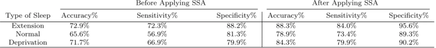
At the next stage, the previously mentioned values cal-culated for different spindle parameters act as the input features for the SVM classifier to categorise sleep types

505

such as SE, SN, and SD. The associated accuracy, sensi-tivity and specificity are shown in Table 5.

4. Conclusions

In this article we incorporated the MP-based T-F rep-resentation of sleep EEG together with an effective

ap-510

proach for refining the data. The refining procedure is based on a known method namely SSA. SSA not only pro-vides all the necessary features of the data for the classifi-cation of sleep stages, but also removes the undesired com-ponents to considerably improve the classification

perfor-515

mance. In addition, thanks to the SSA, parameterising the sleep spindles of SN, SD, and SE has noticeably enhanced to an extent that the sleep types were classified. The pro-posed constrained SSA decomposes the signals into their constituent components in a supervised manner in order

520

to ensure that the desired components are well preserved while the undesired ones are set aside. The proposed hy-brid method paves the way for further analysis of sleep EEG to enable characterisation of sleep abnormalities and many mental and physical disorders. This work has the

525

potential for more diverse set of subjects and features for classifying other set of sleep stages. In addition, here, only normal subjects are involved. Further studies will include those with sleep disorders and other related abnormalities.

530

Figure 7: Mean duration, amplitude, density (number of sleep spin-dles per 20-s epoch), and frequency of sleep spinspin-dles during SE, SN, and SD. Error bars shows the standard error of mean (mean SEM)

.

5. ACKNOWLEDGMENT

The authors wish to thank Prof. Derk-Jan Dijk and Dr. Emma Arbon from the Surrey Sleep Research Cen-tre, University of Surrey, Guildford, UK, for providing the sleep EEG data.

535

References

[1] K. Susmakova, Human sleep and sleepEEG, Journal of Insti-tute of Measurements Science SAS, Slovak Academy of Sciences 4 (2) (2004) 59–74.

[2] J. M. Kortelainen, M. O. Mendez, A. M. Bianchi, M. Matteucci,

540

S. Cerutti, Sleep staging based on signals acquired through bed sensor, IEEE Transactions on Information Technology in Biomedicine 14 (3) (2010) 776–785.

[3] A. Rechtschaffen, A. Kales, A manual of standardized termi-nology, techniques and scoring system for sleep stages of human

545

subjects, US Department of Health, Education and Welfare, Public Health Service, National Institutes of Health, National Institute of Neurological Diseases and Blindness, Neurological Information Network, 1968.

[4] C. Iber, The AASM manual for the scoring of sleep and

asso-550

ciated events: rules, terminology and technical specifications, American Academy of Sleep Medicine, 2007.

[5] J. W. Shephard, Atlas of sleep medicine, Futura Publishing Compony, 1991.

[6] S. Sanei, Adaptive processing of brain signals, John Wiley &

555

(10)

Table 5: SVM classification results for SE, SN, and SD via SSA.

Before Applying SSA After Applying SSA

Type of Sleep Accuracy% Sensitivity% Specificity% Accuracy% Sensitivity% Specificity% Extension 72.9% 72.3% 88.2% 88.3% 84.0% 95.6%

Normal 65.6% 56.9% 81.3% 78.9% 73.4% 89.3% Deprivation 71.7% 66.9% 79.9% 84.3% 79.9% 90.2%

[7] M. K. C. Hublin, M. Partinen, J. Kaprio, Sleep and mortality: a population-based 22-year follow-up study, Sleep 30 (10) (2007) 1245.

[8] N. A. Collop, Scoring variability between polysomnography

560

technologists in different sleep laboratories, Sleep medicine 3 (1) (2002) 43–47.

[9] S. Enshaeifar, S. Kouchaki, C. C. Took, S. Sanei, Quater-nion singular spectrum analysis of electroencephalogram with application in sleep analysis, IEEE Transactions on Neural

565

Systems and Rehabilitation Engineering 24 (1) (2016) 57–67. doi:10.1109/TNSRE.2015.2465177.

[10] J. Virkkala, J. Hasan, A. V¨arri, S. Himanen, K. M¨uller, Au-tomatic sleep stage classification using two-channel electro-oculography, Journal of neuroscience methods 166 (1) (2007)

570

109–115.

[11] C. Berthomier, X. Drouot, M. Herman-Sto¨ıca, P. Berthomier, J. Prado, D. Bokar-Thire, O. Benoit, J. Mattout, M. d’Ortho, Automatic analysis of single-channel sleepEEG: validation in healthy individuals, Sleep 30 (11) (2007) 1587.

575

[12] L. Fraiwan, K. Lweesy, N. Khasawneh, H. Wenz, H. Dickhaus, Automated sleep stage identification system based on time– frequency analysis of a singleEEG channel and random for-est classifier, Computer methods and programs in biomedicine 108 (1) (2012) 10–19.

580

[13] J. ˙Zygierewicz, K. J. Blinowska, P. J. Durka, W. S. S. Niem-cewicz, W. Androsiuk, High resolution study of sleep spindles, Clinical Neurophysiology 110 (12) (1999) 2136–2147.

[14] M. S. Kim, Y. C. Cho, B. Abibullaev, H. D. Seo, Analysis of brain function and classification of sleep stageEEG using

585

daubechies wavelet, Sens. Mater 20 (1) (2008) 1–15.

[15] E. Oropesa, H. L. Cycon, M. Jobert, Sleep stage classification using wavelet transform and neural network, International Com-puter Science Institute, 1999.

[16] U. Malinowska, P. J. Durka, K. J. Blinowska, W. Szelenberger,

590

A. Wakarow, Micro- and macrostructure of sleepEEG, IEEE Engineering in Medicine and Biology Magazine 25 (4) (2006) 26–31.

[17] N. Golyandina, V. Nekrutkin, A. Zhigljavsky, Analysis of time series structure: SSA and related techniques, CRC Press, 2010.

595

[18] S. Sanei, H. Hassani, Singular spectrum analysis of biomedical signals, CRC Press, 2015.

[19] F. Ghaderi, H. R. Mohseni, S. Sanei, Localizing heart sounds in respiratory signals using singular spectrum analysis, IEEE Transactions on Biomedical Engineering 58 (12) (2011) 3360–

600

3367.

[20] S. Sanei, T. Lee, V. Abolghasemi, A new adaptive line en-hancer based on singular spectrum analysis, IEEE Transactions on Biomedical Engineering 59 (2) (2012) 428–434.

[21] D. Jarchi, C. Wong, T. B. a. A. G. R. Kwasnicki, H. Mark and,

605

G. Yang, Gait parameter estimation from a miniaturized ear-worn sensor using singular spectrum analysis and longest com-mon subsequence, IEEE Transactions on Biomedical Engineer-ing 61 (4) (2014) 1261–1273.

[22] S. Kouchaki, S. Sanei, E. Arbon, D.-J. Dijk, Tensor based

singu-610

lar spectrum analysis for automatic scoring of sleep eeg, IEEE Transactions on Neural Systems and Rehabilitation Engineer-ing, 23 (1) (2015) 1–9.

[23] N. Ward, S. M. Cowie, Rosen, V. Roldao, M. D. Villa, T. Mc-Donagh, A. Simonds, M. Morrell, Utility of overnight pulse

615

oximetry and heart rate variability analysis to screen for sleep-disordered breathing in chronic heart failure, Thorax 67 (11)

(2012) 1000–1005.

[24] D.-J. Dijk, B. Hayes, C. A. Czeisler, Dynamics of electroen-cephalographic sleep spindles and slow wave activity in men:

620

effect of sleep deprivation, Brain Research 626 (12) (1993) 190 – 199.

[25] V. Knoblauch, W. L. J. Martens, A. Wirz-Justice, C. Ca-jochen, Human sleep spindle characteristics after sleep depri-vation, Clinical Neurophysiology 114 (12) (2003) 2258 –67.

625

[26] S. G. Mallat, Z. Zhang, Matching pursuits with time-frequency dictionaries, IEEE Transactions on Signal Processing 41 (12) (1993) 3397–15.

[27] S. Sanei, M. Ghodsi, H. Hassani, An adaptive singular spectrum analysis approach to murmur detection from heart sounds,

El-630

sevier Journal of Medical Engineering and Physics 33 (3) (2011) 362 – 367.

[28] J. Mamou, E. J. Feleppa, Singular spectrum analysis applied to ultrasonic detection and imaging of brachytherapy seeds, Jour-nal of the Acoustical Society of America 121 (3) (2007) 1790–

635

1801.

[29] S. Enshaeifar, S. Sanei, C. C. Took, An eigen-based approach for complex-valued forecasting, in: Acoustics, Speech and Signal Processing (ICASSP), 2014 IEEE International Conference on, IEEE, 2014, pp. 6014–6018.

640

[30] R. Vautard, P. Yiou, M. Ghil, Singular-spectrum analysis: A toolkit for short, noisy chaotic signals, Elsevier Journal of Phys-ica D: Nonlinear Phenomena 58 (1) (1992) 95–126.

[31] Y. Tao, E. C. M. Lam, Y. Y. Tang, Feature extraction using wavelet and fractal, Elsevier Journal of Pattern Recognition

645

Letters 22 (3) (2001) 271–287.

[32] F. Ebrahimi, a. E. E. M. Mikaeili, H. Nazeran, Automatic sleep stage classification based on EEGsignals by using neu-ral networks and wavelet packet coefficients, in: Engineering in Medicine and Biology Society, 2008. EMBS 2008. 30th Annual

650

International Conference of the IEEE, 2008, pp. 1151–1154. [33] F. Lotte, M. Congedo, A. Lcuyer, F. Lamarche, B. Arnaldi,

A review of classification algorithms for EEG-based brain– computer interfaces, Journal of neural engineering 4 (2) (2007) R1.

655

[34] G. Zhu, Y. Li, P. P. Wen, in: F. Zanzotto, S. Tsumoto, N. Taat-gen, Y. Yao (Eds.), Brain Informatics, Vol. 7670 of Lecture Notes in Computer Science, 2012.

[35] M. Adnane, Z. Jiang, Z. Yan, Sleep–wake stages classification and sleep efficiency estimation using single-lead

electrocardio-660

gram, Elsevier Journal of Expert Systems with Applications 39 (1) (2012) 1401–13.

[36] V. Vapnik, Statistical learning theory, Vol. 1, Wile, NY, 1998. [37] L. D. Gennaro, M. Ferrara, M. Bertini, Effect of slow-wave

sleep deprivation on topographical distribution of spindles,

Be-665