Speed Up Statistical Spam Filter by Approximation
Zhenyu Zhong,
Member, IEEE,
Kang Li,
Member, IEEE
Abstract—
Statistical-based Bayesian filters have become a popular and important defense against spam. However, despite their effective-ness, their greater processing overhead can prevent them from scaling well for enterprise level mail servers. For example, the dictionary lookups that are characteristic of this approach are limited by the memory access rate, therefore relatively insensitive to increases in CPU speed. We conduct a comprehensive study to address this scaling issue by proposing a series of acceleration techniques that speed up Bayesian filters based on approximate classifications. The core approximation technique uses hash-based lookup and lossy encoding. Lookup approximation is based on the popular Bloom filter data structure with an extension to support value retrieval. Lossy encoding is used to further compress the data structure. While these approximation methods introduce additional errors to a strict Bayesian approach, we show how the errors can be both minimized and biased toward a false negative classification. We demonstrate a 6x speedup over two well-known spam filters (bogofilter and qsf) while achieving an identical false positive rate and similar false negative rate to the original filters.
Index Terms—C.4[Computer Systems Organization]: Performance attributes; H.4[Information Systems Applications]:Miscellaneous; SPAM, Bloom Filter, Approximation
I. INTRODUCTION
I
N recent years, statistical-based Bayesian filters [13], [21], [23], which calculate the probability of a message being spam based on its contents, have found wide acceptance in tools used to block spam. These filters can be continually trained on updated corpora of spam and ham (good email), resulting in robust, adaptive, and highly accurate systems.Bayesian filters usually perform a dictionary lookup on each individual token and summarize the result in order to arrive at a decision. It is not unusual to accumulate over 100,000 tokens in a dictionary, depending on how training is handled [23]. Unfortunately, the performance of these dictionary lookups is limited by the memory access rate, therefore relatively insensitive to increases in CPU speed. As a result of this lookup overhead, classification can be relatively slow. Bogofil-ter [23], a well-known, aggressively optimized Bayesian filBogofil-ter, processes email at a rate of 4Mb/sec on our reference machine. According to a previous survey on spam filter performance [15], most well-known spam filters, such as SpamAssassin [27], can only process at about 100Kb/Sec. This speed might Zhenyu Zhong is with McAfee Research. 4501 North Point Pkwy Ste 300, Alpharetta, GA 30022. Email:edward [email protected]
Kang Li is with the Computer Science department at the University of Georgia, Athens, GA 30602. Email: [email protected]
A shorter version of this paper appeared in the proceedings of the Inter-national Conference on Measurement and Modeling of Computer Systems (SIGMETRICS/Performance 2006) June 2006, Saint-Malo, France
This work was partially supported by NSF grants CNS-0716357 and GRA.GP07.I.
work well for personal use, but it is clearly a bottleneck for enterprise-level message classification.
The goal of our work is to speed up spam filters while keeping high classification accuracy. Our overall acceleration comes from three improvements: 1) Approximate pruning, which reduces the latency of duplicate token search by approx-imating membership checking with Bloom filter. 2) Approx-imate lookup, which allows us to replace memory intensive dictionary lookup with extended Bloom filter based value retrieval. 3) Approximate scoring, which replaces intensive floating point, logarithm operations with lookups on small cache-resident table.
In particular, the major gain of the speedup comes from
“Approximate lookup”, which is enabled by two novel tech-niques. The first techniqueapproximates the dictionary lookup with hash-based Bloom filter [3] lookup, which trades off memory accesses for increase in computation. Bloom filters have recently been used in computer network technologies ranging from web caching [11], IP traceback [28], to high speed packet classifications [5]. While Bloom filters are good for storing binary set membership information, statistical-based spam filters need to support value retrieving. To address this limitation, we extend Bloom filters to allow value retrieval and explore its impact on filter accuracy and throughput. Our second approximation method useslossy encoding, which applies lossy compression to the statistical data by limiting the number of bits used to represent them. The goal is to increase the storage capacity of the Bloom filter and control its misclassification rate.
Both approximations by Bloom filter and lossy encoding introduce a risk of increasing the filter’s classification error. We investigate the tradeoff between accuracy and speed, and present design choices that minimize message misclas-sification. Furthermore, we propose methods to ensure that misclassifications, if they do occur, are biased towards false negatives rather than false positives, as users tend to have much less tolerance to false positives.
Based on the overall approximation on three improvements we mentioned before, this paper presents analytical and ex-perimental evaluations of the filters using these approximation techniques, collectively, known as Hash-based Approximate Inference (HAI). The HAI filter implementations can be applied to most Bayesian spam filters.
Standard metrics are used to measure filter accuracy. A ham that is misclassified as spam is termed as a false positive. The ratio of the number false positives to the total number of actual ham emails is called false positive rate. The false negative rate is analogously defined.
In this paper, the improved filters based on bogofilter [23] or qsf [30] have shown a factor of 6x speedup with similar false negative rates (7% more spam) and identical false positive
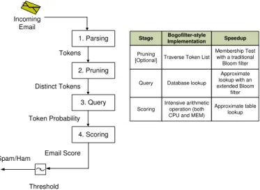
Token Probability Distinct Tokens Tokens Incoming Email 1. Parsing 2. Pruning 3. Query 4. Scoring Threshold Spam/Ham Email Score
Stage Bogofilter-style
Implementation Speedup Pruning
[Optional] Traverse Token List
Membership Test with a traditional
Bloom filter
Query Database lookup
Approximate lookup with an extended Bloom filter Scoring Intensive arithmetic operation (both CPU and MEM)
Approximate table lookup
Fig. 1. Bayesian Filter Stages: The stage with its output is on the left, the speedup techniques corresponding to the stages are on the right.
rates compared to the original filters.
The scope of this paper is limited to optimizing the pro-cessing speed of a particular anti-spam filter and preserving its current classification accuracy. Difficulties and limitations [20], [29] with the general statistic-based anti-spam approach are beyond the scope of this paper.
The rest of the paper is organized as follows: Section II reviews a normal Bayesian filter. Section III reviews the concept of hash-based lookup using Bloom filters and de-scribes the architecture of the HAI filters. Section IV presents our experimental evaluation results of HAI filters. The paper ends with related work and concluding remarks in Section V and VI, respectively.
II. REVIEW OFBAYESIANFILTERS
Here we give a simple review to provide necessary back-ground for the discussion of the filter acceleration.
A. Anatomy of Bayesian Filters
Bayesian probability combination has been widely used in various message classifications. To classify a message, a traditional Bayesian filter typically processes the message in 4 stages as shown in Figure 1: 1) Parsing stage, where the message is parsed into a set of tokens (words or phrases). 2)
Pruning stage, where the distinct tokens are extracted from the parsed result. Pruning is an optional stage of Bayesian filters depending on whether the score calculation considers duplicated tokens or not.1 3)Query stage, which looks up for each token’s occurrences in previously known types (spam or ham). The frequency statistics information is obtained from a set of training messages which are labeled explicitly as spam or ham and stored in a database for future lookup. 4) Scoring stage, where Bayesian filters combine all the token statistics of an incoming message to an overall score by a Bayesian probability calculation [14]. Finally, filtering decision is made based on the score and a pre-defined threshold.
1We investigate several Bayesian filters implementations and find that some
implementations have pruning stage for example, bogofilter, spamAssassin while others such as qsf, spamBayes don’t.
Stage 1. Training
Parse each email into its constituent tokens Generate a probability for each token W
S[W] =Cspam(W)/(Cham(W) +Cspam(W))
store spamminess values to a database Stage 2. Filtering
For each message M
while (M not end) do
scan message for the next tokenTi
optional token pruning
query the database for spamminess S(Ti)
calculate accumulated message probabilities
S[M] andH[M]
Calculate the overall message filtering indication by:
I[M] =f(S[M], H[M]) f is a filter dependent function, such asI[M] = 1+S[M]2−H[M]
if I[M]> threshold
msg is marked asspam
else
msg is marked asnon-spam
Fig. 2. Outline for A Bayesian Filter Algorithm
B. Score Calculation in Naive Bayesian filter
Most previous studies on statistical filters focus on various types of Bayesian probability calculation [14]. Usually, these filters first go through a training stage that gathers statistics of each token. The statistic in which we are mostly interested for a tokenT is its spamminess, calculated as follows:
S[T] = Cspam(T)
Cspam(T) +Cham(T)
(1) where Cspam(T) and Cham(T) are the number of spam or ham messages containing tokenT, respectively.
To calculate the possibility for a message M with tokens
{T1, ..., TN}, one needs to combine the individual token’s
spamminess to evaluate the overall message spamminess. A simple way to make classifications is to calculate the product of individual token’s spamminess (S[M] = QN
i=1S[Ti]) and
compare it with the product of individual token’s hamminess (H[M] =QN
i=1(1−S[Ti])). The message is considered spam
if the overall spamminess product S[M] is larger than the
hamminess productH[M]. S[M] =C−1(−2 ln( n Y i=1 S[Ti]),2n) (2) H[M] =C−1(−2 ln( n Y i=1 (1−S[Ti])),2n) (3)
The above description is used to illustrate the idea of statistic based filters using Bayesian classifications. In practice, various techniques are developed for combining token proba-bilities to enhance the filtering accuracy. For example, many
0 1 0 1 1 H1 H2 TOKEN H3 Hash Functions (m bits) Bit Vector
Fig. 3. Training for a Bloom Filter
Bayesian filters, including bogofilter and qsf, use a method suggested by Robinson [25]: Chi-squared probability testing. The Chi-squared test calculatesS[M]andH[M]based on the distribution of all the tokens’ spamminess ({S[T0], S[T1], ...})
against a hypothesis, and scalesS[M]andH[M]to a range of 0 to 1 by using an inversed chi-square function. Here we give the equations 2 and 3 to calculate S[M] and H[M], where
C−1()is the inversed chi-square function,2nis the degree of
freedom and nis the number of distinct tokens in the email. Details of this algorithm are described in [23], [25].
To avoid making filtering decisions whenH[M]andS[M]
are very close, several spam filters [21], [23], [30] calculate the following indicator instead of comparing H[M] and S[M] directly
I[M] = 1 +S[M]−H[M]
2 (4)
When I >0.5, it indicates the corresponding message has a higher spam probability than ham probability, and should be classified accordingly. In practice, the final filter result is based onI > thresh, wherethreshis a user selected threshold. For conservative filtering,threshis a value closer to 1, which will filter fewer spam messages, but less likely to result in false positives. As thresh gets smaller, the filter becomes more aggressive, blocking more spam messages but also at a higher risk of false positives. A general Bayesian filter algorithm is presented in Figure 2. It is first trained with known spam and ham to gather token statistics and then classifies messages by looking at its token’s previously collected statistics. A more detailed description of the Bayesian spam filter algorithm can be found in several recent publications [13], [21], [23].
III. OURAPPROACH
A. HAI Filter Architecture Overview
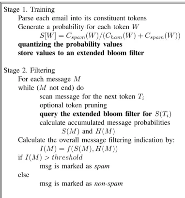
This section presents Hash-based Approximate Inference (HAI) filter. The HAI algorithm is presented in Figure 4, which applies a combination of 3 speedup techniques including
approximate pruning, approximate lookup and approximate
Stage 1. Training
Parse each email into its constituent tokens Generate a probability for each token W
S[W] =Cspam(W)/(Cham(W) +Cspam(W)) quantizing the probability values
store values to an extended bloom filter
Stage 2. Filtering
For each message M
while (M not end) do
scan message for the next tokenTi
optional token pruning
query the extended bloom filter for S(Ti)
calculate accumulated message probabilities
S(M)andH(M)
Calculate the overall message filtering indication by:
I(M) =f(S(M), H(M))
if I(M)> threshold
msg is marked asspam
else
msg is marked asnon-spam
Fig. 4. HAI Filter Algorithm (Highlights are changes made to Bayesian filters)
scoringcorresponding to the typical Bayesian filters as shown in Figure 1.
In thePruning stage, the conventional Bayesian filters such as bogofilter, conduct duplicate token search by traversing a to-ken list. HAI filter replaces it with a fast membership checking on a compact traditional Bloom filter (see section III-B). The Bloom filter is initialized to be empty and each newly parsed token from the message is first checked against the Bloom filter. The token is discarded if it is already a member of the set; otherwise it becomes a member of the set and is passed onto the query stage. The effectiveness of this approximation is presented in section IV-H.
In theQuery stage, Bayesian filters often rely on databases such as BerkeleyDB to store the token statistics. However, the multiple memory access latencies limit the database lookup speed. Analytically, this limitation shows the advantage of using HAI over traditional database index structure.
• HAI lookup: The number of memory accesses per lookup depends only on the number of hash functions. Thus the complexity isO(h)on memory accesses where
his a small constant number. The use of the hash func-tions is discussed in detail in the following subsecfunc-tions.
• Database lookup: Traditional lookup using Database such as BerkeleyDB, which employs the BTree in-dex structure, usually requiresO(logdT /2e(N)) compar-isons(potential memory accesses), where N is the total number of the records andT is the order of the tree.
• Small memory footprint: Besides the reduction of the total number of memory accesses, the small memory footprint of a Bloomfilter allows us to take the advantage of memory cache for further speedup.
x x 1 1 x 0 0 H1 H2 TOKEN H3 Hash Functions AND bit−wise Query Output Bit Vector 1: in−set; 0: not−in−set (m bits)
Fig. 5. Query a Normal Bloom Filter
Accordingly, we approximate the token statistics lookup into an extended Bloom filter with value retrieval support (see section III-C). Specifically, the approximation in this stage includes approximate quantization and approximate lookup (see section III-D). The accuracy of HAI filter relies on the setup of the extended Bloom filter. The details of controlling the accuracy of query stage are discussed in section III-E.
In theScoring stage, the overall email score is usually calcu-lated by combining all the token probabilities via an inversed chi-square function (Fisher method [25]). It takes intensive floating point, logarithm operations if precise calculation is used. HAI reduces this overhead by replacing it with a two dimensional cache-resident percentage points of chi-square distribution table. This table can be pre-calculated based on the inputs stated in equations 2 and 3. The effectiveness of this approximation is presented in section IV-H.
B. Bloom Filters
A Bloom filter is a compact data structure designed to store query-able set membership information [3]. Bloom filters were originally invented by Burton H. Bloom to store large amounts of static data such as English hyphenation rules.
A Bloom filter consists of a bit vector of length m that represents the set membership information about a dictionary of tokens. The filter is first populated with each member (token) of the set (Figure 3 shows a Bloom filter in this training phase). At the training phase, for each token in the membership set, h hash functions are computed on the token producing h
hash values each ranging from 1 to m. Each of these hash values addresses a single bit in the m-bit vector, and sets that bit to 1. Hence for perfect hashes, each token causes h bits of the m-bit vector to be set to 1. In the case that a bit has already been set to 1 because of hash conflicts, that bit is not changed.
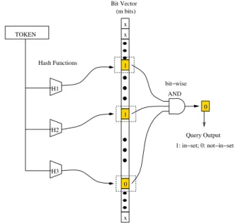
Querying a token’s membership is similar to the training process. Figure 5 shows a Bloom filter in the query stage with
a non-member token. For a given token, h hash results are produced and each addresses one bit. The token is guaranteed not in the set if any of these bits is not set to 1. If all thehbits are set to 1, the token is said to belong to the set. This claim is not always true because the fact of thesehbits being 1 could be a result of the hashes of multiple other member tokens. This case is considered to be a false positive for membership testing. The likelihood of false positive occurrence can be made very small by carefully choosing the size of bit vector and number of hash functions. We illustrate this with a brief overview of the false positive probability derivation: Assuming perfect hash functions and a m-bit vector, the probability of setting a random bit to 1 by one hash is 1/m, and thus the probability that a bit is not set by a single hash function is
(1−1/m). Forhhash functions, the probability that a bit is not set by any of the hashes is(1−1/m)h. For a member set
withntokens, the probability of a bit not set is
P0= (1− 1 m)
n∗h (5)
and the probability of a bit set to 1 is
P1= 1−(1− 1 m)
n∗h
(6) For a non-member token to be misclassified as a possible set member, all thehbits addressed byhhash functions must be 1. Thus the probability of a false positive is
Pm,n,h(fpos) = (1−(1− 1 m)
n∗h)h (7)
Note that the above probability is the false positive for token membership testing, which is very different from the false positive of email message classification.The latter usually combines multiple tokens’ spamminess values in order to arrive at a probability result. The next section discusses how to control the effect of the Bloom filter misclassification to minimize the email message misclassifications.
C. Extending Bloom Filter
Traditional Bloom filters only make membership queries that verify whether a given token is in a set, but applications such as spam filters must retrieve each token’s associated probability value. We extend the Bloom filter to serve for value queries while preserving Bloom filter’s desired original operating characteristics. For a given token in the member set, the extension returns a value that corresponds to a given token. The idea of this extension is to simply maintain a two-dimensional vector, which has a total bit-vector size of m
bits, and every hash output points to one of the r entries, each of which has q bits (i.e m is the product of r and q). The traditional Bloom filter becomes a special case of this extension that uses one bit per entry (q=1).
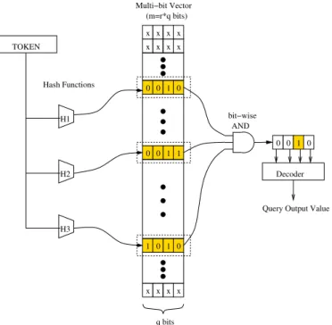
Figure 6 shows the structure of this Bloom filter extension. It works in the following way to support value retrieval. During the Bloom filter training phase, each training token runs through the hash functions and addresseshentries (each entry contains q bits). Assume the token has an associated value (in integer)v in a range of 0 to q−1. The valuev is
x x x x x x x x x x x x 0 0 1 0 1 0 1 0 1 0 0 1 0 0 1 0 q bits H1 H2 TOKEN H3 Hash Functions AND bit−wise
Query Output Value Decoder Multi−bit Vector
(m=r*q bits)
Fig. 6. Bloom Filter Extension for Value Retrieving Query (The Bit-Vector hasrentries and q bits per entry)
then stored to the Bloom filter extension by setting the v th-bit to 1 on all these h entries. During the query phase, each incoming token also goes through the hashing and addresses
h entries. The query outcome for this token is based on the logical AND of all hentries. If none of the bits is set in the logical AND output, it indicates that the token in the query is not in the training set. If a bit is set, then based on the position of the bit, we retrieve the value associated with the token.
D. Extended Bloom Filter based Approximate Lookup
The query stage is improved by two means including approximation by quantization and approximate lookup.
1) Approximation by Quantization: To effectively use the Bloom filter extension for approximate value retrieval queries, we introduce lossy encoding (quantization) to represent the individual token’s spamminess value. Consider the way that the Bloom filter extension represents a statistical value by marking one bit of a q-bit entry. It has to adopt some quantization technique if the amount of potential numbers to be represented is infinite.
During the training phase, each token T obtains a proba-bility value pbased on it shows up in ham and spam. HAI differs from traditional Bayesian filter by mapping a token’s probability value p to an integer value v between 0 and
q−1, where q is a parameter of the Bloom filter extension called quantization level. The token is then considered to be associated with value v for storing and retrieving with the Bloom filter extension. When used at the end to calculate a message’s spamminess, a token’s probability value v is approximately mapped back to p based on the quantization mapping.
This paper studies the effect of different quantization levels on Bloom filter’s lookup performance. Two aspects of
quan-tization effects need to be addressed. First, we would like to choose an optimal quantization level (q), which affects both the size (m) of the Bloom filter’s bit-vector and the Bloom filter misclassification rate. The latter is discussed in the next subsection.
Second, for each given quantization level, we would like to pick the optimal mapping between the values to be quantized and the values after quantization for minimal errors. This paper uses Lloyd-Max algorithm to obtain the optimal quantizer for the token spamminess values for each given quantization level. The Lloyd-Max [1] algorithm is borrowed from previous studies of optimal quantization (such as those used in MPEG [12]) in the area of lossy encoding [2]. The Lloyd-Max algorithm is one of the popular algorithms that make a non-uniform optimal quantization that provides minimal “quality distortion” to videos.
2) Approximate Lookup: This extension allows the Bloom filter to support value retrieval queries at a cost of higher error rate compared to the original Bloom filter. Two types of misclassification could happen in this extended Bloom filter. This approximation happens in the query stage of bayesian filter in Figure 1.
First, similar to the original Bloom filter, the extended one could misclassify a non-member token as a member and mistakenly provide a value. The chance of such false positive misclassification increases because if any bit of the multi-bit output entry is set to one by hash conflicts, a false positive will occur. Assuming perfect hashes and uniform distributions of the values to be stored, we derive the theoretical error rate. The details are presented at [31]. Some key results are: The possibility for a single bit being zero in the output is
Pm,n,h(0) = 1−Pm,n,h(fpos) = 1−(1−(1− 1 m)
n∗h)h
(8) With the final logical AND output having q bits, the possibility of false positive becomes
Pm,n,h,q(fpos) = 1−(Pm,n,h(0))q (9)
Second, a new type of error occurs when more than one bit of the final Bloom filter outcome are set to 1. The probability of a multi-bit marking is equivalent to one minus the probability of all bits being set to zero and the probability of only one bit getting 1.
Pm,n,h,q(multi) = 1−(Pm,n,h(0))q
−q∗(1−Pm,n,h(0))∗(Pm,n,h(0))(q−1) (10)
The probability rates for both types of errors depend on the number of tokens (n), the Bloom filter bit-vector size (m), the number of hash functions (h), and the quantization level (q). Figure 7 shows a theoretical error rate for a dictionary with 220,000 tokens versus various bit-vector sizes from 0 to 1 MB, 4 or 8 hash functions, and 4 or 8 bits quantization respectively. The dictionary size is selected based on the rec-ommended token sizes by bogofilter [23]. The results indicate that the selection of Bloom filter parameters (m,h,q) affects the misclassification rate significantly. For a small number of hash functions, the Bloom filter can reach less than a 0.1% token misclassification rate with less than 1MB memory under small quantization levels (4 or 8 bits).
1e-06 1e-05 1e-04 0.001 0.01 0.1 1 0 200 400 600 800 1000
Token Misclassification Prob
Bloom Filter Size (KBytes)
Dictionary=220,000 Tokens; H: Hash; Q: Quantization Bloom, H4 Ext-Bloom, H4,Q4 Extended Filter, H4,Q8 Bloom, H8 Ext-Bloom, H8,Q4 Ext-Bloom, H8,Q8
Fig. 7. Lookup Error Rate vs. Bitmap Sizes
E. Control the Lookup Accuracy
This section discusses how to reduce the total errors caused by the two approximations (quantization and approximate lookup) in order to limit their impact to the final message classification errors. We control the impact of these errors by choosing appropriate Bloom filter size and quantization level that minimize the total lookup errors. In the case of multi-bit marking, we control the query outcome in a way that is biased toward false negative classifications.
1) Selection of Bloom Filter Parameters: The selection of the bloom filter parameters is a complex process. In practice, it is actually based on at least three types of conditions:
theoretical limit on false classification rate, physical hardware constraints, and information to be stored. For example, the hardware contraints such as level-2 cache capacity affect the throughput of the Bloom filter. Moreover, the data to be stored in the Bloom filter also affects the performance especially the accuracy of the lookups. In order to provide comprehensive guide for the use of the Bloom filter, we first provide the theoretical estimation of the lookup accuracy in this section, followed by experimental evaluations in Section IV.
For a given dictionary size (n), to minimize the lookup errors and achieve high-speed lookups requires a careful se-lection of Bloom filter parameters: the size of the Bloom filter (m), the number of hash functions (h), and the quantization level (q). The parameter selection has to balance the error rate and the lookup speed. For example, large Bloom filter size is generally preferred for low misclassification rate, but Bloom filters with a size larger than the cache would degrade the query performance. The parameter selection also has to balance the approximation errors caused by quantization and hash-based lookups. For example, higher quantization levels (more bits used for quantizations) are preferred to store high precision values; but for a fixed Bloom filter size, higher quantization levels cause fewer rows in Bloom filter and thus increase misclassification rate (as indicated by Equation 9 and 10).
Previous Bloom filter applications [4], [5] have extensively studied the selection of Bloom filter size (m) and number of
hash functions (h) involved in the tradeoff between size and error rate. The Bloom filter extension shares similar guidelines regarding the selection of these two parameters (m and h). This section focuses on the selection of quantization level (q) which is unique to this Bloom filter extension.
We define the problem of picking the appropriate quanti-zation level as the following: For a given Bloom filter size m=r∗q, we would like to pick an appropriate quantization level q that minimizes the error between a token’s lookup outcome value and the token’s original statistical value.
The expected error between a lookup outcome and its orig-inal value is a probability combination of the misclassification error (Elookup) and the quantization error (Equantiz). The following equation represents the error as the sum of these errors:
Eoverall=P∗Elookup+ (1−P)∗Equantiz (11)
in which P is the probability of token misclassifications. To make a good choice of the Bloom filter parameters, we would need to know the distribution of the values to be quantized and stored in the Bloom filter. This is available for every training set, and its parameters may be determined experimentally. If the theoretical distribution of token statistics is known, the optimal parameter selection, in particular the appropriate quantization level for a given bit-vector size, can be done through a theoretical analysis.
For example, we assume the values to be stored follow a Gaussian distribution G(α = 0.5, σ), where G(α, σ) repre-sents a Gaussian distribution with a mean of αand variance
σ.
If no Bloom filter misclassification occurs, the value coming out from a Bloom filter lookup is assumed to be the same as original value plus a quantization error. The distribution of this error, Equantiz, follows a Gaussian distribution G(α = 0, σ/(2q)), whereq is the number of quantization levels.
If a Bloom filter misclassification occurs, e.g a token T
that is not seen in the training set was mistakenly given a lookup outcome v, the lookup error is determined by v and the appropriate value for tokenT. We assume that the values of random tokens that are not in the training set should follow a Gaussian distributionG(α= 0.5, σ). This assumption reflects the idea that an unknown token should be considered to be neutral. We further assume that the classification outcome v
is independent to the token when misclassifications occur, and thus v follows G(α= 0.5, σ/(2q)). With these assumptions, the lookup error Elookup follows a Gaussian distribution
G(α= 0, σ+σ/(2q)).
In addition, assuming the lookup misclassification occurs independently from the quantization errors, the linear com-bination of two Gaussian distributions is still a Gaussian distribution. The overall query outcome error thus has a mean
αof 0, and variance is
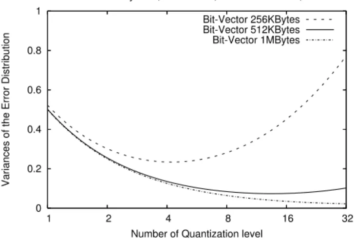
(1−Pm,n,h,q)∗(0.5/q) +Pm,n,h,q∗(σ+σ/(2∗q)) (12)
in which, Pm,n,h,q is the misclassification probability of a Bloom filter that has q levels of quantizations, h hash func-tions, total size m bits, and store values for n tokens. The
0 0.2 0.4 0.6 0.8 1 32 16 8 4 2 1
Variances of the Error Distribution
Number of Quantization level Dictionary=220,000 Tokens; 4 Hash Functions;
Bit-Vector 256KBytes Bit-Vector 512KBytes Bit-Vector 1MBytes
Fig. 8. Error Distribution Variance vs. Quantization Levels
0 0.2 0.4 0.6 0.8 1 32 16 8 4 2 1
Variances of the Error Distribution
Number of Hash Functions
Dictionary=220,000 Tokens; 4 bits Quantization;
Bit-Vector 256KBytes Bit-Vector 512KBytes Bit-Vector 1MBytes
Fig. 9. Error Distribution Variance vs. Number of Hash Functions
best quantization level isqsuch that it minimizes the value of Equation 12.
Figure 8 shows the predicted error variances of the overall lookup error distribution assumingσ= 1. The result indicates that for a dictionary of 220,000 tokens, the quantization levels should be around 4 to achieve a smaller error variances for small bit-vector size (e.g 256Kbytes). Quantization levels smaller than 4 or larger than 6 would have larger error on average. When larger bit-vector is used, quantization levels larger than 4 lead to smaller errors.
Figure 9 shows the predicted error variance for a Bloom filter with the same dictionary size, a fixed quantization level of 4, but with different hash functions. The result matches the intuition that, for a fixed quantization level, the selection of other Bloom filter parameters (h and m) agrees with early studies [4], [5]: for small bit-vector size, the number of hash functions needs to be small (around 6 for the 256Kbytes Bloom filter) in order to achieve a lower misclassification rate. As size of Bloom filter increases, more hash functions can be used to achieve a lower misclassification rate, but the increase in effectiveness is modest.
The above estimation is based on an unrealistic assumption
of value distributions. In real messages, the occurrence of tokens is not independent and identically distributed (iid). This result is only for analytical purpose and is only shown as a guideline for selecting the Bloom filter parameters. The real error rate is determined by the specific distributions and messages. Furthermore, our overall concern is the final message classification performance (false positives, false neg-atives, and throughput). Therefore we used real messages to make a realistic study through experiments in order to evaluate the selection of the Bloom filter parameters. The results are presented in Section IV.
2) Policy for Multi-Bits Errors: The previous subsection discusses the selection of Bloom filter parameters to minimize the possibility of lookup errors. Although very rarely, errors could still occur. When a conflict caused by multiple bits marking occurs, interpreting the outcome based on any bit could cause lookup error which later could potentially cause a message misclassification.
Although this can not be completely avoided, the impact of this error can be further minimized by making error biased toward a false negative classification rather than a false positive. When multiple possible values come out from one lookup query, we chose the smallest value as the Bloom filter outcome so that even if it is wrongly chosen, the error only makes the classification result less likely as spam. We evaluated the effectiveness of this policy and the result is presented in Section IV-G.
3) Selection of Hash Functions: Another fact that can affect Bloom filter lookup speed is the complexity of the hash functions. Popular hash functions, such as MD5 [24], have been designed for cryptographic purposes. However, the effort to prevent information leaking is not the focus of hash-based lookup, whose main concern is the throughput. Therefore, simple but fast hash functions are preferred. This preference of choosing simple hash functions has also been used in [9], [19]. In this paper, we adopt two strategies to design the hash functions. One strategy is to simplify the well-known hash function, such as MD5. The other strategy is to build a fast hash function from scratch. Details of the hash function selection are presented in the evaluation section.
IV. EVALUATION
This section presents our experimental evaluation of HAI filters. First we describe our methodology. Second we show the effect of changing Bloom filter parameters.
A. Methodology
We studied the effectiveness of HAI filters by measuring its throughput and filter accuracy with real messages (24,000 ham messages and 24,000 spam messages) obtained from the Internet. The ham messages are from the ham training set released by SpamAssassin [27] and from several well-known mailing-lists, including end-to-end [8] and perl monger [22]. The spam messages are obtained from SpamArchive [18]. We split the data set into a training set and a test set. Throughout this section, except explicitly specified, we use 10,000 spam messages and 10,000 ham messages as the training set, which
0 500 1000 1500 2000 2500 3000 3500 4000 4500 5000 1.0GHz 1.2GHz 1.4GHz 1.6GHz 1.8GHz
Per Message Time (microseconds)
CPU Speed Bogo:HAI (4.95:1) Bogo:HAI (5.26:1) Bogo:HAI (5.78:1) Bogo:HAI (6.06:1) Bogo:HAI (6.16:1) scoring query pruning parsing
Fig. 10. Filter Process Time Breakdown for Various CPU Speeds (HAI filter: 512KB bit-vector, h=4,q=8; Numbers inside the figure are speedup ratio)
produces a dictionary with 320,976 tokens. The rest of the messages are used for filter testing. The testing sets are further divided into two sets based on their sources. Dataset1 is composed of 10,000 ham from mailing-lists and 10,000 spam from SpamArchive [18]; dataset2 is composed by 4000 ham messages from SpamAssassin [27] and another 4000 spam from SpamArchive.
The experiments are conducted on a PC server with a AMD Athlon64-3000 CPU, 1GB RAM and 512kB Level 2 cache. The CPU speed is scalable by software and by default runs at 1.8GHz. To avoid disk I/O latency, we create ramdisk to store the test set, so that only non-disk I/O are involved for message processing in the experiments.
We built two HAI filters based on well-known Bayesian filters: bogofilter [23] and qsf [30]. Since bogofilter is faster than qsf according to both our measurements and other stud-ies [15], except explicitly specified, all experimental results presented in this section are in the form of a comparison between the bogofilter based HAI (labeled HAI filter) versus the original bogofilter (labeled bogofilter) under the same experiment condition.
B. Overall Performance
This section summarizes the overall HAI performance with well-selected Bloom filter parameters. The results presented in this section are based on a Bloom filter with a total size of 512 Kbytes, 4 hash functions, and an 8-bit quantization. The performance comparison results are in terms of both filter throughput (messages per second) and filter accuracy (both false positives and false negatives). The filter accuracy results presented in this subsection are based on a filter threshold of 0.5. Detailed studies for the selection of this threshold as well as other Bloom filter parameters are presented in the later part of the evaluation section.
Table 1 shows the overall performance of bogofilter, qsf, and their HAI modifications. This result indicates that, for a Bloom filter size at 512KB, HAI filters can handle 2583 messages per second (i.e. 41Mbps for 2KByte size messages). HAI gets
0 1000 2000 3000 4000 5000 1k 2k 4k 8k 16k Throughput (Msgs/sec)
Message size (Bytes) HAI (MD5)
Bogofilter
Fig. 11. Message Size vs Throughput (HAI filter: 512KB, h=4, q=8)
a 6 to 8 times throughput speedup compared to bogofilter and qsf respectively, without introducing any additional false positives. The speedup comes with the penalty of higher false negative rates for HAI filters. Such penalty (e.g. about 7% of overall spam in dataset1) might look significant, but that still corresponds to more than 90% spam messages being blocked by the filter2. Whether this tradeoff is worthy or not completely depends on each particular site’s needs. The goal of this paper is not to advocate high throughput over accuracy but to provide a study of the trade-off between throughput increment and accuracy penalty. Furthermore, multiple levels of spam filtering can be used. For example, HAI filter quickly scanning all incoming messages, and later applying heavy filters only to ”unsure” messages.
C. Detailed Breakdown for Throughput
This section presents an in-depth study on the source of this speedup by looking at the detailed behaviors of bogofilter and HAI filter. We decompose both bogofilter and HAI to four steps (parsing, pruning, queryand scoring) and measure the time spent on each step per message. These 4 steps have been described in the overview of Bayesian filter in section II-A. To reiterate, the parsing step divides the message to tokens based on common delimiters; thequerystep takes each token and uses it as a key for a database lookup to retrieve the corresponding token statistics; and thescoringstep combines all the query outcomes and calculates an overall message spamminess value.
Bogofilter adds apruningstep betweenparsingandquery. Performance-wise, this pruning step is used to reduce the unnecessary lookup. It removes duplicated tokens so that each unique token only triggers one query. It also eliminates tokens that are believed to be useless for anti-spam. Such tokens include email message id, MIME labels etc. They are discarded during the training phase and thus are not in the token database (DB). The pruning step of our HAI filter only
2We investigated the nature of those messages that causes additional false
negatives to HAI. Most of them are non-English messages. It just happens to be the case that more of these spam are selected to Dataset1 than Dataset2.
TABLE I
PERFORMANCECOMPARISON BETWEENBOGOFILTER, QSFANDHAI FILTERS ON APC SERVER WITHAMD ATHLON64 (M=512K,H=4,Q=8,
THRESH=0.5,ANDCPU=1.8GHZ)
BogoFilter HAI (bogo) filter QSF HAI (QSF) filter Throughput (msg/sec) 418 2583 101 871 Dataset1 False Positive 0% 0% 0% 0% Dataset1 False Negative 2.24% 9.36% 3.41% 9.21% Dataset2 False Positive 0.20% 0.20% 0.23% 0.23% Dataset2 False Negative 4.00% 4.80% 6.80% 9.83%
preserves the function of removing duplicated tokens to keep the same scoring method (each token counts only once). It uses a standard (not extended) Bloom filter to check token duplica-tions. This Bloom filter works independently to the extended Bloom filter for the query step. The duplicate token checking initializes a small Bloom filter (2KB in our implementation) to all zeros for each incoming message, and queries and trains the filter at the same time. When a token arrives, it is first tested against the Bloom filter. If the membership testing returns true, the token is considered a duplicate and discarded. Otherwise, the token is put in the Bloom filter as a new member token and will be used in the query step. The detailed algorithm for this duplication checking can be found in our early work on fast packet classification [5].
We measured the processing time for each step by testing bogofilter and HAI with Dataset1. The average message size for Dataset1 is around 2KByte, and each message contains about 180 unique tokens. Figure 10 shows the bogofilter versus HAI processing time comparison per message. It is obvious that query and pruning are the two bottleneck steps of bogofilter, and the speedup of HAI comes from these two steps. HAI gains speedup for the query step by reducing the number of memory accesses for each token lookup. An HAI filter’s lookup requires a small amount of memory accesses that only depends on the number of hash functions and the size of Bloom filter, not the total number of stored tokens as in the database lookup case. In addition, by making the bloom filter size small, most or all of it can fit in cache for lower memory access latency. This effect of cache size is presented in the next subsection. Bogofilter’s query step, on the other hand, operates on Berkeley DB, which is implemented by a Btree. The query requires multiple comparisons between the input token and tokens in the DB and the number of comparisons on average is proportional to the logarithmic of the total tokens in the DB. Although a faster indexing mechanism is possible, a DB lookup essentially has to have a few token comparisons, whereas these comparisons are completely avoided in HAI by the use of the extended Bloom filter.
The HAI also gains significant speedup in its pruning step. We did not include this as part of the general HAI solution for two reasons. First, not all the Bayesian filters avoid searching duplicated tokens as bogofilter does. Second, there is no fundamental reason that a DB-based Bayesian filter can not replace its pruning step with the one used by HAI. Even if bogofilter adopts the same pruning step as HAI, without changing to approximate query as HAI does, bogofilter would still be multiple times slower than HAI to process a message. In addition to the throughput gain against bogofilter, HAI’s
TABLE II
AMD L2 CACHEPERFORMANCECOUNTERS FOR THEQUERYSTEPPER
MESSAGE(CPU=1.8GHZ,AND FORHAIFILTER:H=4,Q=8)
Configuration L2 Miss L2 Hit Query Time HAI (128KB) 8 835 202µs HAI (256KB) 30 1120 208µs HAI (512KB) 51 1264 216µs HAI (1MB) 387 1066 257µs BogoFilter 2157 605 1716µs
throughput scales better as CPU speed increases. The AMD Athlon64 based desktop supports CPU scaling, we adjusted the speed from 1.0 GHz to 1.8GHz and measure the throughput of both filters. Figure 10 shows a comparison of bogofilter and HAI for various CPU speeds. Although both filters take less time to process a message as the CPU speed increases, the speedup ratio for HAI versus bogofilter increases as CPU speed becomes higher.
We also inspect the effect of message size on the speedup ratio. Figure 11 compares the throughput between bogofilter and HAI with different message sizes. The bogofilter stores 44k tokens in its database, while the same number of tokens are stored in our 512kB HAI filter. The result shows that as messages get large, the speed up ratios starts to decrease.The parsing step increases strictly proportional to the message sizes, but the number of unique tokens does not increase in a strict linear fashion. The bottleneck starts to shift from query and pruning toward parsing.
Although message size has impacts on the throughput, even with a jumbo message size, token query continues consuming a significant amount of processing time for bogofilter, and approximate classifications would still improve bogofilter’s performance. Consider that regular emails are often with a small message body except those with attachments, HAI lookup gains benefits on speedup in most of the cases.
D. Effect of Bloom Filter Size
In this subsection we study the effect of Bloom filter size on the filter accuracy and processing throughput. Both the throughput and accuracy measurements were obtained from experiments using the Dataset1.
For the effect of Bloom filter size on throughput, Figure 12 shows that the per message processing times are about the same for the HAI filters with a Bloom filter size less than 512KB. After the bloom filter becomes close to or exceeds L2 cache size (512KB), the processing time in general increases as the Bloom filter size increases towards 16 Megabytes. The AMD Athlon64 processor provides performance counters for
0 50 100 150 200 250 300 350 400 450 500 16M 8M 4M 2M 1M 512K 256K 128K 64K
Per Message Time (microseconds)
Bloom Fitler Size (Bytes) scoring
query pruning parsing
Fig. 12. Processing Time VS. Bloom Sizes (AMD CPU=1.8GHz,h=4,q=8)
specific processor events, such as data cache hits and misses, to support memory system performance monitoring. To confirm the cache size effect, we capture the L2 cache performance counters before and after each query step.
Table 2 contains the average L2 memory access and miss counters of the query step for HAI or bogofilter to process a message. As shown by Table 2, smaller Bloom filters can be put in higher level CPU caches and have fewer cache misses compared to larger Bloom filters. HAI filters clearly have a higher L2 hit rate than bogofilter. L2 cache behavior is not the single factor that determines the processing time; the total computation of a program, memory access pattern, as well as L1 cache behaviors all affect the query time, and a slight adjustment to the program (e.g different Bloom filter sizes) could change these memory accesses behaviors. This is also why the total L2 accesses (hits+misses) changes across different filter setups. Although we can not directly calculate the query time from L2 misses, it is clear that the cache accesses differences is a major source for the query time increment over filter size increment, which is shown in Figure 12.
The gain in throughput comes with a penalty on filter accuracy. To have an overall picture about how much change was brought to the filter accuracy by HAI, we present the false positive and false negative probabilities for the complete range of possible filtering thresholds from 0 to 1. Figure 13 shows a summary of the filter accuracy for HAI filters with various Bloom filter sizes ranging from 64KB to 16MB.
For the false positive result shown on the left half of Figure 13, HAI filters with smaller than 512KB show significant differences compared to those of bogofilter. The smaller the Bloom filter size, the higher differences they can make.
However, for Bloom filter sizes larger or equal to 512KB, the email scores for ham messages are in fact very close to 0 and thus the false positive rates stay low. All filters have a close to zero false positive after the threshold gets larger than 0.5, even for those with a small Bloom filter size. This effect is due to the way that email score is calculated by Equation 4, which tends to produce a value around 0.5 to a randomly generated message. When token misclassification occurs, the lookup
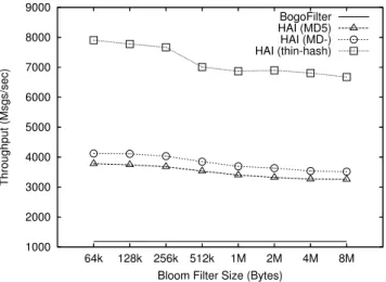
1000 2000 3000 4000 5000 6000 7000 8000 9000 8M 4M 2M 1M 512k 256k 128k 64k Throughput (Msgs/sec)
Bloom Filter Size (Bytes) BogoFilter HAI (MD5) HAI (MD-) HAI (thin-hash)
Fig. 14. Filter Throughput vs. Bloom Filter Size (Intel P4 CPU=2.6GHz)
outcome is close to the outcome of a randomly generated message. Therefore, higher token misclassification rates tend to push an email (ham or spam) score toward 0.5, and both the false positives and false negatives results exhibit a significant change at threshold 0.5, no matter what Bloom filter sizes are used.
The false negative rate, which is measured over spam messages, is shown at the right half of Figure 13. The false negative result is similar to the false positive result in the sense that larger Bloom filter size gives closer results to the original bogofilter, and filters smaller than 512KB differ from bogofilter more significantly than those with a larger than 512KB bit-vector. Furthermore, compared to false positive, the results of false negatives show a relatively larger gap between the bogofilter outcome and HAI filter, even with a large bit-vector at 16MB. We believe this is due to the quantization errors. A closer look at various quantization levels is presented later in this section. The accuracy results for HAI certainly also depend on the test data set as well as the training data set. We discuss the effect of the training data set on the HAI filter accuracy in a later section.
E. Effect of Hash Functions
We consider two aspects of hash functions, the hash com-plexity and the number of hash functions, for the HAI filter performance. We compare three hash functions: MD5, MD-and the one we built from scratch(thin-hash).
• MD5is picked to represent the well-known cryptographic
hash functions that provide a well distributed hash output. We use the standard implementation of MD5 [24].
• MD-is a simplification of standard MD5 implmentation. The core of MD5 is a combination of 4 “bitwise parallel” functions named F, G, H, and I. MD- only uses the F function.
• Thin-hashis a hash function that mixes the input token bytes with shift and xor bitwise operations. To generate a hash value, each byte of the token conducts 4 shift op-erations and is combined with previous bytes succesively
0 20 40 60 80 100 0 0.2 0.4 0.6 0.8 1
False Positive (Percentage)
Threshold Bogofilter 64k 128k 256k 512k 16M 0 20 40 60 80 100 0 0.2 0.4 0.6 0.8 1
False Negative (Percentage)
Threshold Bogofilter 64k 128k 256k 512k 16M
Fig. 13. Filter Accuracy vs. Bloom Sizes (h=4, q=8) Results with 1MB to 8MB bit-vectors are all between the results of 512KB and 16MB and thus not shown in the Figure
0 20 40 60 80 100 0 0.2 0.4 0.6 0.8 1
False Positive (Percentage)
Threshold Bogofilter HAI (MD5) HAI (MD-) HAI (thin-hash) 0 20 40 60 80 100 0 0.2 0.4 0.6 0.8 1
False Negative (Percentage)
Threshold Bogofilter
HAI (MD5) HAI (MD-) HAI (thin-hash)
Fig. 15. Filter Accuracy vs. Hash Algorithms (m=1MB, h=4, q=8)
by using xor operations and add operations. Thin-hash takes less than half the number of instructions as MD5. The detailed descriptions of these hash functions are presented in the extended version [31] of this paper. The throughput result is presented in Figure 14, which shows that MD- based HAI filter achieves about 10% higher throughput than the MD5 based filters. By using our own hash function, we achieve 95% throughput improvement comparing to MD5 based filters. For accuracy measurement, the false positive rates are close to identical for all the three hash functions. The false negative results for MD5 and MD- are also very close to each other. Thin-hash function displays worse false negative results than the other two. We believe the reason that thin-hash and MD-have worse false negative rate than MD5 is due to the hash conflicts. MD5 has fewer hash conflicts than the other two. This result is demonstrated in Figure 15. The result also indicates the trade-off between throughput and accuracy. A much simpler hash function can reduce the cost of hash computation with sacrifices on the accuracy.
We also investigate the effect of using a different number of hash functions. Using a small number of hash functions
reduces the number of marked bits, but has a higher probability of hash conflicts. Meanwhile using a large number of hash functions causes too many bits set in a Bloom filter with a limited bit-vector size and affects the accuracy. Figure 16 shows the filter accuracy results when using different numbers of hash functions. The bogofilter false negative result is also shown in the figure as a reference. Only the false negative result is shown here because the false positive results are all zero. For the size of 512K byte Bloom filter, Figure 16 demonstrates that the best choice is to use 8 hashes, with both 4 and 16 hashes having very close results.
F. Effect of Quantization Levels
This section presents the experimental results on the effect of quantization level selection. The results were obtained in two steps. First, we isolated the effect of quantization from Bloom filter misclassifications. To study the quantization effect alone, we applied it directly to bogofilter by quantizing all its statistical data in the database, and then measured its accuracy. Second, we did experiments with HAI filters with different quantization levels.
0 20 40 60 80 100 0 0.2 0.4 0.6 0.8 1
False Positive (Percentage)
Threshold Bogofilter Random (512k) Aggressive (512k) Conservative (512k) Random (192k) Aggressive (192k) Conservative (192k) 0 20 40 60 80 100 0 0.2 0.4 0.6 0.8 1
False Negative (Percentage)
Threshold Bogofilter Random (512k) Aggressive (512k) Conservative (512k) Random (192k) Aggressive (192k) Conservative (192k)
Fig. 18. Filter Accuracy vs. Value Selection Strategies for Multi-bit Marking (m=512KB, h=4, q=8)
0 20 40 60 80 100 32 16 8 4 2
False Negative (Percentage)
Number of Hash
Bogofilter HAI
Fig. 16. Filter Accuracy vs. Number of Hash Functions (m=512KB, q=8 bit, thresh=0.6)
Figure 17 compares the filter accuracy among three cases: the original bogofilter, bogofilter with quantizations, and HAI filters, with the number of quantization bits set from 2 to 16. Quantization introduces errors to data representation, which in general reduces filter accuracy. The original bogofilter’s accuracy result is used as the best-case reference to compare the performance of filters with various quantization levels. As expected, for bogofilters with quantization, 16 bits quantiza-tion performs best, but a quantizaquantiza-tion level around 4 to 8 is also close to the original non-quantized case. However, for HAI filters, higher quantization levels no longer produce the closest accuracy results to bogofilter. Instead, a quantization level at 8 shows the best accuracy results. By inspecting the token misclassification rate (by comparing each token outcome to bogofilter outcome), we found that the token misclassification rate increases as more quantizing bits are used. The best quantization level has to be one that balances the quantization error and the misclassification rate. For the given experiment setup, the best quantization level is 8. Similar to the effect of Bloom filter size, the optimal selection depends on the number of tokens to be stored. Nevertheless, an important
0 20 40 60 80 100 16 8 4 2
False Negative (Percentage)
Quantization Level
Bogofilter (with Quantization) Bogofilter HAI
Fig. 17. Filter Accuracy vs. Quantization Levels (m=512KB, h=4, thresh=0.6)
outcome from these experiments is that we have shown a small quantization level can effectively produce a filter accuracy that is very close to the accuracy of the original bogofilter.
G. Strategy for Handling Multi-bit Markings
In this section, we consider the strategies for handling the multi-bit marking error that is unique to the value retrieving extension of Bloom filter. When multi-bit marking occurs, the Bloom filter has to make a decision on the final lookup outcome. We consider three strategies for choosing the value. 1) Aggressive Strategy: every time multi-bit marking occurs, we always choose a value which indicates the highest spam-miness; 2) Randomly Selecting Strategy: randomly pick one value; 3) Conservative Strategy: we always choose a value which indicates lowest spamminess. Figure 18 shows the effect of different strategies on two Bloom filter sizes, 192KB and 512KB, respectively.
Figure 18 shows the effect of these three strategies for HAI under two different sizes: 192KB and 512KB. The two sizes are chosen to illustrate the impact of strategies under high and low multi-bit marking errors. Equation 10 indicates that
0 20 40 60 80 100 0 0.2 0.4 0.6 0.8 1
False Positive (Percentage)
Threshold
HAI with Query + Scoring HAI with Query + Pruning HAI with Query + Pruning + Scoring HAI with Query
0 20 40 60 80 100 0 0.2 0.4 0.6 0.8 1
False Negative (Percentage)
Threshold HAI with Query + Scoring HAI with Query + Pruning HAI with Query + Pruning + Scoring HAI with Query
Fig. 19. Filter Accuracy with Approximations in pruning and scoring stages(large bit-vector: 1MB, Quantization Level: 8, Hash Number: 4)
the probability for multi-bit marking error is high when the Bloom filter size is small. When Bloom filter size is small (here 192KB) the aggressive strategy always has lower false negative rate than the other two. Meanwhile false positive should follow the reverse trend of the false negative. The aggressive strategy results show a very different false positive measurement compared to bogofilter for any threshold less than 0.5. The conservative strategy gives the best result in the false positive measurement and has about the same false posi-tive as bogofilter. The random selection strategy is somewhere between but much closer to the aggressive approach.
But for larger bit-vectors (here 512KB), the differences among strategies are small. This is because the overall multi-bit marking error is small. All three strategies lead to very low false positives. Users can retain conservative strategy but still preserve a high filter accuracy. Overall this result indicates that the multi-bit handling strategies do not affect the filter accuracy in a significant way for large bit-vectors. However, to avoid false positives, we still recommend and use the third strategy in all other experiments.
H. Impacts of Approximations in the Pruning and the Scoring Stages
All previous HAI accuracy studies focus on the query stage only with fast pruning and fast scoring disabled. In practice, all three stages could introduce classification errors. In this section, we study the impacts of fast pruning and fast scoring on filter accuracy. The HAI filter accuracy with different setups are presented in Figure 19. The four setups are:1) HAI with Query, where we setup the HAI with only approximate lookup enabled. 2)HAI with Query + Pruning, which is the HAI filter with approximate pruning and approximate lookup enabled. 3) HAI with Query + Scoring, which is the HAI filter with approximate lookup and approximate scoring enabled. 4)HAI with Query + Pruning + Scoring, which is the HAI with all three approximations enabled. The result in Figure 19 shows that false positive rates remain identical. The false negative rates are very close and have no significant difference. This matches with our expectation that the main error introduced by the overall approximation comes from the approximate lookup.
V. RELATEDWORK
Message classification is a well-studied topic with applica-tions in many domains. This section makes a brief description of the related work in two categories: classification techniques for anti-spam purpose, and fast classification techniques using Bloom filters.
A. Anti-SPAM Techniques
Anti-spam is a very active area of research, and various forms of filters, such as white-lists, black-lists [6], [16], and content-based lists [13] are widely used to defend against spam. White-list based filters only accept emails from known addresses. Black-list filters block emails from addresses known to send out spam. Content-based filters make estimations of spam likelihood based on the text of that email message and filter messages based on a pre-selected threshold. Most of content-based filters use a Bayesian algorithm [13] to estimate message spamminess, and have been used in many spam filter products [15]. Recently, there have been several proposals about coordinated real-time spam blocking, such as the distributed checksum clearing house [26]. Most of these spam filters focus on improving the spam filtering accuracy. The work presented in this paper differs from them by investigating the accuracy-speed tradeoff. We have shown that with a carefully chosen algorithm, Bayesian filters can gain throughput with only a small loss on false negative rates. Many assumptions used by Bayesian filters to combine indi-vidual token probability for an overall score, such independent tokens, are not true for email messages, and more sophisticated classification techniques, such as k-nearest neighbors. In prac-tice, naive Bayesian classifiers often perform well [21], [23], [27], [30], and the current state of spam filtering indicates that they work very well for email classifications. Nevertheless, the work presented in this paper is to speedup the probability lookup stage for the probability calculation, and we expect the approach is applicable toward other classification techniques.
B. Bloom Filters Based Applications
Hash-based compressed data structure has recently been applied in several network applications, including IP traceback [28], traffic measurements [10] and fast IP packet classifica-tions [5]. For traffic measurement and traceback applicaclassifica-tions, Bloom filters are used to collect packet statistics and very often using hardware-based Bloom filters [7]. Bloom filter has also been adopted to build the proxy cache for the large scale web caching sharing protocol [11].The work presented in this paper uses Bloom filter to improve software processing speed, and investigate the trade off between throughput and accuracy. Among all these previous Bloom filter applications, the closest related work is the high speed packet classification using Bloom filter, which first studied the tradeoff between accuracy and the processing speed. This previous study uses bloom filter for membership testing, the work in this paper uses an extended bloom filter that supports value retrieving.
Bloom filter based technique has also been applied to collaborative spam filtering [17]. Our approach differs from previous approaches by providing a more general scheme for approximate data retrieval that can support arbitrary data value range. We also considered an additional level of approximation by applying lossy encoding to data representations. Moreover, this paper provides extensive studies on the impacts of var-ious system parameters, which are novel compared to other previous works.
VI. CONCLUSIONS
In this paper, we have explored the benefit of using approxi-mate classification to speed up spam filter processing. Using an extended Bloom filter to make approximate lookup and lossy encoding to approximately represent the statistic training data, we demonstrate close to an order of magnitude of speed up over two well-known spam filters. The result also shows that with careful selection of Bloom filter parameters, the errors introduced by the approximation becomes very small and the high speed filter with approximation can achieve very similar false positive and false negative rates as normal Bayesian filters.
The proposed extended Bloomfilter demonstrates the trade-off between the accuracy and the speed. In different from the traditional Bloomfilter, this extension is applicable for data retrieval. Although the nature of approximations prevents this scheme from being applied to the applications that require pre-cise data retrieval, our experiences in this paper indicate that it can benefit the applications that have speed demands and are resilient to a low retrieval error rate. We are currently exploring the feasibility to apply the scheme to other statistical-based applications, such as risk management, and reputation-based filtering.
REFERENCES
[1] “Quantizing for minimum distortion,”IEEE Transactions on Information Theory, vol. vol.28, no. 2, pp. 7–12, 1960.
[2] T. Berger and J. D. Gibson, “Lossy source coding,”IEEE Transactions on Information Theory, vol. vol.44, no. 6, pp. 2693–2723, 1998. [3] B. Bloom, “Space/time Trade-offs in Hash Coding with Allowable
Errors,”Communications of the ACM, vol. vol.13, no. 7, July 1970.
[4] A. Broder and M. Mitzenmacher, “A survey of network applications of bloom filters,”Internet Mathmatics, vol. vol.1, no. 4, pp. 485–509, 2004. [5] F. Chang, K. Li, and W. Feng, “Approximate packet classification
caching,” inProceedings of IEEE Infocom 2004, March 2004. [6] M. Delio, “Not All Asian E-Mail is Spam,” inWired News Article, Feb
2002, http://www.wired.com/news/politics/0,1283,50455,00.html Last accessed Feb 26, 2006.
[7] S. Dharmapurikar, P. Krishnamurthy, and D. E. Taylor, “Longest prefix matching using bloom filters,” inin Proceedings of ACM SIGCOMM 2003, August 2003, pp. 201–212.
[8] End-to-End Interest Research Group, “The end2end-interest archives,” http://www.postel.org/pipermail/end2end-interest/ Last accessed Feb 27, 2006.
[9] O. Erdogan and P. Cao, “Hash-av: Fast virus signature scanning by cache-resident filters,” in in Proceedings of Globecom’05, November 2005.
[10] C. Estan and G. Varghese, “New Directions in Traffic Measurement and Accounting,” inProceedings of Internet Measurement Workshop, November 2001, pp. 75–80.
[11] L. Fan, P. Cao, J. Almeida, and A.Z.Broder, “Summary cache: a scalable wide-area web cache sharing protocol,”IEEE and ACM Transaction on Networking, vol. 8, no. 3, pp. 281–293, 2000.
[12] D. Gall, “MPEG: A video compression standard for multimedia appli-cations,” April 1991, pp. 46–58.
[13] P. Graham, “A Plan for Spam,” Janurary 2003, in the Frist SPAM Conference http://spamconference.org.
[14] D. Heckerman and M. P. Wellman, “Bayesian networks,” no. 3, March 1995, pp. 27–30.
[15] S. Holden, “Spam filter evaluations,” http://sam.holden.id.au/writings/ spam2/ Last accessed Nov 2, 2005.
[16] P. Jacob, “The Spam Problem: Moving Beyond RBLs,” 2003, http: //theory.whirlycott.com/∼phil/antispam/rbl-bad/rbl-bad.html Last
ac-cessed Feb 26, 2006.
[17] P. L. C. Jeff Yan, “Enhancing collaborative spam detection with blom filters,” inProceedings of the 22nd Annual Computer Security Applica-tions Conference, 2006, pp. 414–428.
[18] P. Judge, “The SPAM Archive,” http://www.spamarchive.org Last ac-cessed Feb 26, 2006.
[19] K. Li, F. Chang, W. chang Feng, and D. Burger, “Architecture for packet classification caching,” inProceedings of IEEE ICON’2003, May 2003. [20] D. Lowd and C. Meek, “Good Word Attacks on Statistical Spam Filters,” inProceedings of the Second Email and SPAM conference, July 2005. [21] T. Meyer and B. Whateley, “SpamBayes: Effective open-source,
Bayesian based, email classifications,” inProceedings of the First Email and SPAM conference, July 2004.
[22] Perl Monger Users, “Perl monger mailing-list,” http://mail.pm.org/ pipermail/classiccity-pm/ Last accessed Feb 27, 2006.
[23] E. S. Raymond, “Bogofilter: A fast open source bayesian spam filters,” http://bogofilter.sourceforge.net/ Last accessed Nov 2, 2005.
[24] R. Rivest, “The MD5 Message-Digest Algorithm,” RFC 1321, April 1992.
[25] G. Robinson, “A statistical approach to the spam problem,” in Linux Journal 107, March 2003, http://www.linuxjournal.com/article.php?sid= 6467 Last accessed Nov 2, 2005.
[26] V. Schryver, “Distribute spam clearinghouse,” http://www.rhyolite.com/ anti-spam/dcc/ Last accessed Nov 2, 2005.
[27] M. Sergeant, “Internet level spam detection and spamassassin,” in
Proceedings of the 2003 Spam Conference, January 2003.
[28] A. Snoeren, C. Partridge, L. Sanchez, C. Jones, F. Tchakountio, S. Kent, and W. Strayer, “Hash-based IP Traceback,” in Proceedings of ACM SIGCOMM’01, August 2001.
[29] G. L. Wittel and S. F. Wu, “On Attacking Statistical Spam Filters,” in
Proceedings of the First Email and SPAM conference, July 2004. [30] A. Wood, “Quick spam filter,” http://freshmeat.net/projects/qsf/ Last
accessed Nov 2, 2005.
[31] Z. Zhong and K. Li, “Speed Up Statistical Spam Filter by Approximation,” Computer Science Department at the University of Georiga, Tech. Rep. 10-001, January 2010. [Online]. Available: http://www.cs.uga.edu/∼kangli/src/TR-10-001.pdf