Species Distribution Modeling
Jennifer Miller*
Department of Geography and the Environment, University of Texas at Austin
Abstract
The use of species distribution models (SDM) to map and monitor animal and plant distributions has become increasingly important in the context of awareness of environmental change and its ecological consequences. From their original inception as resource inventory and conservation mapping tools, SDM have evolved along with the increasing variety and availability of statistical methods, digital biological, and environmental data with which they are built in a geographic information system. Beyond predicting species distributions, these models have become an impor-tant and widely used decision-making tool for a variety of biogeographical applications, such as studying the effects of climate change, identifying potential protected areas, determining locations potentially susceptible to invasion, and mapping vector-borne disease spread and risk. This article outlines the steps involved in formulating an SDM and focuses on the conceptual and theoretical foundations on which it is based and identifies issues that have merited recent and will merit future research attention.
Introduction
An understanding of how and why biological organisms are distributed in space is a cen-tral tenet of biogeographical research. Species distribution models (SDM) quantify the correlation between environmental factors and the distribution of plant, and accordingly animal, species. This empirically derived ‘environmental profile’ can be used to describe and measure the importance of specific factors and to predict species’ distribution across unsampled areas, as well as to examine environmental change and its ecological conse-quences (Elith and Leathwick 2009; Franklin 1995, 2010; Guisan and Thuiller 2005; Guisan and Zimmermann 2000; Miller and Rogan 2007). In fact, the importance of bet-ter understanding the relationship between organisms and their environment was recently identified as one of the five ‘grand challenges’ in organismal biology (Schwenk et al. 2009).
This type of correlative predictive modeling in general has a long history in both geog-raphy and ecology, and recent growth has been further spurred by developments in geographic information systems (GIS) and related technologies, resulting in both greater availability of digital data and a wider variety of tools with which to analyze them. As a result of concurrent development of similar applications with slightly different objectives, the process referred to here as species distribution modeling has been described formerly as ‘predictive vegetation mapping’ (Franklin 1995), ‘predictive habitat distribution model-ing’ (Guisan and Zimmermann 2000), ‘bioclimatic envelope modelmodel-ing’ (Pearson and Dawson 2003), ‘habitat suitability index mapping’ (Clark et al. 1993), ‘habitat suitability modeling’ (Hirzel and Le Lay 2008), and ‘niche modeling’ (Stockwell 2006), among other terms. The distinction between the words ‘map’ and ‘model’ reflects a subtle difference in emphasis from the product (map) to the process (model). An even more
important distinction between the related concepts of ‘habitat’ and ‘niche’ is addressed in the next section.
The terminology seems to be converging on ‘species distribution model’, although it is technically the distribution of suitable environmental factors that is modeled⁄mapped (see Franklin 2010; Kearney 2006). This generalization also makes these models appropriate for studying the distribution of related biogeographical variables such as communi-ties⁄assemblages (Ferrier et al. 2002), species richness (Jetz and Rahbek 2002), invasive species potential (Richardson and Thuiller 2007), and disease vectors (Peterson 2006).
In addition, SDM have been used for conservation planning (Arau´jo et al. 2002), to test biogeographical hypotheses (Leathwick 1998), investigate evolutionary processes (Kozak et al. 2008), identify suitable areas for species re-introduction (Engler et al. 2004), map fuels and fire regimes (Rollins et al. 2004), and increase detection likelihood of rare species (Edwards et al. 2005). In a prediction context, the models can be used in two ways: interpolation to unsampled sites in the same general time frame and region where environmental conditions are similar; and extrapolation to past or future time frames (also called forecasting) or sites outside of the region in the same time frame (also called trans-ferability) (Elith and Leathwick 2009). Limitations associated with using SDM for extrap-olation are discussed in a subsequent section.
In this study, I review the theoretical background of SDM, outline the steps involved in making an SDM, and identify issues and applications associated with new develop-ments in the field.
SDM Background
SPECIES’ RESPONSE TO ENVIRONMENTAL GRADIENTS
The concept of a species’ ecological niche provides the central theoretical basis for describing species–environment relationships in SDM. Despite being a core idea in ecol-ogy, ‘niche’ is not an unambiguous term and much has been written about its different interpretations, both in general (see Chase and Leibold 2003; Pulliam 2000) and as it applies to SDM in particular (Arau´jo and Guisan 2006; Austin 2002; Franklin 2010; Gui-san and Zimmermann 2000; Hirzel and Le Lay 2008; Kearney 2006; Sobero´n 2007). Hutchinson’s (1957, 416) definition of a species’ niche as an ‘n-dimensional hypervo-lume’ in environmental space in which the species can exist indefinitely is the one most widely used in an SDM context. This definition is further refined to differentiate between the fundamental niche, the range of environmental conditions a species is physi-ologically able to tolerate, and the realized niche, the subset of the fundamental niche actually occupied as a result of biotic interactions.
However, the nature and spatial scale of these biotic interactions are somewhat prob-lematic – Arau´jo and Guisan (2006) suggest that Hutchinson intended only negative interactions, specifically competition, to define the realized niche, whereas positive inter-actions such as mutualism would comprise the hypervolume defining the fundamental niche. These interactions often occur at spatial scales too fine to be effectively resolved in most SDM studies. In addition, biotic processes like dispersal are often equally important factors (even at coarser spatial scales), but their temporal nature makes them incompatible with Hutchinson’s more static niche concept (Arau´jo and Guisan 2006; Sobero´n 2007). It is important to be very clear about what exactly is being modeled⁄mapped in a particular SDM application, and the assumptions and limitations associated therein. Although the ecological niche concept is integral to species distribution modeling, the term ‘habitat’
more accurately describes what is most often modeled in SDM. Addressing the somewhat muddled terminology, Kearney (2006) frames the two terms in a hierarchy, with ‘niche model’ resulting from a more mechanistic analysis that addresses a species’ morphology, physiology, behavior, and the way in which a species interacts with its environment. A habitat map results from the descriptive⁄correlative analysis using generally environmental factors that is associated with most SDM studies.
Each environmental gradient can be considered a single dimension in Hutchinson’s
n-dimensional niche, and the species’ response to the environmental conditions along the gradient defines its distribution in environmental space. The shape of a response curve relates some measure of species importance (abundance, occurrence) to the gradual change in availability of resources or physiological tolerances along the gradient, and is typically characterized by minimum and maximum thresholds, as well as an optimum (or mode) where the importance measure reaches its height.
The type of environmental gradients used is an important consideration when formu-lating SDM. Austin (1980) classified the two most important environmental gradients used in SDM as direct, which have a direct physiological effect on species growth but are not consumed (e.g. temperature, pH), and resource, which are used or consumed (e.g. water nutrients). Sobero´n (2007) suggests that these types of factors can be differentiated by spatial scale: direct variables are more often available at coarser scales and used to describe species’ habitat; as resource variables are consumed, their use implies potential for competition and they are necessarily measured and exert influence at finer scales. A third type of gradient isindirect, which results from location-specific correlations (e.g. ele-vation, latitude).
It is also important to clarify how these ecological niche concepts are translated in the species distribution modeling process. A simple way of relating the concept of an ecologi-cal niche to SDM is that the niche describes a species’ fitness in environmental space, a statistical method quantitatively describes that environmental profile, and the resulting predicted map translates the environmental profile into some measure of suitability in
geographic space. The relationship between environmental space and geographic space is addressed in more detail in the next section.
ENVIRONMENTAL VERSUS GEOGRAPHIC SPACE
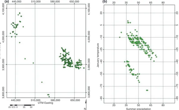
It is worth emphasizing here that both the niche concept and gradient analysis describe the distribution of a species in environmental space. The utility of SDM (and its GIS component) lies in translating this species–environment relationship into geographic space. This is illustrated in Figure 1 using data on Yucca brevifolia occurrence in the Mojave Desert, CA (see Miller and Franklin 2006 for data description), and a simple two-dimensional environmental profile. Figure 1A shows the distribution of Y. brevifolia
in geographic space (Universal Transverse Mercator (UTM) easting and northing), and Figure 1B shows the same data distributed in two-dimensional environment space (summer precipitation and minimum January temperature). Presumably the two ‘patches’ in which Y. brevifolia occurs in geographic space (Figure 1A) have similar environmental conditions in addition to the two dimensions represented in Figure 1B.
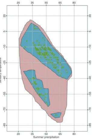
Hypothetical examples of the fundamental and realized niche are drawn around the actual species data in Figure 2. The fundamental niche (red) describes the range of Janu-ary temperature and summer precipitation conditions within which Y. brevifolia can persist. The realized niche (blue) describes the subset of those conditions Y. brevifolia
interactions such as competition, dispersal limitations, or abiotic factors such as distur-bance. The (green) points show actual observations of Y. brevifolia, all of which must be within the realized niche, although there are parts of the realized niche with no observa-tions because of sampling effort or detectability. The environmental profile of Y. brevifolia
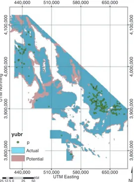
can be quantified using a modeling algorithm (discussed below), then combined with GIS layers of the environmental variables to produce a geographic distribution of suitable species’ habitat. This is shown in Figure 3, with fundamental niche now translated as potential distribution and realized niche translated as actual distribution. Another distinc-tion is that the fundamental niche in environmental space (Figure 2) is static, whereas the potential distribution (Figure 3) can vary as a function of changing environmental condi-tions.
Strictly speaking, as SDM are based on observed data (which can be affected by biotic interactions, disturbance, dispersal limitations, etc.), the mapped potential distribution is not exactly the same as the fundamental niche, and unless there are variables that repre-sent biotic interactions or disturbance, the actual distribution is not exactly coincident with the realized niche. This process is covered in more detail next.
SDM Process
In a comprehensive review, Guisan and Zimmermann (2000) outlined the steps involved in species distribution modeling. They emphasized the importance of incorporating ecological theory in every step of the process; from conceptualizing models based on an assumption of species–environment pseudo-equilibrium to specifying ecologically realistic response curves (also see Austin 2002; Guisan and Thuiller 2005). The types of data and modeling algorithm used determine what kind of map is produced, so the overall
(a) 440,000 (b) 440,000 510,000 580,000 UTM Easting UTM Nor thing 650,000 4,100,000 4,000,000 3,900,000 3,800,000 4,100,000 4,000,000 3,900,000 3,800,000 510,000 580,000 650,000 20 20 5 –10 –25 –40 –55 –70 –85 20 5 –10 –25 –40 –55 –70 –85 35 50 65 80 20 35 50 65 80 Summer precipitation 25 12.5 0 25 50KM J a n uar y temper ature N
Fig. 1. (a) Distribution ofYucca brevifolia in geographic space (UTM easting and northing); (b) distribution ofY. brevifoliain two-dimensional (summer precipitation and January temperature) environmental space.
objective should be the factor that informs each of these steps and decisions. Heikkinen et al. (2006) describe how decisions and assumptions associated with data and methods can impact map predictions in a climate change modeling context.
An overview of the species distribution modeling process is given in Figure 4. As an extensive discussion of each of these different components is beyond the scope of this review, I will briefly describe each step, focusing on data and methods most commonly used in SDM and associated ‘best practices’.
BIOLOGICAL DATA
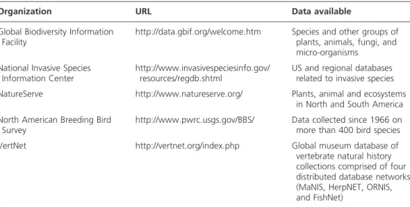
Biological data that describe the distribution of a species (see Table 1 for sources) can be measured at nominal (e.g. presence⁄absence, type), ordinal (e.g. ranked abundance) and ratio (e.g. abundance, richness) levels, which impacts which types of modeling algorithms are appropriate to use, and subsequently the measurement level of the SDM product (e.g. probability or suitability of occurrence, type, expected mean).
For adequate analytical power, a ratio of ten observations for every predictor variable is considered a minimum when constructing a modeling dataset (Vaughan and Ormerod
20 35 50 65 80 20 35 50 65 80 Summer precipitation 20 5 –10 –25 –40 –55 –70 –85 20 5 –10 –25 –40 –55 –70 –85 J a n u ar y temper ature
Fig. 2. A hypothetical example of the fundamental niche (red) and the realized niche (blue) in (real) two-dimen-sional environmental space. Red is the part of the fundamental niche (potential distribution) not occupied as a result of disturbance, competition, dispersal limitations, historical barriers, etc. Blue is the realized niche (actual dis-tribution) the subset of the fundamental niche actually occupied, including observed occurrences (green circles) as well as unobserved.
2003), although this ratio can be affected by spatial autocorrelation (Miller et al. 2007) and multicollinearity. Franklin (2010) suggests a sample size that results in a ratio of 20 to 1, and even 40 to 1 when using stepwise regression. An additional consideration with presence⁄absence data is prevalence, the ratio of ‘presence’ to ‘absence’ in the dataset. The sensitivity of some accuracy metrics to prevalence has been studied (Manel et al. 2001), and when prevalence-independent metrics are used, even prevalence (close to 0.5) has been associated with more accurate predictive models (e.g. McPherson et al. 2004), whereas other studies have shown rare species (low prevalence) to be more accurately modeled than more prevalent species, owing to their often stronger environmental corre-lations (Franklin et al. 2009; Segurado and Arau´jo 2004).
The species data most relevant to describing habitat suitability will have been collected across a broad range of environmental and geographic space. Environmental gradients have been used to design sampling strategies appropriate for increasing the floristic diver-sity sampled (Franklin et al. 2001) and for increasing the detection of rare species (Edwards et al. 2005). However, more recent efforts have focused on maximizing the utility of existing data already compiled by museums or natural history collections (Elith et al. 2006). The limitations of these data, typically presence-only and based on biased, opportunistic sampling strategies, are somewhat offset by their proliferation. Lacking observations of absence makes these data unsuitable for many of the commonly used SDM algorithms and model assessment techniques, unless ‘pseudo-absences’ are assigned to unsampled portions of the study area. In fact, methods used to generate pseudo-absences and their effects on model performance have been the sole focus of recent stud-ies (e.g. Chefaoui and Lobo 2008; Engler et al. 2004).
440,000 Actual Potential 510,000 580,000 650,000 4,100,000 4,000,000 3,900,000 3,800,000 4,100,000 4,000,000 3,900,000 3,800,000 440,000 510,000 580,000 650,000 p yubr UTM Easting UTM Nor thing N KM 25 12.5 0 25 50
Fig. 3. This is the two-dimensional environmental profile from Figure 2 translated into geographic space. Funda-mental niche is mapped as potential habitat and realized niche is mapped as actual habitat; actual observations are green circles.
Fig. 4. Species distribution modeling process.
Table 1. Sources of biological data used as response variable in species distribution model.
Organization URL Data available
Global Biodiversity Information Facility
http://data.gbif.org/welcome.htm Species and other groups of plants, animals, fungi, and micro-organisms
National Invasive Species Information Center
http://www.invasivespeciesinfo.gov/ resources/regdb.shtml
US and regional databases related to invasive species NatureServe http://www.natureserve.org/ Plants, animal and ecosystems
in North and South America North American Breeding Bird
Survey
http://www.pwrc.usgs.gov/BBS/ Data collected since 1966 on more than 400 bird species VertNet http://vertnet.org/index.php Global museum database of
vertebrate natural history collections comprised of four distributed database networks (MaNIS, HerpNET, ORNIS, and FishNet)
In addition to potential location and identification errors, there are several uncertainty issues associated with the biological data used in SDM. The ambiguous nature of absence data has been addressed under the auspices of ‘detectability’ – that is a species may exist in an area but remain unobserved because it is mobile or cryptic, typically a more com-mon problem with animal species but even plant species can have detection problems related to seed banks and seasonal differences (Edwards et al. 2005; Franklin 2010; Wintle et al. 2004). Additionally, a correct observation of ‘absent’ that occurs in suitable habitat as a result of biotic interactions, dispersal limitations, disturbance, etc. may be problematic for model calibration.
ENVIRONMENTAL DATA
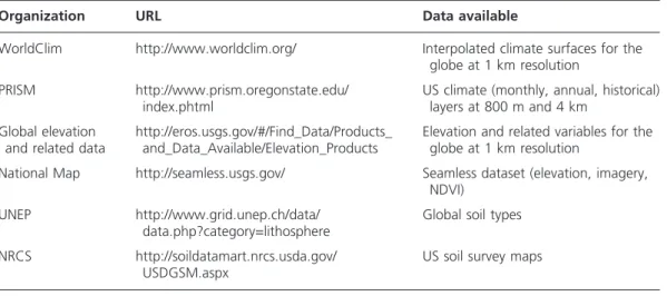
The next step in formulating an SDM is to obtain GIS layers of environmental variables that describe an appropriate combination of direct, resource, and indirect gradients (see Table 2 for sources). Climatic and topographical variables are the most widely used pre-dictors in SDM, as they describe broad-scale physiological tolerances related to water and temperature, and finer-scale spatial variation in site energy and moisture availability, respectively.
Climate data
Much has been written about climate and its effects on plant distribution (e.g. Holdridge, 1947, Holdridge, 1967). The geographic variation in temperature and availability of mois-ture and light is considered to be one of the most important factors determining which plants grow where. In a species distribution modeling context, climate variables can represent both direct (temperature) and resource (moisture) gradients as summary variables (e.g. annual precipitation) or more complex and presumably more ecologically relevant variables (e.g. seasonal extremes, humidity).
Although climate is indisputably important in determining species distributions, GIS climate layers are typically produced by interpolating ground station data and are of limited availability and quality for many areas (Parra et al. 2004). More recently, Hijmans Table 2. Sources of environmental data used as predictor variables in species distribution model.
Organization URL Data available
WorldClim http://www.worldclim.org/ Interpolated climate surfaces for the globe at 1 km resolution
PRISM http://www.prism.oregonstate.edu/ index.phtml
US climate (monthly, annual, historical) layers at 800 m and 4 km
Global elevation and related data
http://eros.usgs.gov/#/Find_Data/Products_ and_Data_Available/Elevation_Products
Elevation and related variables for the globe at 1 km resolution
National Map http://seamless.usgs.gov/ Seamless dataset (elevation, imagery, NDVI)
UNEP http://www.grid.unep.ch/data/ data.php?category=lithosphere
Global soil types
NRCS http://soildatamart.nrcs.usda.gov/ USDGSM.aspx
et al. (2005) derived a global dataset (http://www.worldclim.org/) available at several different spatial resolutions (30 seconds to 10 minutes) of nineteen different climate variables including annual trends, seasonality, and extreme or limiting factors. Most statis-tical methods are affected by multicollinearity, when predictor variables are highly corre-lated with each other, so ecological knowledge and a priori testing should be part of the model formulation. Data reduction methods such as principal component and factor anal-ysis can be used to reduce multicollinearity, often at the expense of interpretability.
Topography
Guisan and Zimmermann (2000) outline the many uses of digital elevation models in SDM: in addition to providing the basis for deriving more complex topographic vari-ables, they can be combined with geostatistics to interpolate climate station data; they can be used to stratify samples; and they can be used to georectify remotely sensed images.
As predictor variables, topographic variation is generally associated with micro-climate effects related to water availability, temperature, and incoming solar radiation. Although simple topographic variables that represent indirect gradients, such as elevation, slope, and aspect, should result in lower predictive accuracy when used along with direct and resource gradients as predictor variables, they are often empirically important as they tend to be derived with higher accuracy (Guisan and Zimmermann 2000; Rollins et al. 2004). More complex topographic variables, such as potential solar radiation, topo-graphic moisture index, and landscape position, can be calculated to describe some combination of soil properties related to depth, texture, and water-holding capacity (Franklin 1995). One general assumption has been that as the processing steps involved in deriving a topographic variable increase, so too does its propensity for error (Guisan and Zimmermann 2000), although Van Niel et al. (2004) show that this is not always the case. In a study that simulated error propagation in the derivation of topographic variables, they found that more complex variables, such as net solar radiation, were typ-ically less affected by error than comparatively simple variables, such as slope and aspect (Van Niel et al. 2004).
Other variables
In addition to climate and topography, other variables such as geology and soil type can also be used to represent moisture and nutrient availability, although usually at a coarser scale due to their categorical nature (at least in most available digital maps). More applica-tion-specific variables such as ‘distance to ____ (roads, water, edge, etc.)’ can be calcu-lated in a GIS to describe proximity to disturbance or important resources (Osborne et al. 2001). Distribution maps for other species have also been used as predictor variables to represent potential competition, predation (Leathwick and Austin 2001), or facilitation (Heikkinen et al. 2007), as well as to stratify sampling schemes aimed at increasing detec-tion of rare species (Edwards et al. 2005).
Remotely sensed data and landscape ecology metrics can be used to describe habitat structure, biophysical properties, landscape pattern, and heterogeneity (Aplin 2005; Gotts-chalk et al. 2005; Kerr and Ostrovsky 2003; Miller and Rogan 2007). Land-cover maps are the most often used remote sensing product, and they have improved the model per-formance when used hierarchically with climate at regional scales (Pearson et al. 2004); however, their inclusion in continental-scale predictions is often overwhelmed by the effect of bioclimatic variables (Thuiller et al. 2004). Land-use maps have been used to model the effect of human impact on gypsy moth spread (Lippitt et al. 2007). SDM
studies that use image spectral values and vegetation indices as predictors are less common outside of bird studies (see Gottschalk et al. 2005), but have improved models of rare early successional trees in Utah (Zimmermann et al. 2007).
MODELING ALGORITHMS
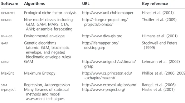
The number of algorithms available to statistically describe species–environment rela-tionships and software packages within which they are implemented is quite staggering (see Table 3 for an incomplete list). Although GIS and science provide a set of tech-niques and theory uniquely suitable for handling the types of spatial data used in SDM, the basic statistical analysis methods (e.g. linear regression) available as part of many GIS software packages are based on assumptions not appropriate for use with biogeographical data (e.g. independent observations, linear relationships between response and predictors). GIS is invaluable during the data input, management, and output stages, particularly for calculating new variables, such as more complex topo-graphic variables from elevation or ‘distance to ___’ variables. The statistical analysis is still largely carried out in stand-alone or user-written statistical software, the results of which (e.g. equations, rules) are subsequently integrated in a GIS to produce maps and related results.
Although habitat suitability maps have been produced quite successfully in the past using deductive models and expert knowledge (Scott et al. 1993), inductive models are far more frequently used in SDM now because of their replicability and relatively greater objectivity. A more extensive review of all of the different types of algorithms used in SDM is beyond the scope of this study (but see Elith et al. 2006; Franklin 2010; Guisan and Zimmermann 2000), therefore three categories of modeling methods most commonly used in SDM and key differences among them are briefly described here.
Table 3. Sources of software for species distribution model algorithms.
Software Algorithms URL Key reference
BIOMAPPER Ecological niche factor analysis http://www.unil.ch/biomapper Hirzel et al. (2001)
BIOMOD Nine model classes including
GLM, GAM, MARS, CTA, ANN; ensemble forecasting
http://r-forge.r-project.org/ projects/biomod/
Thuiller et al. (2009)
DIVA-GIS Environmental envelope http://www.diva-gis.org Hijmans et al. (2001) GARP Genetic algorithms
(atomic, GLM, bioclimatic envelope, and negated bioclimatic envelope rules)
http://lifemapper.org/ desktopgarp
Stockwell and Peters (1999)
GRASP GAM http://www.unige.ch/ia/climate/
grasp
Lehmann et al. (2002)
MaxEnt Maximum Entropy http://www.cs.princeton.edu/ ~schapire/maxent/
Phillips et al. (2006, 2009)
SAM Regression, Autoregression http://www.ecoevol.ufg.br/sam/ Rangel et al. (2006) R-project Many libraries of statistical
methods and model assessment techniques
The type of algorithm used should be based upon, among other things, the measure-ment level and characteristics of the biological data, the measuremeasure-ment level and volume of environmental data, and the desired map product. Although the outcomes of different SDM approaches can be similar, distinctions among modeling algorithms exist in terms of being more appropriate for predicting actual versus potential distribution (e.g. complex models using presence⁄absence data versus simple models using presence only data; Jime´nez-Valverde et al. 2008) as well as more subtle differences between predictions of probability (e.g. from logistic regression) versus suitability (e.g. from classification trees).
The first group of methods is related to traditional regression and includes general-ized linear models (GLM) and their non-parametric extension, generalgeneral-ized additive models (GAM), both of which can handle different measurement levels of the response variable by using a different link function (e.g. logistic for presence⁄absence, Poisson for count). GAM and a related method, multivariate adaptive regression splines (MARS), are more flexible than GLM as they are fit using smoothing and piecewise linear splines, respectively, and are particularly useful for identifying the shape of species’ responses (see Leathwick et al. 2005; Miller and Franklin 2002). MARS is computationally faster than GAM and the results are more easily converted to map predictions in a GIS; however, the algorithms currently used require normally distrib-uted error terms. This makes MARS unsuitable for use with presence⁄absence data unless the basis functions are extracted and used to parameterize a GLM (Franklin and Miller 2010; Leathwick et al. 2005). Recent research has focused on how spatial autocorrelation affects SDM and most of these spatial methods (e.g. autoregression, generalized linear mixed models) are related to generalized regression (see Dormann et al. 2007; Miller et al. 2007 for review).
More flexible ‘data-driven’ methods that are not based on specific distribution func-tions and do not require a priori model specification are typically categorized as machine-learning methods. These methods are related to supervised classification used in image processing and include decision trees, artificial neural networks, and genetic algorithms, and are also often useful in an exploratory context (see Franklin 2010). They partition observations along environmental space and, as a result, are considered ‘local’ as opposed to ‘global’ GLM that are fit using all observations and environmental data at the same time. Decision trees are particularly appropriate where there are hierarchical effects among predictors (e.g. the relationship between precipitation and aspect) and their prod-uct is more ecologically interpretable than many other machine-learning methods (see De’ath and Fabricius 2000).
Some of these methods, such as artificial neural networks, are iterative in nature, and there are a number of external iterative methods that can be applied to machine-learn-ing algorithms (most often decision trees) to improve accuracy. These ‘ensemble’ meth-ods (e.g. ‘bagging’, ‘boosting’, and Random Forests) generally involve developing multiple models on different subsets of the data, the results of which are averaged (Franklin 2010). A third group of methods developed to deal with presence-only data-sets includes environmental distance, similarity, and envelope methods such as Gower metric, Mahalanobis distance, and ecological niche factor analysis, all of which describe some measure of habitat suitability. More recently, generalized regression and machine-learning methods have been developed or extended to presence-only data, typically necessitating either the use of ‘background’ or the calculation of pseudo-absence data. Maximum entropy (Maxent; Phillips et al. 2006), a machine-learning method, has been very effective in SDM studies with presence-only data, particularly with small sample sizes (Phillips et al. 2005); however, its performance degrades when used for
extrapolation (Franklin 2010). Although absence data provide useful information on prevalence (Phillips et al. 2009), it can be misleading when a species is not in equilib-rium with the environment or when there is an historical or biotic barrier preventing it from occurring in suitable habitat. Presence-only data are most appropriate for predicting potential distribution (Jime´nez-Valverde et al. 2008), such as with invasive species or climate change impact applications.
Irrespective of the method used, some kind of model calibration is involved during which appropriate variables and their transformations are selected, some measure of model fit is optimized, and parameters are estimated. The calibration process can range from user-involved and subjective (GLM) to more automatic and objective (machine-learning methods). A final model is selected based on these metrics (e.g. AIC, D2, R2), but the model fitness cannot be compared using these metrics across different model types (see Model assessment section).
Despite a profusion of recent studies that compared different algorithms (Elith et al. 2006; Prasad et al. 2006; Segurado and Arau´jo 2004), no single method has emerged as consistently superior independent of species’ study area and sample characteristics. Instead, model accuracy has been correlated with species’ geographic distribution (Segurado and Arau´jo 2004), habitat specificity (Tsoar et al. 2007), species rarity (Franklin et al. 2009), and other ecological traits such as endemicism and migratory status (for birds; McPherson and Jetz 2007).
A related issue involves the variability in map predictions among different models (as well as within different models as a function of data partitioning schemes, model specifi-cation, etc.), particularly when used to guide policy decisions as in the case of climate change projections. A strategy borrowed from economics and weather forecasting involves combining many different predicted maps into a consensus or ensemble predic-tion (Arau´jo and New 2007; Marmion et al. 2009; Thuiller et al. 2009), which often increases accuracy while reducing uncertainty.
MODEL ASSESSMENT
Since species’ distribution maps (or some variation thereof) are the primary goal, it makes sense to focus on the accuracy of these maps as a standard comparison metric. This step involves assessing how well the model predictions compare with the actual observations and is also not without some uncertainty and subjectivity. A robust and rigorous measure of model accuracy involves using the model with independent data collected from a new area or based on a different sampling strategy (Guisan and Zimmermann 2000). As is often the case, if a truly independent dataset is not available, the modeling dataset (train) can be partitioned in ways to approximate an independent dataset (test). Fielding and Bell (1997) discuss many partitioning scenarios, ranging from leave-one-out jackknifing for smaller datasets (Pearson et al. 2007) to twofold partitioning, initially dividing the data into two datasets (for presence⁄absence datasets they suggest a ratio of [1 + (p ) 1)1⁄2])1, where p is the number of predictors, which equates to 75:25 train:test with more than ten predictors). Newer versions of SDM software facilitate k number of data splits (e.g. 1000) and the results to be averaged (BIOMOD; Thuiller et al. 2009).
The goodness-of-fit statistic used with the training data in the model calibration step described above (e.g. R2, D2) is rarely used with the test data during model assessment because it is not a measure that is comparable across different types of models. Instead, predictions are generated by combining the fitted model with the test data values, and these predicted values are compared with observed values. As the majority of SDM
studies involve presence⁄absence response data, this step is illustrating using examples for presence⁄absence data.
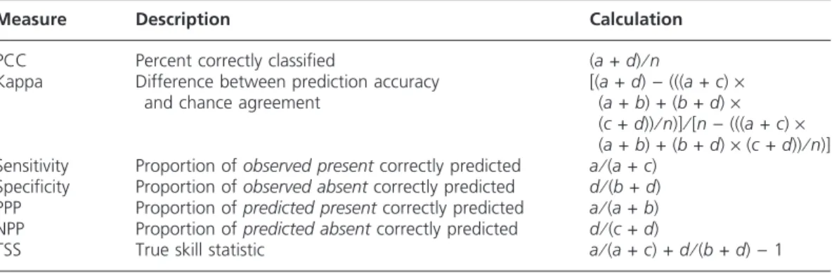
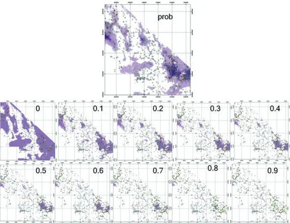
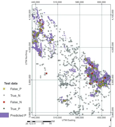
Two main types of accuracy metrics are used with presence⁄absence data. ‘Confusion matrix’ based metrics compare observed discrete cases to predicted discrete cases (Figure 5), and there are a number of ways of summarizing this information, such as kappa, percent correctly classified (PCC), sensitivity, specificity, and true skill statistic (TSS).(Table 4). As these methods deal with discrete predictions and most of the algorithms used with pres-ence⁄absence SDM generate continuous or somewhat continuous predictions (but see Peterson et al. 2008), a threshold must be selected above which cases are converted to ‘present’ and below which cases are ‘absent’. Threshold selection is not a trivial matter as it can have significant effects on both model accuracy and mapped predictions (see Figure 6 for GLM example). A threshold should be selected in accordance with the objectives of the study and two recent studies have suggested guidelines on which to base this decision, such as using the prevalence, the average predicted probability of the training data (Liu et al. 2005), or the threshold that maximizes kappa (Freeman and Moisen 2008).
The four elements of the confusion matrix are mapped along with predicted presence (based on a recommended threshold equal to the prevalence for the Y. brevifoliadata, 0.1) in Figure 7. In general, false-positives (commission errors) may result from biotic or abiotic factors that prevent a species from occupying suitable habitat, such as dispersal
Observed Pr edic te d Present Present Absent Absent a (TP) b (FP) c (FN) d (TN)
Fig. 5. Confusion matrix used to summarize classification accuracy for binary categorical data. Green boxes indicate correct results; red boxes indicate incorrect results.
Table 4. Common metrics used for binary species distribution model accuracy assessment.
Measure Description Calculation
PCC Percent correctly classified (a+d)⁄n
Kappa Difference between prediction accuracy and chance agreement
[(a+d))(((a+c)·
(a+b) + (b+d)·
(c+d))⁄n)]⁄[n)(((a+c)·
(a+b) + (b+d)·(c+d))⁄n)] Sensitivity Proportion ofobserved presentcorrectly predicted a⁄(a+c)
Specificity Proportion ofobserved absentcorrectly predicted d⁄(b+d) PPP Proportion ofpredicted presentcorrectly predicted a⁄(a+b) NPP Proportion ofpredicted absentcorrectly predicted d⁄(c+d)
limitations and historical barriers or from detection issues; false-negatives (omission errors) can result from data or model inaccuracies or even a threshold that was too high.
In addition to being threshold-dependent, many of these methods are also prevalence-dependent (except sensitivity and TSS), to varying degrees. PCC, negative predictive power (NPP), and positive predictive power (PPP) are all highly prevalence-dependent, whereas kappa is less so (Fielding and Bell 1997). Recent research has shown that kappa is unimodally related to variation in prevalence (Allouche et al. 2006) and Freeman and Moisen (2008) caution that kappa should not be used to compare models based on data for which prevalence differed significantly. Of the seven metrics listed here, only kappa and TSS compare model performance to chance classification and use information on both commission and omission errors (Allouche et al. 2006). Using simulated and real data, Allouche et al. (2006) showed that TSS is theoretically unaffected by prevalence and empirically has an inverse relationship that is consistent with an ecological interpretation of how prevalence might affect model accuracy.
Using data from a Y. brevifolia GLM (details of model in Miller and Franklin 2006), these accuracy metrics vary considerably across threshold value (Figure 8). NPP varies not only the least across thresholds (and along with PPP is analogous to user’s accuracy in remote-sensing classification), but is also typically one of the least important measures as it deals only with how many of the predicted absents are really absent. Sensitivity is typically very important (and along with specificity analogous to producer’s accuracy), Fig. 6. Probability-threshold process. These maps show the result from a generalized linear model (prob) and the binary presence⁄absence maps that result from different threshold selections.
and is only high at low thresholds that result in commission errors. Using the probability threshold closest to the prevalence of the data (0.1; see Liu et al. 2005), the accuracy metrics range from 0.43 (kappa) to 0.99 (NPP).
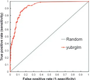
The second type of accuracy metric, receiver-operating characteristic (ROC), is both threshold- and prevalence-independent (Fielding and Bell 1997; Manel et al. 2001). Sensitivity is plotted against (1-specificity) for all available thresholds and the area under the curve shows how well the model can discriminate between two cases (Figure 9).
Measuring accuracy with ROC obviates the subjective step of selecting a threshold, a distinct advantage, and it also uses all of the information from the predictions, rather than just discretized results. Its relative nature makes it prevalence-independent and facilitates comparisons across many different algorithms and datasets. For these reasons, ROC has become the standard measure used to compare accuracy for different methods (Elith et al. 2006), despite its relatively new introduction to SDM (Fielding and Bell 1997).
However, criticisms of ROC as a robust accuracy measure have been lodged recently (see Lobo et al. 2008; Peterson et al. 2008). Peterson et al. (2008) suggest a modification that replaces the (1-specificity) x-axis with the proportion of the area predicted to be
440,000 510,000 580,000 650,000 4,100,000 4,000,000 3,900,000 3,800,000 4,100,000 4,000,000 UTM Nor thing 3,900,000 3,800,000 440,000 510,000 UTM Easting 580,000 650,000 N 25 12.5 0 25 50KM Test data False_P False_N True_N True_P Predicted P
Fig. 7. This illustrates how model accuracy is assessed. A threshold (0.1) is selected to convert continuous model predictions to predicted presence (purple) and predicted absence (white); Observed presence⁄absence cases from test data are compared with predicted presence⁄absence cases and the information is summarized in a confusion matrix (Figure 5) and subsequent accuracy metrics (Figures 8 and 9).
present, which has the added advantage of being suitable for use with presence-only datasets.
One point on which consensus seems to have been reached regarding SDM accuracy assessment is that no single method should be used alone. Each of the methods listed here and reviewed more extensively elsewhere (Allouche et al. 2006; Fielding and Bell 1997; Franklin 2010) has advantages and disadvantages and different levels of importance depend-ing on the objectives of the study. For example, sensitivity is far more important than specificity when dealing with conservation of rare species or potential for invasive species.
Summary and Conclusion
In a 2002 study, Austin noted the disconnection between statisticians and ecologists who do SDM research – the former are more likely to use highly sophisticated statistical tech-niques while failing to incorporate ecological theory, whereas the latter use ecological theory to develop relatively more basic models. More recently, Jime´nez-Valverde et al. Fig. 8. Variation in confusion matrix derived accuracy metrics across different thresholds forYucca brevifoliaGLM (see Figure 6 for maps).
Fig. 9. A receiver operating characteristic plot using the same data from Figure 8. The area under the curve is 0.93.
(2008) suggested that differences among simple and more complex model performance may result as much from conceptual misunderstanding as actual algorithmic differences.
Sources of biological data continue to expand, particularly for presence-only observa-tions; environmental data are available at even finer spatial resoluobserva-tions; and more complex modeling algorithms are being developed or becoming accessible to the SDM commu-nity. Each step taken in the species distribution modeling process involves a combination of assumptions and subjective decisions that propagate to affect the product, which is increasingly used to inform policy decisions. Given their current and potential use in a wide range of applications, these conceptual issues associated with the data and methods used need further study.
I conclude by highlighting two issues out of many more that have been identified by other reviews as important in SDM (see Arau´jo and Guisan 2006; Elith and Leathwick 2009; Guisan and Thuiller 2005; Guisan et al. 2006):
• How does spatial autocorrelation affect SDM? Despite a recent profusion of reviews and experiments (Carl and Ku¨hn 2007; Dormann et al. 2007; Franklin and Miller 2010; Ku¨hn 2007; Miller et al. 2007), there is still considerable debate as to whether spatial autocorre-lation results in (statistically) biased coefficient estimates, how best to use explicitly spatial methods with incomplete sample data, and whether previous studies that used non-spatial methods with spatially autocorrelated data should be considered fraught with error. Stud-ies based on simulated data (Dormann 2007) can be most useful in this type of analysis, but are highly dependent on the assumptions on which the simulated data are based.
• SDM for forecasting. Another research area that has seen increased attention recently is using SDM to study the potential effect of climate change on species distributions (Ara-u´jo et al. 2005; Heikkinen et al. 2006; Thuiller et al. 2008). In addition to model assessment issues associated with the lack of ‘future’ distribution validation data, these types of applications raise several concerns associated with several assumptions on which SDM is based, such as equilibrium theory and ecological niche conservatism. Climate change may result in novel climates and it is difficult to predict how interactions and processes such as dispersal will be affected by changing environmental conditions.
Acknowledgement
Formative discussions with Janet Franklin and participants of the 2001 and 2004 Rieder-alp Workshops informed much of the foundation of this work. Useful comments from two anonymous reviewers and the editor greatly improved the manuscript and funding from the National Science Foundation (#0832367) and the University of Texas are grate-fully acknowledged.
Short Biography
Jennifer A. Miller is an Assistant Professor in the Department of Geography and the Environment at the University of Texas-Austin. Her general research interests involve GIS and biogeography, with more specific interest focused on using spatial modeling to study aspects of species’ distributions and movement. She has authored or co-authored articles in these areas for journals such asThe Professional Geographer, Journal of Geographical Systems, Ecological Modelling, and International Journal of Geographical Information Science. She has an MA in Geography from The Ohio State University and a PhD in Geography from San Diego State University/UC-Santa Barbara.
Note
* Correspondence address: Jennifer Miller, Department of Geography and the Environment, University of Texas
at Austin, 1 University Station A3100, Austin, TX 78712, USA. E-mail: [email protected].
References
Allouche, O., Tsoar, A. and Kadmon, R. (2006). Assessing the accuracy of species distribution models: prevalence,
kappa and the true skills statistic (TSS).Journal of Applied Ecology43, pp. 1223–1232.
Aplin, P. (2005). Remote sensing: ecology.Progress in Physical Geography29, pp. 104–113.
Arau´jo, M. and Guisan, A. (2006). Five (or so) challenges for species distribution modelling.Journal of Biogeography
33, pp. 1677–1688.
Arau´jo, M. and New, M. (2007). Ensemble forecasting of species distributions.Trends in Ecology and Evolution 22
(1), pp. 42–47.
Arau´jo, M., Williams, P. and Fuller, R. (2002). Dynamics of extinction and the selection of nature reserves.
Proceed-ings of the Royal Society of London, Series B: Biological Sciences269, pp. 1971–1980.
Arau´jo, M., Whittaker, R., Ladle, R. and Erhard, M. (2005). Reducing uncertainty in projections of extinction risk
from climate change.Global Ecology & Biogeography14 (6), pp. 529–538.
Austin, M. P. (1980). Searching for a model for use in vegetation analysis.Vegetatio42, pp. 11–21.
Austin, M. P. (2002). Spatial prediction of species distribution: an interface between ecological theory and statistical
modelling.Ecological Modelling157, pp. 101–118.
Carl, G. and Ku¨hn, I. (2007). Analyzing spatial autocorrelation in species distributions using Gaussian and logit
models.Ecological Modelling207, 159–170.
Chase, J. and Leibold, M. (2003).Ecological niches: linking classical and contemporary approaches. Chicago: University of
Chicago Press.
Chefaoui, R. and Lobo, J. (2008). Assessing the effects of pseudo-absences on predictive distribution model
perfor-mance.Ecological Modelling210, pp. 478–486.
Clark, J., Dunn, J. and Smith, K. (1993). A multivariate model of female black bear habitat use for a Geographic
Information Systems.Journal of Wildlife Management57 (3), pp. 519–526.
De’ath, G. and Fabricius, K. E. (2000). Classification and regression trees: a powerful yet simple technique for
ecological data analysis.Ecology81 (11), pp. 3178–3192.
Dormann, C. (2007). Effects of incorporating spatial autocorrelation into the analysis of species distribution data.
Global Ecology and Biogeography16, pp. 129–138.
Dormann, C., et al. (2007). Methods to account for spatial autocorrelation in the analysis of species distributional
data: a review.Ecography30, pp. 609–628.
Edwards, T., et al. (2005). Model-based stratifications for enhancing the detection of rare ecological events.Ecology
86, pp. 1081–1090.
Elith, J. and Leathwick, J. (2009). Species distribution models: ecological explanation and prediction across space
and time.Annual Review of Ecology, Evolution, and Systematics40, pp. 677–697.
Elith, J., Graham, C., Anderson, R. and Group, N. W. (2006). Novel methods improve prediction of species’
distributions from occurrence data.Ecography29 (2), pp. 129–151.
Engler, R., Guisan, A. and Rechsteiner, L. (2004). An improved approach for predicting the distribution of rare
and endangered species from occurrence and pseudo-absence data.Journal of Applied Ecology41 (2), pp. 263–274.
Ferrier, S., Drielsma, M., Manion, G. and Watson, G. (2002). Extended statistical approaches to modelling spatial
pattern in biodiversity in north-east New South Wales. II. Community- level modelling.Biodiversity and
Conser-vation11, pp. 2309–2338.
Fielding, A. H. and Bell, J. F. (1997). A review of methods for the assessment of prediction errors in conservation
presence⁄absence models.Environmental Conservation24 (1), pp. 38–49.
Franklin, J. (1995). Predictive vegetation mapping: geographic modeling of biospatial patterns in relation to
envi-ronmental gradients.Progress in Physical Geography19, pp. 474–499.
Franklin, J. (2010). Mapping species distributions: spatial inference and prediction. Cambridge: Cambridge University
Press.
Franklin, J. and Miller, J. (2010). Statistical methods – modern regression. In: Franklin, J. (ed.)Mapping species
distri-bution: spatial inference and prediction. Cambridge: Cambridge University Press, pp. 115–153.
Franklin, J., et al. (2001). Stratified sampling for field survey of environmental gradients in the Mojave Desert
Eco-region. In: Millington, A., Walsh, S. and Osborne, P. (eds)GIS and remote sensing applications in biogeography and
ecology. Dordrecht, The Netherlands: Kluwer Academic Publishers, pp. 229–253.
Franklin, J., et al. (2009). Effects of species rarity on the accuracy of species distribution models for reptiles and
amphibians in southern California.Diversity and Distributions15, pp. 167–177.
Freeman, E. and Moisen, G. (2008). A comparison of the performance of threshold crietria for binary classification
Gottschalk, T., Huettmann, F. and Ehlers, M. (2005). Thirty years of analysing and modelling avian habitat
rela-tionships using satellite imagery: a review.International Journal of Remote Sensing26, pp. 2631–2656.
Guisan, A. and Thuiller, W. (2005). Predicting species distribution: offering more than simple habitat models.
Ecol-ogy Letters8, pp. 993–1009.
Guisan, A. and Zimmermann, N. (2000). Predictive habitat distribution models in ecology.Ecological Modelling135,
pp. 147–186.
Guisan, A., et al. (2006). Making better biogeographical predictions of species’ distributions.Journal of Applied
Ecol-ogy43, pp. 386–392.
Hastie, T., Tibshirani, R. and Friedman, J. (2001).The Elements of Statistical Learning: Data Mining, Inference and
Pre-diction. New York: Springer-Verlag.
Heikkinen, R., et al. (2006). Methods and uncertainties in bioclimatic envelope modelling under climate change.
Progress in Physical Geography30 (6), pp. 751–777.
Heikkinen, R., et al. (2007). Biotic interactions improve prediction of boreal bird distributions at macro-scales.
Glo-bal Ecology & Biogeography16, pp. 754–763.
Hijmans, R., et al. (2005). Very high resolution interpolated climate surfaces for global land areas.International
Jour-nal of Climatology25, pp. 1965–1978.
Hijmans, R., Guarino, L, Cruz, M and Rojas, E. (2001). Computer tools for spatial analysis of plant genetic
resource dataL 1.DIVA-GIS.Plant Genetic Resources Newsletter127, pp. 15–19.
Hirzel, A. and Le Lay, G. (2008). Habitat suitability modelling and niche theory.Journal of Applied Ecology45, pp.
1372–1381.
Hirzel, A., Helfer, V and Metral, F. (2001). Assessing habitat-suitability models with a virtual species.Ecological
Mod-elling145, pp. 111–121.
Holdridge, L. (1947). Determination of world plant formations from simple climatic data.Science105, pp. 367–368.
Holdridge, L. 1967.Life Zone Ecology. San Jose, Costa Rica, Tropical Science Center.
Hutchinson, G. E. (1957). Concluding remarks.Cold Spring Harbor Symposium Quantitative Biology22, pp. 415–427.
Jetz, W. and Rahbek, C. (2002). Geographic range size and determinants of avian species richness.Science297, pp.
1548–1550.
Jime´nez-Valverde, A., Lobo, J. and Hortal, J. (2008). Not as good as they seem: the importance of concepts in
spe-cies distribution modelling.Diversity and Distributions14, pp. 885–890.
Kearney, M. (2006). Habitat, environment and niche: what are we modelling?Oikos115 (1), pp. 186–191.
Kerr, J. and Ostrovsky, D. (2003). From species to space: ecological applications for remote sensing.Trends in
Ecol-ogy and Evolution16, pp. 299–305.
Kozak, K., Graham, C. and Wiens, J. (2008). Integrating GIS-based environmental data into evolutionary biology.
Trends in Ecology and Evolution23 (3), pp. 141–148.
Ku¨hn, I. (2007). Incorporating spatial autocorrelation may invert observed patterns.Diversity and Distributions 13,
pp. 66–69.
Leathwick, J. (1998). Are New Zealand’sNothofagusspecies in equilibrium with their environment?Journal of
Vege-tation Science9, pp. 719–732.
Leathwick, J. and Austin, M. P. (2001). Competitive interactions between tree species in New Zealand’s
old-growth indigenous forests.Ecology82, pp. 2560–2573.
Leathwick, J., et al. (2005). Using multivariate adaptive regression splines to predict the distributions of New
Zealand’s freshwater diadromous fish.Freshwater Biology50, pp. 2034–2052.
Lehmann, A., Overton, J. M. and Leathwick, J. R. (2002). GRASP: generalized regression analysis and spatial
prediction.Ecological Modelling157, pp. 189–207.
Lippitt, C., et al. (2007). Incorporating anthropogenic variables into a species distribution model to map gypsy moth
risk.Ecological Modelling210 (3), pp. 339–350.
Liu, C., Berry, P., Dawson, T. and Pearson, R. (2005). Selecting thresholds of occurrence in the prediction of
species distributions.Ecography28, pp. 385–393.
Lobo, J., Jime´nez-Valverde, A and Real, R. (2008). AUC: a misleading measure of the performance of predictive
distribution models.Global Ecology & Biogeography17, pp. 145–151.
Manel, S., Williams, H. C. and Ormerod, S. J. (2001). Evaluating presence-absence models in ecology: the need to
account for prevalence.Journal of Applied Ecology38, pp. 921–931.
Marmion, M., et al. (2009). Evaluation of consensus methods in predictive species distribution modelling.Diversity
and Distributions15, pp. 59–69.
McPherson, J. and Jetz, W. (2007). Type and spatial structure of distribution data and the perceived determinants
of geographical gradients in ecology: the species richness of African birds.Global Ecology & Biogeography 16, pp.
657–667.
McPherson, J., Jetz, W. and Rogers, D. (2004). The effects of species’ range sizes on the accuracy of distribution
models: ecological phenomenon or statistical artefact?Journal of Applied Ecology41, pp. 811–823.
Miller, J. and Franklin, J. (2002). Modeling the distribution of vegetation alliances using generalized linear models
Miller, J. A. and Franklin, J. (2006). Explicitly incorporating spatial dependence in predictive vegetation models in
the form of explanatory variables: A Mojave Desert case study.Journal of Geographical Systems8, pp. 411–435.
Miller, J. A. and Rogan, J. (2007). Using GIS and remote sensing for ecological modeling and monitoring. In:
Mesev, V. (ed.)Integration of GIS and remote sensing. Chichester: Wiley, pp. 233–268.
Miller, J., Franklin, J. and Aspinall, R. (2007). Incorporating spatial dependence in predictive vegetation models.
Ecological Modelling202, pp. 225–242.
Osborne, P. E., Alonso, J. C. and Bryant, R. G. (2001). Modelling landscape-scale habitat use using GIS and
remote sensing: a case study with great bustards.Journal of Applied Ecology38, pp. 458–471.
Parra, J., Graham, C. and Freile, J. (2004). Evaluating alternative data sets for ecological niche models of birds in
the Andes.Ecography27, pp. 350–360.
Pearson, R. and Dawson, T. (2003). Predicting the impacts of climate change on the distribution of species: are
bioclimate envelope models useful?Global Ecology & Biogeography12, pp. 361–371.
Pearson, R., Dawson, T. and Liu, C. (2004). Modelling species distributions in Britain: a hierarchical integration of
climate and land-cover data.Ecography27, pp. 285–298.
Pearson, R., Raxworthy, C., Nakamura, M. and Peterson, A. T. (2007). Predicting species distributions from small
numbers of occurrence records: a test case using cryptic geckos in Madagascar.Journal of Biogeography 34, pp.
102–117.
Peterson, A. T. (2006). Ecological niche modeling and spatial patterns of disease transmission. Emerging Infectious
Diseases12 (12), pp. 1822–1826.
Peterson, A. T., Papes, M. and Sobero´n, J. (2008). Rethinking receiver operating characteristic analysis applications
in ecological niche modeling.Ecological Modelling213, pp. 1161–1165.
Phillips, S., Anderson, R. and Schapire, R. (2006). Maximum entropy modeling of species geographic distributions.
Ecological Modelling190, pp. 231–259.
Phillips, S., et al. (2009). Sample selection bias and presence-only distribution models: implications for background
and pseudo-absence data.Ecological Applications19 (1), pp. 181–197.
Prasad, A., Iverson, L. and Liaw, A. (2006). Newer classification and regression techniques: bagging and random
forests for ecological prediction.Ecosystems9, pp. 181–199.
Pulliam, H. R. (2000). On the relationship between niche and distribution.Ecology Letters3, pp. 349–361.
Rangel, T. F. L., Diniz-Filho, J. and Bini, L. (2006). Towards an integrated computational tool for spatial analysis
in macroecology and biogeography.Global Ecology & Biogeography15 (4), pp. 321–327.
Richardson, D. and Thuiller, W. (2007). Home away from home – objective mapping of high-risk source areas for
plant introductions.Diversity and Distributions13, pp. 299–312.
Rollins, M., Keane, R. and Parsons, R. (2004). Mapping fuels and fire regimes using remote sensing, ecosystem
simulation, and gradient modeling.Ecological Applications14 (1), pp. 75–95.
Schwenk, K., Padilla, D., Bakken, G. and Full, R. (2009). Grand challenges in organismal biology.Integrative and
Comparative Biology49 (1), pp. 7–14.
Scott, J., et al. (1993). Gap analysis: a geographic approach to protection of biological diversity.Wildlife Monographs
123, pp. 1–41.
Segurado, P. and Arau´jo, M. (2004). An evaluation of methods for modelling species distributions.Journal of
Biogeog-raphy31, pp. 1555–1568.
Sobero´n, J. (2007). Grinnellian and Eltonian niches and geographic distributions of species.Ecology Letters10, pp.
1115–1123.
Stockwell, D. and Peters, D. (1999). The GARP modelling system: problems and solutions to automated spatial
prediction.International Journal of Geographical Information Science13(2), pp. 143–158.
Stockwell, D. (2006).Niche modeling: predictions from statistical distributions. Boca Raton: Chapman & Hall⁄CRC.
Thuiller, W., Arau´jo, M. and Lavorel, S. (2004). Do we need land-cover data to model species distributions in Eur-ope?Journal of Biogeography31, pp. 353–361.
Thuiller, W., et al. (2008). Predicting global change impacts on plant species’ distributions: future challenges.
Perspectives in Plant Ecology, Evolution, and Systematics9, pp. 137–152.
Thuiller, W., L., B., Engler, R. and Arau´jo, M. (2009). BIOMOD – a platform for ensemble forecasting of species
distributions.Ecography32, pp. 369–373.
Tsoar, A., et al. (2007). A comparative evaluation of presence-only methods for modelling species distribution.
Diversity and Distributions13, pp. 397–405.
Van Niel, K., Laffan, S. and Lees, B. (2004). Effect of error in the DEM on environmental variables for predictive
vegetation modelling.Journal of Vegetation Science15, pp. 747–756.
Vaughan, I. P. and Ormerod, S. J. (2003). Improving the quality of distribution models for conservation by
address-ing shortcomaddress-ings in the field collection of trainaddress-ing data.Conservation Biology17 (6), pp. 1601–1611.
Wintle, B., McCarthy, M., Parris, K. and Burgman, M. (2004). Precision and bias of methods for estimating point
survey detection probabilities.Ecological Applications14, pp. 703–712.
Zimmermann, N., et al. (2007). Remote sensing-based predictors improve distribution of rare, early successional