Gochoo, Munkhjargal
and
Liu, Shing-Hong
and
Bayanduuren, Damdinsuren
and
Tan, Tan-Hsu
and
Velusamy, V
and
Liu, Tsung-Yu
(2017)Deep
convolu-tional neural network classifier for travel patterns using binary sensors. In:
2017 IEEE 8th International Conference on Awareness Science and
Tech-nology (iCAST 2017), 08 November 2017 - 10 November 2017, Taichung,
Taiwan.
Downloaded from:
http://e-space.mmu.ac.uk/622105/
Publisher:
IEEE
DOI:
https://doi.org/10.1109/ICAwST.2017.8256432
Please cite the published version
Deep Convolutional Neural Network Classifier for
Travel Patterns Using Binary Sensors
Munkhjargal Gochoo, Tan-Hsu Tan
Department of Electrical EngineeringNational Taipei University of Technology Taipei, Taiwan, (R.O.C.)
Shing-Hong Liu
Department of Information Engineering Chaoyang University of Technology
Taichung, Taiwan (R.O.C)
Vijayalakshmi Velusamy
Department of Electronics EngineeringManchester Metropolitan University Manchester, UK
Damdinsuren Bayanduuren
Department of ElectronicsMongolian University of Science and Technology Ulaanbaatar, Mongolia
Tsung-Yu Liu
Department of Multimedia and Game Science Lunghwa University of Science and Technology
Taoyuan, Taiwan, (R.O.C.)
[email protected] Abstract— Тhe early detection of dementia is crucial in
independent life style of elderly people. Main intention of this study is to propose device-free non-privacy invasive Deep Convolutional Neural Network classifier (DCNN) for Martino-Saltzman’s (MS) travel patterns of elderly people living alone using open dataset collected by binary (passive infrared) sensors. Travel patterns are classified as direct, pacing, lapping, or random according to MS model. MS travel pattern is highly related with person’s cognitive state, thus can be used to detect early stage of dementia. The dataset was collected by monitoring a cognitively normal elderly resident by wireless passive infrared sensors for 21 months. First, over 70000 travel episodes are extracted from the dataset and classified by MS travel pattern classifier algorithm for the ground truth. Later, 12000 episodes (3000 for each pattern) were randomly selected from the total episodes to compose training and testing dataset. Finally, DCNN performance was compared with three other classical machine-learning classifiers. The Random Forest and DCNN yielded the best classification accuracies of 94.48% and 97.84%, respectively. Thus, the proposed DCNN classifier can be used to infer dementia through travel pattern matching.
Index Terms— non-invasive, device-free, deep learning, assistive technology, travel pattern, smart house, elder care.
I. INTRODUCTION
According to statistics, the number of people who live alone at home [1]–[6] is increasing worldwide and the elderly prefer an independent and aging-in-place life style due to the high expense of health care services and privacy concern of living with a caregiver [7].
However, elderly cannot live independently if they have dementia. Thus, the early detection of dementia plays crucial role in elderly independent life; because, dementia development can be delayed if the elderly person can be properly treated at the early stage of dementia [8].
Generally, there are three types of monitoring schemes by using: (1) using cameras [16], (2) wearable devices [9]–[15]; (3) binary sensors [8], [17]–[20] such as passive infrared (PIR) sensors, magnetic switches, piezo sensors, passive RFID tags, etc. However, the camera based system is considered as privacy invasive, and wearable devices are difficult to be maintained for a long-term. Thus, device-free and non-privacy invasive systems are the most promising solution for a long-term monitoring applications.
Main objective of this study is to propose Deep Convolutional Neural Network (DCNN) classifier for Martino-Saltzman’s (MS) travel patterns of elderly people living alone using an open dataset collected by wireless binary sensors. We employed Naïve Bayes (NB), Gradient Boost (GB), Random Forest (RF) and machine learning classifiers for comparisons.
We utilized the open dataset provided by Center for Advanced Studies in Adaptive Systems (CASAS) project [21], which studies about activity recognition of residents in the smart home using non-privacy invasive binary sensors. The project has the ethical approval from their institutional review board. We summarize our contributions in this study as follows:
We propose a novel device-free non-invasive MS travel pattern classification method for the elderly people living alone;
For the first time, we have converted a sequence of passive infrared (PIR) sensor logs into a binary image for the machine learning purpose,
To our best of knowledge, we have implemented DCNN classifier, which has the highest performance for MS travel pattern classification.
II. BACKGROUND
A. Martino-Saltzman’s Travel Patterns of PwD
Researchers [22], [23] have found that Martino-Saltzman’s (MS) travel pattern model is a useful tool to detect wandering patterns of PwD. A few studies [11], [24], [25] have employed MS model to monitor wandering of elderly people. Fig. 1 represents MS travel patterns: direct, pacing, lapping, and random.
Vuong et al. [24] used a dataset which was offered by Makimoto et al. [13] to evaluate a MS travel pattern detection algorithm. The dataset was collected by RFID tags sewed into the clothes of 20 institutionalized elders with dementia. Vuong’s algorithm is straightforward and accurate for detecting MS travel patterns, thus we employed the algorithm to prepare the ground truth dataset for this study. Studies [11], [25] made wandering detection based on MS travel patterns using GPS, a wireless tag for outdoor, and indoor localization. However, these methods are not a device-free MS travel pattern detection system. This motivates us to propose a novel device-free non-privacy invasive supervised machine learning classifier of MS travel patterns using PIR sensors. PIR sensors cannot identify the person but it is suitable for monitoring single person in the house. Moreover, the resident can be remotely monitored without raising any privacy issues.
B. Location, Movement, and Episode
The three concepts for a wandering patterns are: location, movement, and episode [24]. A “location” can be represented as coordinates in the grid layout or places such as a bed, a toilet, or a sofa. A “movement” is an action defined as moving from the current location to the next location, thus each movement must have only two locations. An “episode” consists of one or more sequential movements, and each episode has start and stop locations.
If we denote L1, L2, L3, and L4 as locations. Direct pattern is
a single straightforward path from one location to another without diversion or crossing in between. If a travel path intersects at some point, the travel is not considered as direct because it contains redundant sub-path
Pacing is a repeated path between two locations that has more than two consecutive repetitions. For example, L1L2L1L2 L1L2 is
a pacing pattern between L1 and L2 locations.
Lapping is a repeated circular path either in the same direction or the opposite direction. Lapping must have multiple repeated circular paths which has at least three different locations. For example, L1L2L3L4L1L2L3L4 (same direction) and
L1L2L3L4L3L2L1 (opposite direction) are lapping patterns.
Random is a path, which has multiple locations with no particular order. A random pattern must include at least one location that occurred more than once and it must be non-direct. Because of these two conditions, lapping and pacing patterns can be included in random patterns.
II. METHODS
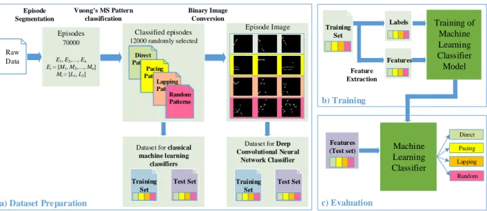
Fig. 2 illustrates a framework of the proposed MS travel pattern classifiers that consists of dataset preparation, training, and evaluation parts. In dataset preparation part, episodes (E1,
E2, …En) are segmented from the raw data which is collected
via non-invasive wireless binary sensors. Each episode consists of at least two movements (M1,M2, …Mn), and each movement
has two locations (L1 andL2). Then the segmented episodes are
classified into four patterns (direct, pacing, lapping, and
L1 L2 L3 Repetition > 2 times Locations > 2 Repetition > 1 time L4 a) Direct c) Lapping b) Pacing d) Random L1 L2 L3 L1 L2 L3 L1 L2 L3 L1 L2 L3
Fig. 1. Martino-Saltzman’s travel patterns: (a) Direct; (b) Pacing; (c) Lapping; and (d) Random. Feature Extraction Training of Machine Learning Classifier Model Machine Learning Classifier b) Training c) Evaluation Training Set Direct Pacing Lapping Random Features Labels Features (Test set) Episodes 70000 E1, E2, , En Ei = [M1, M2, , Mn] Mi = [L1, L2] Episode Segmentation Raw Data Classified episodes 12000 randomly selected Vuong s MS Pattern classification Labeled Direct Patterns Labeled Pacing Patterns Labeled Lapping Patterns Random Patterns a) Dataset Preparation Episode Image Binary Image Conversion
Dataset for classical machine learning
classifiers Training
Set
Test Set
Dataset for Deep Convolutional Neural Network Classifier Training Set Test Set `
random) according to Vuong’s [24] MS travel pattern classification algorithm. Totally 12000 episodes (3000 for each pattern) were randomly selected from over 70000 episodes for training and testing the machine learning classification models except, DCNN. For DCNN classification model, 12000 classified episodes were converted into 32×32 binary episode images as shown in Fig. 2 (a). Fig. 2 (b) illustrates the training process of the machine learning models with labels and extracted features of the training set as inputs. Fig. 2 (c) represents the evaluation part of the models where the extracted features of the test set are inputted to the trained classification model, and then the model yields the predicted labels for the corresponding features. We have used a desktop computer, which has i7-7700 CPU at 3.6 Ghz speed and NVIDIA GeForce GTX 1080 graphic card. GTX 1080 has a graphical processor unit (GPU).
A. Smart Home Environment
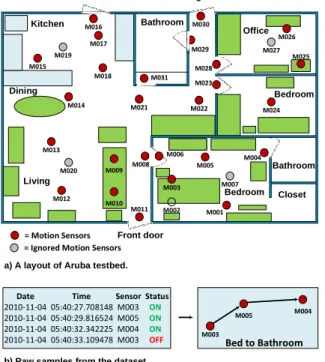
Aruba testbed, shown in Fig. 3, is one of the testbeds of CASAS project [21] that is chosen for this study. Fig. 3 (a) illustrates a layout of Aruba testbed. Aruba testbed has a kitchen, a dining area, a living room, an office, two bedrooms, two bathrooms, a pantry, a garage, and a backyard. The testbed is equipped with 31 wireless motion sensors, four door sensors, and four temperature sensors. However, only motion sensors are represented in Fig. 3 (a).
A single voluntary elderly woman lived in the Aruba testbed, and her children and grandchildren regularly visited her during the experimental period. There is no information about the resident’s exact age, cognitive state, daily activity level, etc. available in the dataset, thus we consider her as a mentally healthy person.
A. Binary Sensors
All binary sensors have a battery and a ZigBee wireless module; thus they can be installed easily on any place of the testbed and can be connected to a server via wireless mesh network. Any detected motion or no motion is an event, and events are logged chronologically in the server. Each event log consists of four parts, i.e., date, time, sensor type, and status (Fig. 3 (b)). In Fig. 3 (a), M0XX are PIR motion sensors, represented by red and grey circles that was installed on the ceiling. The red sensors sense movements under it, and the grey sensors have wider coverage area that covers most of the room. These motion sensors send a simple “ON” message when motion is present under the coverage area, followed by an “OFF” message shortly after the motion is stopped. Information of the grey sensors are ignored in this study.
B. Raw Dataset
During 625 days, 5228655 events were logged in the raw dataset from 31 PIR motion sensors, five temperature sensors, and four door switch sensors for 625. Fig. 3 (b) shows typical samples from the raw dataset. According to the samples, we realize that the resident walked from the bed to the bathroom. Supposedly, positions of the motion sensors were strategically chosen so that resident’s common visited locations are not missed.
C. Dataset Preparation
In the dataset preparation part, sensor data that was collected on days when the resident received visitors are removed from the raw dataset to separate raw dataset that belongs solely to the resident. Then, the resident’s episodes are segmented from the raw dataset using an episode segmentation algorithm as shown in Fig. 4. Furthermore, the segmented episodes classified by Vuong’s MS pattern classification algorithm were converted into four travel patterns. For DCNN, the classified episodes are converted to episode images.
1) Episode Segmentation
The dataset can be referred as one long list of consecutive movements. The episode segmentation is a process of separating the long consecutive movements into groups of movements that have spatial (start and stop location) and temporal (start and stop time) information. Episode starts when there is any movement is occurred in the testbed after the end of previous episode; and the episode stops if there is no motion for more than N seconds (N is set to 10 s in this study). Thus, a time period between the stop time of the previous movement and the start time of the consecutive movement must not exceed 10 s if those movements belong to the same episode.
Fig. 4 shows a pseudocode of an episode segmentation algorithm. The algorithm simply checks the interval time between “ON” messages of PIR sensors (line 2), and once the very first “ON” message has been received or the interval time is more than 10 s (line 4), episode index i will be incremented by one and a new episode will be created. Label of the PIR sensor will be the first location of the episode. In case of the interval time is less than 10 s, a new label different from the previous label (line 8) will be appended to the current episode.
Bathroom Closet Bedroom Front door Garage door Back door Office Living Kitchen Dining Bathroom Bedroom M010 M009 M011 M003 M002 M005 M006 M008 M007 M004 M001 M013 M014 M015 M028 M023 M024 M025 M026 M027 M019 M020 M030 M016 M017 M018 M031 M021 M022 M029 M012 = Motion Sensors = Ignored Motion Sensors
Date Time Sensor Status 2010-11-04 05:40:27.708148 M003 ON 2010-11-04 05:40:29.816524 M005 ON 2010-11-04 05:40:32.342225 M004 ON 2010-11-04 05:40:33.109478 M003 OFF M003 M005 M004 Bed to Bathroom
a) A layout of Aruba testbed.
b) Raw samples from the dataset.
Fig. 3. (a) A layout of Aruba testbed and locations of the passive infrared motion sensors; (b) Raw samples from the dataset and their representation.
2) Ground truth
We employed Vuong’s algorithm [24] to classify the segmented episodes into MS patterns, and the classified episodes are used as the ground truth for training and testing the machine learning classification models. In this study, 45000, 24000, 11000 and 3400 episodes were classified as direct, pacing, lapping, and random, respectively. Then, 12000 episodes (3000 for each pattern) were randomly chosen to form a dataset (ground truth).
3) Vuong’s MS pattern Classification Algorithm
Vuong’s algorithm determines an episode whether it belongs to the direct, pacing, lapping, or random patterns. The algorithm checks if an episode is one of the first three patterns i.e. direct, lapping and pacing. If the episode does not belong to any of these three patterns, then the episode must belong to the random pattern. First, the algorithm will check if the episode is direct, if not it will check if the episode is pacing or lapping. Finally, the episode is random if it is neither pacing nor lapping.
We explain the algorithm to check for direct, pacing, and lapping patterns. An episode is considered as direct if the episode has no repeated location or any shorter or more efficient path that connects the start and end locations. Checking for pacing pattern is done by looking for the repeated pacing sub-pattern, e.g. ‘L1L2’. For lapping patterns, we look for a pattern
(e.g., L1L2L3L1L2L3L1 or L1L2L3L1L3L2L1) which has its first
location (L1) repeated in the middle, and has at least three
different locations. Lapping can happen in the same direction and opposite direction. The detailed information of the algorithm is reported in Vuong et al. [24].
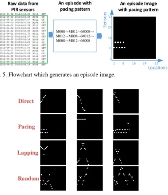
4) Episode Image
PIR motion sensors send “ON” message when they sense presence of the motion, then send “OFF” message shortly after the motion is stopped. In this study, episodes consisting of labels of 27 PIR sensors that represents the travel path of the resident. When N = 10, the longest episode has 31 movements and 32 labels. Therefore, all the episodes can be represented in a 32 × 32 binary image.
We propose a novel episode image based on binary signals of the PIR sensors. Fig. 5 shows a flowchart which generates the episode image. Suppose, a pacing episode [E = M008,
M012, M008, M012, M008, M012, M008, M012, M008] with nine locations is segmented from the raw dataset, then the segmented episode can be converted to a 32×32 binary image. In the binary image, x-axis represents the locations ranging from 1 to 32, and y-axis represents the number of PIR sensors, so the first location (M008) of the segmented episode is represented at coordinate (1, 8) by a white pixel. Since this episode has nine locations, there are nine white pixels on the episode image. Fig. 6 illustrates three sample episode images for each travel pattern.
5) Feature Extraction
Totally 8 features are extracted from each travel episode. The features are: number of movements (F1), time duration (F2), approximate distance (F3), approximate average speed (F4), entropy (F5), repeated locations (F6), repeated movements (F7), and number of pairs of opposite movements (F8). Features F5-F8 are used by Vuong et.al [24] in the machine learning classifiers for the travel pattern classification. F5 measures randomness in each episode. F6, F7, and F8 count, respectively, the occurrence of the repeated locations, the occurrence of repeated travel directions, and the occurrence of pairs of opposite travel directions in each episode. Feature F8 is needed, because a person can pace and lap in opposite directions.
To explain the mathematical derivation of the features, we assume that an episode with n locations in a chronological order is represented as a vector [24]:
𝐸 = (𝐿1, 𝐿2, … , 𝐿𝑛) (1) Algorithm 1: Episode Segmentation
Inputs: Raw PIR sensor signal sequence.
Outputs: Sequence of episodes E1, E2, …, En.
0: i = 0 # episode index 1: for all “ON” signals of PIR sensors:
2: interval= timestampnew - timestampprevious
3: timestampprevious = timestampnew
4: ifinterval > 10 s or the first “ON” signal:
5: i ++
6: Ei = [] #start a new episode list
7: Ei ← labelnew #append a new label to the list
8: else if interval < 10 s andlabelprevious ≠ labelnew:
9: Ei ← labelnew #append a new label to the list
10: end if
11: end for
Fig. 4. A pseudocode of an episode segmentation algorithm.
M008 M012 M008 M012 M008 M012 M008 M012 M008 32 1 16 1 Locations 16 32 Se n so rs 8 24 8 24 An episode Image with pacing pattern An episode with
pacing pattern Raw data from
PIR sensors
Fig. 5. Flowchart which generates an episode image.
Direct
Pacing
Lapping
Random
where 𝐿𝑖≠ 𝐿𝑖+1, 𝑖 = 1, 𝑛 − 1̅̅̅̅̅̅̅̅̅̅ and 𝐿𝑖∈ 𝐿 is a label of the
locations, L is a set of all locations. From the vector E, we find: The movements:
𝑀 = ((𝐿1, 𝐿2), (𝐿2, 𝐿3), … , (𝐿𝑛−1, 𝐿𝑛)) (2)
The set of distinct elements in vector E:
𝑆𝐸= {𝐿𝑖, 1 ≪ 𝑖 ≪ 𝑛 |𝐿𝑖∈ 𝐿} (3)
The set of distinct elements in vector M:
𝑆𝑀 = {(𝐿𝑖, 𝐿𝑖+1), 1 ≪ 𝑖 ≪ 𝑛 − 1 |(𝐿𝑖, 𝐿𝑖+1) ⊆ 𝑀} (4)
The frequency of occurrence of each element in 𝑆𝐸:
𝑓𝑖 = (number of occurrences of Liin E)/n, 1≤i≤n (5)
Then, the eight features are calculated as follows:
𝐹1 = 𝑛 − 1 (6)
𝐹2 = 𝑡𝑖𝑚𝑒𝑠𝑡𝑎𝑚𝑝𝑠𝑡𝑜𝑝− 𝑡𝑖𝑚𝑒𝑠𝑡𝑎𝑚𝑝𝑠𝑡𝑎𝑟𝑡 (7)
𝐹3 = ∑𝑛−1𝑖=1√(𝑥𝑖,2− 𝑥𝑖,1)2+ (𝑦𝑖,2− 𝑦𝑖,1)2 (8)
where 𝑥𝑖,2, 𝑥𝑖,1 are x coordinates of two locations in i-th
movement; similarly, 𝑦𝑖,2, 𝑦𝑖,1are y coordinates of two locations
in i-th movement. 𝐹4 =𝐹3 𝐹2 (9) 𝐹5 = − ∑𝑛𝑖=1𝑓𝑖𝑙𝑜𝑔𝑓𝑖 (10) 𝐹6 = 𝑛 − ‖𝑆𝐸‖ (11) 𝐹7 = 𝑛 − 1 − ‖𝑆𝑀‖ (12) 𝐹8 = ‖{1 ≤ 𝑖 ≤ 𝑛 − 1 | ∃ 𝑗, 1 ≪ 𝑖 < 𝑗 ≪ 𝑛 − 1 ∧ 𝐿𝑖= 𝐿𝑗+1∧ 𝐿𝑖+1= 𝐿𝑗}‖ (13) D. DCNN Architecture
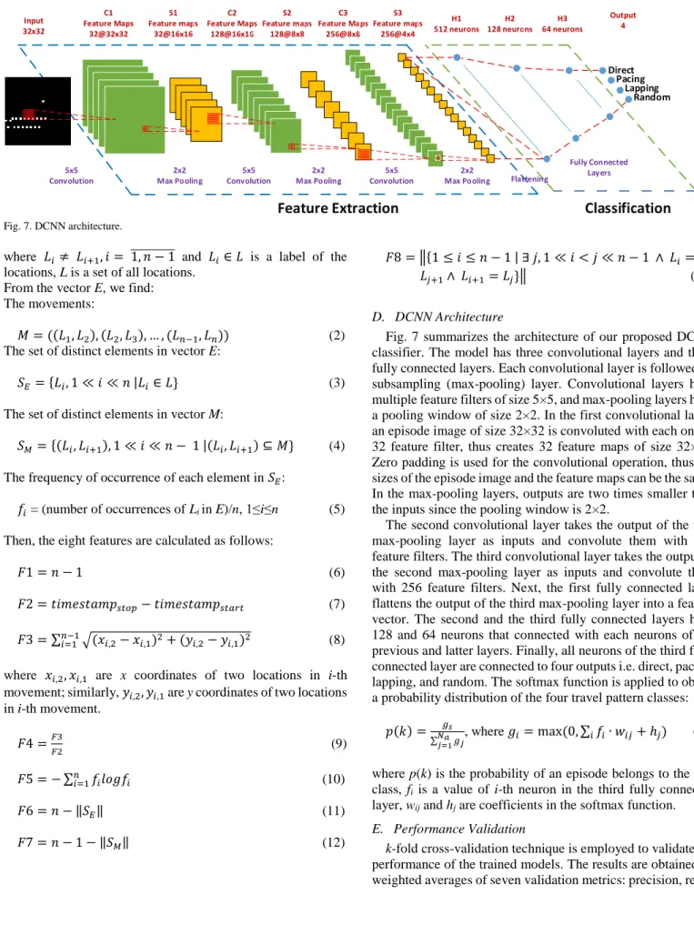
Fig. 7 summarizes the architecture of our proposed DCNN classifier. The model has three convolutional layers and three fully connected layers. Each convolutional layer is followed by subsampling (max-pooling) layer. Convolutional layers have multiple feature filters of size 5×5, and max-pooling layers have a pooling window of size 2×2. In the first convolutional layer, an episode image of size 32×32 is convoluted with each one of 32 feature filter, thus creates 32 feature maps of size 32×32. Zero padding is used for the convolutional operation, thus the sizes of the episode image and the feature maps can be the same. In the max-pooling layers, outputs are two times smaller than the inputs since the pooling window is 2×2.
The second convolutional layer takes the output of the first max-pooling layer as inputs and convolute them with 128 feature filters. The third convolutional layer takes the output of the second max-pooling layer as inputs and convolute them with 256 feature filters. Next, the first fully connected layer flattens the output of the third max-pooling layer into a feature vector. The second and the third fully connected layers have 128 and 64 neurons that connected with each neurons of the previous and latter layers. Finally, all neurons of the third fully connected layer are connected to four outputs i.e. direct, pacing, lapping, and random. The softmax function is applied to obtain a probability distribution of the four travel pattern classes:
𝑝(𝑘) = 𝑔𝑠
∑𝑁𝑎𝑗=1𝑔𝑗, where 𝑔𝑖= max (0, ∑ 𝑓𝑖 𝑖∙ 𝑤𝑖𝑗+ ℎ𝑗) (14)
where p(k) is the probability of an episode belongs to the k-th class, fi is a value of i-th neuron in the third fully connected
layer, wij and hj are coefficients in the softmax function.
E. Performance Validation
k-fold cross-validation technique is employed to validate the performance of the trained models. The results are obtained by weighted averages of seven validation metrics: precision, recall
C1 Feature Maps 32@32x32 S1 Feature maps 32@16x16 Input 32x32 5x5 Convolution 2x2 Max Pooling 5x5 Convolution 2x2 Max Pooling 5x5 Convolution 2x2 Max Pooling C2 Feature Maps 128@16x16 S2 Feature maps 128@8x8 C3 Feature Maps 256@8x8 S3 Feature maps 256@4x4 H1 512 neurons H2 128 neurons H3 64 neurons Output 4 Direct Pacing Lapping Random Flattening Fully Connected Layers
Feature Extraction
Classification
(sensitivity), specificity, F1-score, accuracy, error, and latency.
In addition, we evaluate the latency of the classifiers, which is the time period that spent for classifying an episode.
III. EXPERIMENTAL RESULTS
Table 1 represents the results of 10-fold cross-validation. For each classifier, weighted average (mean) and standard deviation of seven measures, which are averaged performances of four different patterns (direct, lapping, pacing, and random), are calculated.
NB has the poorest performance and DCNN has the highest performance. Among the four (precision, recall, specificity, and accuracy) measures, specificity is the highest for all classifiers, which reveals that all classifiers are good at avoiding false alarms. Precision is the second highest measure which is slightly higher or equal to the recall and the accuracy.
RF and GB are the second and the third highest after DCNN in terms of overall performance.
DCNN has the lowest standard deviation of 0.379%, which makes DCNN to be the best classifiers compared to the others that yields the most consistent and highest performance on all folds.
III. DISCUSSIONS
DCNN yields considerably high performance on MS travel pattern. However, the there is no annotation of travel pattern or wandering event in the dataset. Thus, we cannot detect any wandering event even that was occurred during the experimental period. However, our proposed classifier can be used for wandering detection in a real-time application.
REFERENCES
[1] N. S. Lawand et al., Sensing Technology: Current Status and Future Trends II, vol. 12. Springer, 2014.
[2] S. C. Mukhopadhyay, Next Generation Sensors and Systems, vol. 16. Springer, 2015.
[3] S. Häfner et al., “To live alone and to be depressed, an alarming combination for the renin–angiotensin–aldosterone-system (RAAS),”
Psychoneuroendocrinology, vol. 37, no. 2, pp. 230–237, Feb. 2012. [4] K. Kinsella et al., “Can populations age better, not just live longer?,”
Gener. - J. Am. Soc. Aging, vol. 37, no. 1, pp. 19–27, 2013.
[5] Worldwatch Institute, State of the World 2013: Is Sustaiability Still Possible, Island Press/Center for Resource Economics, 2013.
[6] U. S. C. Euromonitor International, “Living Alone Statistics,” 2015. [Online]. Available: http://www.statisticbrain.com/living-alone-statistics/.
[7] S. Simoens et al., “Tackling Nurse Shortages in OECD Countries,” Paris, 2005.
[8] A. Akl et al., “Autonomous unobtrusive detection of mild cognitive impairment in older adults,” IEEE Trans. Biomed. Eng., vol. 62, no. 5, pp. 1383–1394, 2015.
[9] S. Abbate et al., “MIMS: A minimally invasive monitoring sensor platform,” IEEE Sens. J., vol. 12, no. 3, pp. 677–684, 2012.
[10] N. K. Vuong et al., “Preliminary results of using inertial sensors to detect dementia-related wandering patterns,” in Proc. 37th Ann. Int. Conf. IEEE Eng. Med. Biol. Soc., 2015, pp. 3703–3706.
[11] A. Kumar et al., “A Unified Grid-based Wandering Pattern Detection Algorithm,” in Proc. 38th Ann. Int. Conf. IEEE Eng. Med. Biol. Soc., 2016, pp. 5401–5404.
[12] K.-J. Kim et al., “Dementia Wandering Detection and Activity Recognition Algorithm Using Tri-Axial Accelerometer Sensors,” in
Proc. 4th International Conference on Ubiquitous Information Technologies & Applications, 2009, pp. 1–5.
[13] K. Makimoto et al., “Japan-Korea joint project on monitoring people with dementia,” in Proc. 11th World Congress on the Internet and Med., 2006, pp. 1–5.
[14] W. D. Kearns et al., “Ultra wideband radio: A novel method for measuring wandering in persons with dementia,” Gerontechnology, vol. 7, no. 1, pp. 48–57, 2008.
[15] C. Price, “Monitoring people with dementia -- controlling or liberating?,” Qual. Ageing, vol. 8, no. 3, pp. 41–44, Apr. 2007. [16] D. Chen et al., “Intelligent video monitoring to improve safety of older
persons,” in Proc. 29th Int. Conf. IEEE Eng. in Med. and Biol. Soc., 2007, pp. 3814–3817.
[17] H. H. Dodge et al., “In-home walking speeds and variability trajectories associated with mild cognitive impairment,” Neurology, vol. 78, no. 24, pp. 1946–1952, 2012.
[18] P. N. Dawadi et al., “Automated Cognitive Health Assessment Using Smart Home Monitoring of Complex Tasks,” IEEE Trans. Syst. Man, Cybern. Syst., vol. 43, no. 6, pp. 1302–1313, Nov. 2013.
[19] B. Das et al., “One-Class Classification-Based Real-Time Activity Error Detection in Smart Homes,” IEEE J. Sel. Top. Signal Process., vol. 10, no. 5, pp. 914–923, 2016.
[20] J. Petersen et al., “Time out-of-home and cognitive, physical, and emotional wellbeing of older adults: A longitudinal mixed effects model,” PLoS One, vol. 10, no. 10, pp. 1–16, 2015.
[21] D. J. Cook, “Learning Setting-Generalized Activity Models for Smart Spaces,” IEEE Intell. Syst., vol. 27, no. 1, pp. 32–38, 2012.
[22] C. K. Y. Lai and D. G. Arthur, “Wandering behaviour in people with dementia,” J. Adv. Nurs., vol. 44, no. 2, pp. 173–182, 2003.
[23] P.-N. Wang et al., “Weight loss, nutritional status and physical activity in patients with Alzheimer’s disease. A controlled study,” J. Neurol., vol. 251, no. 3, pp. 314–20, 2004.
[24] N. K. Vuong et al., “Automated detection of wandering patterns in people with dementia,” Gerontechnology, vol. 12, no. 3, pp. 127–147, 2014.
[25] E. Batista et al., “A study on the detection of wandering patterns in human trajectories,” in Proc. 6th Int. Conf. on Information, Intelligence, Systems and Applications, 2015, pp. 1–6.
[26] D. Martino-Saltzman et al., “Travel behavior of nursing home residents perceived as wanderers and nonwanderers,” Gerontologist, vol. 31, no. 5, pp. 666–672, 1991.
TABLE I.
WEIGHTED AVERAGE AND STANDARD DEVIATION OF 10-FOLD CROSS-VALIDATION RESULTS FOR MACHINE LEARNING CLASSIFIERS.
Classifier precision recall specificity f1-score accuracy
[%] error [%] latency [ms] Naïve Bayes µ σ 0.831 0.825 0.942 0.824 82.51 17.49 < 0.02 0.01 0.011 0.004 0.011 1.14 1.14 Gradient Boost µ σ 0.943 0.941 0.98 0.941 94.06 5.94 < 0.02 0.007 0.008 0.003 0.008 0.8 0.8 Random Forest µ σ 0.947 0.945 0.982 0.945 94.48 5.52 < 0.02 0.009 0.009 0.003 0.009 0.92 0.92 DCNN µ σ 0.979 0.978 0.993 0.978 97.84 2.14 < 20 0.004 0.004 0.001 0.004 0.379 0.379