ISSN 1440-771X
Australia
Department of Econometrics
and Business Statistics
http://www.buseco.monash.edu.au/depts/ebs/pubs/wpapers/
Assessing the Impact of Market Microstructure Noise and
Random Jumps on the Relative Forecasting Performance
of Option-Implied and Returns-Based Volatility
Gael M. Martin, Andrew Reidy and Jill Wright
May 2006
Assessing the Impact of Market Microstructure Noise and
Random Jumps on the Relative Forecasting Performance of
Option-Implied and Returns-Based Volatility
Gael M. Martin, Andrew Reidy and Jill Wright
∗May 26, 2006
Abstract
This paper presents a comprehensive empirical evaluation of option-implied and returns-based forecasts of volatility, in which new developments related to the impact on measured volatility of market microstructure noise and random jumps are explicitly taken into account. The option-based component of the analysis also accommodates the concept of model-free implied volatility, such that the forecasting performance of the options market is separated from the issue of misspecification of the option pricing model. The forecasting assessment is conducted using an extensive set of observations on equity and option trades for News Corporation for the 1992 to 2001 period, yielding certain clear results. According to several different criteria, the model-free implied volatility is the best performing forecast, overall, of future volatility, with this result being robust to the way in which alternative measures of future volatility accommodate microstructure noise and jumps. Of the volatility measures considered, the one which is, in turn, best forecast by the option-implied volatility is that measure which adjusts for microstructure noise, but which retains some information about random jumps.
Keywords: Volatility Forecasts; Quadratic Variation; Intraday Volatility Measures; Model-free Implied Volatility.
JEL Classifications: C10, C53, G12.
∗Department of Econometrics and Business Statistics, Monash University. Corresponding author: Gael Martin,
Department of Econometrics and Business Statistics, P.O. Box, 11E, Monash University, Victoria, 3800, Australia. (Email: [email protected]). This research has been supported by Australian Research Council Discovery Grant No. DP0664121.
1
Introduction
In recent years, many studies have investigated the relative performance of option-implied and returns-based forecasts of the future volatility of an asset. Since the advent of the realized volatility literature (e.g. Barndorff-Neilsen and Shephard, 2002, Andersenet al.,2003), the mea-surable proxy used for the unobserved asset volatility has almost exclusively been constructed from high-frequency intraday returns. The most common such measure has been based on the sum of squared returns over small, regular intervals, such as 5 or 30 minutes (e.g. Poteshman, 2000, Blair et al.,2001, Koopman et al.,2003, Martens and Zein, 2003, Pong et al., 2004, and Jiang and Tian, 2005), with such time intervals deemed to be sufficiently small to provide an accurate estimate of volatility over the time period of interest (a day, say), whilst, at the same time, avoiding much of the bias induced by the microstructure noise present in transactions data.1 Studies that have adopted the realized volatility proxy have produced more definitive results, overall, than earlier work which used squared (or absolute) daily returns as the volatility measure (e.g. Day and Lewis, 1995). Nevertheless, conclusions have still been mixed, with the information content of option prices sometimes deemed to be superior to (or to subsume) that of historical returns (e.g. Blair et al., 2001, Jiang and Tian, 2005) and sometimes not (e.g. Martens and Zein, 2003).
The primary aim of this paper is to reassess the relative importance of option and spot prices in the prediction of future volatility by exploiting very recent developments related to the measurement of volatility in the presence of the empirical regularities of microstructure noise, including price discreteness, and random jumps. The forecasting assessments are performed using a range of measures of future volatility that are alternatives to the conventional estimator based on squared returns sampled at an arbitrarily chosen regular interval. Thefirst three such measures are designed explicitly to cater for microstructure noise, namely: the two scales realized volatility estimator of Zhanget al. (2005); the realized kernel estimator of Barndorff-Neilsenet al. (2005); and the optimal sampling frequency estimator of Bandi and Russell (2006). As a fourth alternative, we follow the approach of Anderson and Vahid (2005), by measuring only the continuous path component of future volatility, via the bi-power variation estimator of Barndorff -Neilsen and Shepherd (2004). The bi-power calculations are robustified to microstructure noise using the approach proposed in Andersen, Bollerslev and Diebold, (2005). Finally, we pursue the method of Large (2005), whereby a consistent estimator of quadratic variation, constructed from a scaled function of the discrete price movements from transaction to transaction, is based on the assumption that prices follow a pure jump process.2
1
Jiang and Tian (2005) make some adjustment to the conventional realized variance measure to accommodate autocorrelation in intraday returns; see also Andersenet al. (2003).
2
A secondary aim of our paper is to better model the efficiency of the options market by using the ‘model free’ (MF) estimate of implied volatility of Britten-Jones and Neuberger (2000) and Jiang and Tian (2005), as an alternative to the Black-Scholes (Black and Scholes, 1973) implied volatility which underlies most previous forecasting evaluations. The advantages of such an approach are two-fold. Firstly, the eschewing of a specific option price model enables a direct test of the informational content of the options market to be conducted, rather than a joint test of market efficiency and the validity of the option price model. In particular, avoidance of the empirically misspecified Black-Scholes (BS) model is likely to allow for a clearer assessment of the forecasting ability of the options market3. Secondly, as demonstrated in Jiang and Tian (2005), the particular MF volatility to be used here is an estimate of quadratic variation in the continuous and jump component of returns. Hence, in the presence of jumps in the underlying asset price process, the MF implied volatility may produce a better prediction of any measure of future volatility that itself incorporates jump information. This component of our work serves to extend the empirical analysis in Jiang and Tian (2005), in which the MF volatility measure is assessed as a predictor of one particular measure of realized volatility as constructed from regularly spaced intraday returns.
To assess the relative performance of returns- and options-based forecasts of volatility, we use both univariate and encompassing forecast regressions, in the spirit of Mincer and Zarnowitz (1969), with there being a different set of such regressions for alternative volatility proxies. All assessment is ofout-of-sample forecasting performance, with forecasts evaluated usingR2 mea-sures and various regression-based tests. Returns-based forecasts are produced bothdirectly, via time series models for the volatility proxy itself, and indirectly, via generalized autoregressive conditional heteroscedastic (GARCH)-type models for daily returns. In the spirit of much of the recent literature, and as tallies with the features of our empirical data, we focus on long memory autoregressive fractionally integrated moving average (ARFIMA) models for the volatility proxy, with short memory ARMA specifications included for comparative purposes. We also consider both short memory and long memory fractionally integrated GARCH (FIGARCH) models for daily returns, as well as certain asymmetric specifications. The forecasting assessment is con-ducted using a comprehensive set of intraday spot and option price data for News Corporation over the ten year period from 1992 to 2001.4
volatility, we expand upon the theme in Hansen and Lunde (2006a). In the latter work, the conventional realized volatility estimator, as proxy, is compared with squared daily returns, with the more accurate former measure found to produce a more reliable ranking of models in simulation experiments; see also Blairet al. (2001). Our work is also related to that of Andersen, Bollerslev, and Meddahi (2005), in which theR2 of regression-based
evaluations of alternative forecasting models are adjusted (upwards) to cater for the error-in-variables problem associated with proxying the unobserved forecast variable with a realized volatility measure that is biased in the presence of microstructure noise.
3
The BS model assumes that returns on the underlying asset are normal with constant variance; assumptions that conflict with virtually all empirical evidence onfinancial returns.
4
An outline of the remainder of the paper is as follows. In Section 2, we present the continuous time jump diffusion model for asset prices that underlies our analysis. Within the context of that model we present the conventional measure of realized volatility, based on regularly spaced returns. In Section 3, we then present the five alternative volatility proxies to be considered. The issues associated with forecasting (measured) volatility are addressed in Section 4, with the method for producing the MF implied volatility described. In Section 5, all aspects of the numerical application are outlined, including the empirical properties of the daily returns data, the option price data, the intraday data and the alternative volatility measures. Issues to do with re-scaling the latter to represent 24 hour measures are also addressed here. The results of the forecast evaluation are then presented and commented upon. Overall, the results provide quite strong evidence of the effectiveness of the MF implied volatility as a forecast of future volatility, and of the fact that the latter does best at forecasting a measure of volatility that is adjusted for microstructure noise, but which incorporates some jump information. Section 6 concludes.
2
Theoretical Model
Denoting by p(t) the logarithm of the asset price P(t) at time t, we assume a continuous time jump diffusion process,
dp(t) =µ(t)dt+σ(t)dW(t) +κ(t)dq(t), t≥0, (1) whereµ(t)is a continuous (locally bounded) function,σ(t)is a strictly positive volatility process,
W(t) is standard Brownian motion, and κ(t)dq(t) is a random jump process that allows for occasional jumps inp(t) of sizeκ(t).The quadratic variation (QV) for the return
rt+1 =p(t+ 1)−p(t) (2) is then given by QVt+1= Rt+1 t σ 2(s)ds+P t<s≤t+1κ2(s). (3)
That is, QVt+1 is equal to the sum of the integrated volatility of the continuous sample path
component (Rtt+1σ(s)ds) and the sum of theq(t)squared jumps that occur between time periods
t and t+ 1. As demonstrated in Barndorff-Neilsen and Shepherd (2002) and Andersen et al.
(2003), a consistent estimator of QVt+1 is provided by the sum of squared discretely sampled
∆-period returns, rt,∆=p(t)−p(t−∆), RVt+1(∆) =P 1/∆ j=1r 2 t+j∆,∆, (4) (www.nuff.ox.ac.uk/Users/Doornik).
whereRVt+1(∆)is referred to asrealized volatility5. That is, as ∆→0, RVt+1(∆)→ Rt+1 t σ 2(s)ds+P t<s≤t+1κ2(s). (5)
Three comments can be made about (5):
1. The result in (5) is contingent upon observed price data adhering to the model in (1). In practice, observed prices should be viewed as reflecting both the process in (1) and a process that results from market microstructure noise.
2. The sample quantityRVt+1(∆) will reflect both the continuous and jump components of
the asset price process. In particular, only in the absence of jumps (κ(t) = 0) will realized volatility estimate integrated volatility alone.
3. In practice, prices are not continuous random variables, but move in discrete numbers of ticks. This discreteness can be viewed as one component of the microstructure noise referred to in Point 1.
We take up these points in Sections 3.1, 3.2 and 3.3 respectively .
3
Alternative Approaches to Realized Volatility Calculation
3.1
Realized Volatility Calculation in the Presence of Microstructure Noise
With regard to Point 1, as highlighted in Barndorff-Neilsen et al. (2005), Zhanget al. (2005) and Bandi and Russell (2006), amongst others, observed transactions data do not adhere to (1), due to a range of factors collectively referred to as market microstructure. That is, the true price is distorted by effects that include price discreteness, separate trading prices for buyers and sellers (the bid-ask spread), the information asymmetry of market participants, and the risk aversion of market makers. Due to the presence of such factors, the ‘true’ latent logarithmic price process,p∗(t), may be assumed to follow (1), but is observed with error. Hence, a suitable model for the observed logarithmic price process,p(t), is
p(t) =p∗(t) +ε(t), (6)
whereε(t)is assumed (at least initially) to be ani.i.d.white noise component, with varianceσ2ε, and withε(t)independent ofp∗(t). Viewed in terms of the discretely sampled∆-period returns,
5As is quite common in the literature, we use the term ‘volatility’ to refer to either a variance or a standard
deviation quantity. Exactly which type of quantity is being referenced in any particular instance will be made clear by both the context and the notation.
rt,∆,we have
rt,∆ = p(t)−p(t−∆)
= p∗(t)−p∗(t−∆) +ε(t)−ε(t−∆)
= rt,∆∗ +ηt,∆. (7)
That is, observed returns (rt,∆) are equal to latent returns (r∗t,∆) plus a first order moving
average (MA) process,ηt,∆.
In practice of course, transaction data does not occur at regular time intervals, i.e. ∆between successive transactions is not constant. To reflect this fact we introduce the notation
G={t1, t2, . . . , ti, ti+1, . . . , tn}, (8)
to denote the full grid of times at which each transaction,i= 1,2, . . . , n occurs, wheren is the number of transactions in the relevant time period[t, t+ 1](i.e. on daytsay).With an obvious use of notation, the logarithmic price associated with transactionti is given by
p(ti) =p∗(ti) +ε(ti), (9)
and the observed transaction-to-transaction return expressed as
rti+1 = p(ti+1)−p(ti)
= rt∗i+1+ηti+1. (10)
Realized volatility constructed from all transactions is then defined by
RVt+1(i) = P
ti,ti+1∈[t,t+1]
r2ti+1. (11)
Beginning with the expression in (9), it is straightforward to show (see Zhang et al. 2005) that the expectation of the realized variance estimator constructed using allnof the transaction prices observed over[t, t+ 1], conditional on the true latent price process, is
E(RVt+1(i)|p∗(ti)) = P ti,ti+1∈[t,t+1]
r∗ti2+1+ 2nσ2ε. (12)
Remembering thatp∗(t) is the object assumed to follow (1), it is the quantity P
ti,ti+1∈[t,t+1]
rt∗i2+1
that estimates the quadratic variation forp∗(t), as per (4). Hence, as is clear from (12), realized volatility constructed from the observed returns is a biased representation of P
ti,ti+1∈[t,t+1]
rt∗i2+1
and, hence, a biased estimator of quadratic variation. Moreover, the bias is O(n), meaning that bias is proportional to the number of transactions used to construct the realized volatility measure. Defining c σ2 ε = 1 2nRVt+1(i), (13)
Zhanget al. (2005) also demonstrate that asn→ ∞, n1/2(cσ2
ε−σ2ε)→N(0, E(ε4)).
That is, (scaled) realized volatility constructed from observed transactions data is a consistent estimator of the variance of the microstructure noise,σ2ε!
3.1.1 The Two-Scale Realized Volatility (TSRV) Estimator
Given the clear deficiency of the realized volatility estimator based on all observed data, Zhanget al. (2005) suggest a range of modifications. Certain of these modifications bear some relationship with estimators presented in independent work of Barndorrf-Neilsenet al. (2005) and Bandi and Nelson (2006). These estimators are considered respectively in Section 3.1.2 and 3.1.3 below. We focus in this section only on the ‘first-best’ option of Zhanget al. (2005), which is based on a weighted difference between two estimators: 1) an average of realized volatilities calculated essentially as per (11), but over moving windows of subgrids defined on a ‘slow’ time scale (only observations several transactions apart are used); and 2) realized volatility calculated on a ‘fast’ time scale, as per (11) with all transactions used. More specifically, the full grid of observational points,G in (8) is partitioned intoK nonoverlapping subgrids G(k), k= 2,3, . . . , K,where
G(k)={tk−1, tk−1+K, tk−1+2K, . . . , tk−1+nkK},
for some integer nk. Realized volatility is then constructed from returns over successive time
points inG(k), denoted by ti and ti,+ respectively,
RVt(+1k)(i) = P
ti,ti,+∈G(k)
rt2i,+. (14)
The resultant two scales realized volatility (TSRV) estimator is then defined as
T SRVt+1 = µ n (K−1)nK ¶ µ RVt(+1K)(i)− nK n RVt+1(i) ¶ , (15) where RVt(+1K)(i) = 1 K K P k=2 RVt(+1k)(i), (16) RVt+1(i) is as defined in (11), nK = K1 K P k=2
nk and the scale factor,
³
n
(K−1)nK
´
, is used to improve the performance of the estimator when K is large. Clearly nK = nk if we choose a
constantnk = dim(G(k)).
The TSRV measure is shown to be a consistent estimator of quadratic variation, in the presence of microstructure noise.6 As can be deduced from the discussion in Ait-Sahalia et al.
6In Ait-Sahaliaet al. (2005) various modifications are made to the estimator in (15) to render it robust to the
presence of autocorrelated noise in (6). Given that we found little difference between these modified estimators and the estimator in (15), for the empirical data under study here, we use only the latter estimator in the forecasting evaluation.
(2005) regarding the robustness of the TSRV estimator to the deletion of outliers in the data, this estimator would be expected to eliminate some of the jump information in the data. That is, large returns impact to some extent on both the slow and fast time scale components of (15), and thereby cancel in the construction of the estimator. This is despite the fact that, theoretically, the estimator still converges to the sum of the continuous and discrete jump components of quadratic variation, as per (5).
Zhanget al. (2005) derive the optimal value for K for the periodt tot+ 1, as
K=cn2/3, (17)
wherec=¡16σ4ε/T E¡η2¢¢1/3 and η2= 43Rtt+1σ4(s)ds. The term σ4ε is square of the variance of the noise, whileRtt+1σ4(s)dsis the integrated quarticity.σ2ε is estimated as in (13) andE(η2)
estimated as E\(η2) = 4
3[RVt+1(∆)]
2 for some reasonably large ∆; see Barndorff-Neilsen et al.
(2006). In the empirical exercise we use∆≈ 30 minutes.
3.1.2 The Realized Kernel (RKERN) Estimator
Barndorff-Neilsen et al. (2005) develop kernel estimators of the quadratic variation, with the weights used in constructing the kernel chosen to ensure that the resultant estimator is consistent in the presence of microstructure noise7. Estimators that assume both regularly and irregularly
spaced data are derived. We focus here on the latter type of estimator, with returns measured in transaction time, rather than calendar time, as is consistent with the returns underlying the TSRV estimator of Zhanget al. (2005).
Consistent with the definition ofRVt(+1k)(i)in (14), (although with a slight abuse of notation), we define
RCVt(+1k)(i, h) = P
ti,ti,+,ti+h,ti+h,+∈G(k)
rti,+rti+h,+, h=−H, . . . ,−1,0,1,2, . . . H,
as the realized covariance function constructed from returns observed over pairs of successive time points in G(k),k= 2,3, . . . , K, with the returns being h time points apart.8 When h= 0, we regain the variance quantity,RVt(+1k)(i). The averaged (overk) version ofRCVt(+1k)(i, h)is then given by RCVt(+1K)(i, h) = 1 K K P k=2 RCVt(+1k)(i, h),
analogously with the averaged version ofRVt(+1k)(i),RVt(+1K)(i), in (16).
7
Although the kernel estimator is introduced within the context of general semimartingales, the properties of the estimator are demonstrated under the assumption of a model without random jumps (i.e. withκ(t) = 0in (6)).
8
The notation rti+h,+ denotes the return over successive time-points in the sub-gridG(k), where that return ishtime points distant fromrti,+ according to the sub-gridG(k), not the full gridGin (8).
A symmetric version of the realized kernel (RKERN) estimator is given by RKERNt+1 = H P h=−H whRCVt(+1K)(i, h) = w0RVt(+1K)(i) + H P h=1 wh n RCVt(+1K)(i, h) +RCVt(+1K)(i,−h)o, (18) with weights w0 = w1 = 1 (19) wh = (H+ 2h) (H−h+ 1) (H−h+ 2) H(H+ 1) (H+ 2) , h= 2,3, . . . , H. (20)
andH is the closest integer to
H= 3.6867 v u u t cσ2ε \ Rt+1 t σ2(s)ds n. (21)
The weights in (19) ensure that the kernel is asymptotically unbiased, with inclusion of the additional terms in the kernel (h= 2,3, . . . , H) serving to reduce the variance. The value of H
in (21) (approximately) minimizes the asymptotic variance of the estimator. The estimates of the noise variance (σ2ε) and integrated volatility used in the construction of H are respectively
c
σ2
ε as defined in (13) and \
Rt+1
t σ2(s)ds=RVt+1(∆),withRVt+1(∆) as defined in (4), for fairly
large∆( ∆≈30 minutes in the empirical application).
3.1.3 The Optimally Sampled Realized Volatility (OSRV) Estimator
Motivated by the relative computational simplicity of the conventional realized volatility esti-mator in (4), Bandi and Russell (2006) propose an estiesti-mator,
OSRVt+1 =PjM=1t+1rt2+jδ,δ, (22)
based onMt+1 discretely sampled δ-period returns, rt,δ = p(t)−p(t−δ),where the sampling
frequency, δt+1 = 1/Mt+1, is chosen to minimize the mean squared error (MSE). We refer to
(22) as the optimally sampled realized volatility (OSRV) estimator. Under certain conditions9, the MSE is shown to be a function ofMt+1, the second and fourth moments of the noise process,
the integrated variance,Rtt+1σ2(s)ds,and the integrated quarticity, Rtt+1σ4(s)ds.Given sample estimates of all population moments,Mt+1 is chosen so as to minimize MSE where, as indicated
by the notation, Mt+1 (and, hence, δt+1) varies with t. When the optimal sampling frequency
is high, the following approximation can be used for the optimal value ofMt+1,
Mt∗+1 ∼ Ã b Qt+1 b σ4ε !1/3 , (23) 9
where Qbt+1 = 31∆Pj1=1/∆r4t+j∆,∆, is an estimate of the integrated quarticity based upon some
relatively large time interval (∆ ≈ 30 minutes in the empirical example). The term in the denominator of (23) is given by bσ4ε = ³N M1 ∗PNt=1PMj=1∗ r2t+jδ∗,δ∗
´2
, and is an estimate of the squared second moment of the noise in (6), withδ∗ = 1/M∗equal to the highest optimal sampling frequency over theN time periods (days say) in the sample. From (23) it is clear that returns on day tare to be sampled less frequently (Mt∗+1 is smaller), the larger is the squared variance of the noise in the data relative to the quarticity of the underlying efficient price process.10
3.2
Realized Bi-Power Variation
With regard to Point 2 in Section 2, Barndorff-Neilsen and Shepherd (2004) focus on the separate identification and estimation of integrated volatility, exclusive of jumps. Defining realized bi-power variation as BP Vt+1(∆) = π 2 P1/∆ j=2|rt+j∆,∆| ¯ ¯rt+(j−1)∆,∆¯¯, (24) they show that as∆→0,
BP Vt+1(∆)
p
→Rtt+1σ(s)ds, (25)
i.e. that realized bi-power variation consistently estimates the integrated variance of the con-tinuous sample path component of the price process in (1). Using (5) and (25), it also follows that
RVt+1(∆)−BP Vt+1(∆)
p
→Pt<s≤t+1κ
2(s), (26)
with tests for jumps being based on various standardized statistics constructed from (26); see also Andersen, Bollerslev and Deibold (2005) and Huang and Tauchen (2005).
Analogous to the realized volatility estimator in (4), for very small ∆ the statistic in (25) is adversely affected by the presence of microstructure noise. Moreover, given the assumption of independent noise, the implied MA(1) structure forηt,∆ in (7) means that the two adjacent observed returns in (24) will be autocorrelated, resulting, in turn, in a source of bias in addition to that present in realized variance. To offset this bias, Andersen, Bollerslev and Deibold (2005) and Huang and Tauchen (2005) propose a modification of (24), whereby the sum of absolute adjacent returns is replaced with the sum of the corresponding one-period staggered returns, as follows BVt+1(∆) = π 2(1−2∆) −1P1/∆ j=3|rt+j∆,∆| ¯ ¯rt+(j−2)∆,∆ ¯ ¯, (27)
where the additional term in front of the sum reflects the loss of two observations due to the staggering.11 In the empirical section we implement an averaged version of (27), based on
transaction sampling,
1 0
For related work, based on the assumption of a pure jump process for the asset price, see Oomen (2006).
1 1We reserve the acronym BV for the noise-adjusted measure of bi-power variation that we use in the empirical
BVt(+1K)(i) = 1 K K P k=2 BVt(+1k)(i), (28) where BVt(+1k)(i) = 2nπn−4k P ti,ti,+,ti+2,ti+2,+∈G(k) ¯ ¯rti,+ ¯ ¯¯¯rti+2,+ ¯
¯, K is determined as per (17) above, and all subscript notation is consistent with that defined in earlier sections.
A-priori one would anticipate that direct forecasts of this measure, using historical observa-tions on it, would be more accurate than corresponding forecasts of the various realized volatility measures, which are, to some extent, influenced by the random jump component. This is the rationale underlying the forecasting exercise in Anderson and Vahid (2005). On the other hand, indirect forecasts of bi-power variation, to the extent that such forecasts themselves incorporate jump information, may be less accurate than the corresponding indirect forecasts of the realized volatility measures. These issues are investigated in Section 5.
3.3
Realized Volatility for Discrete Prices
In the spirit of Point 3 in Section 2, Large (2005) proposes an estimator of quadratic variation that focusses on the number and direction of price changes during the day, rather than the magnitude of such changes, as measured by intraday returns. The estimator, which we refer to as the ‘alternation’ estimator, is given by
ALTt+1=n(ch)tick2
C
A, (29)
where n(ch) ∈ N is the number of price changes in a day and tick is the price tick (i.e. the minimum amount by which the price can change on the relevant exchange). Defining an alterna-tion as a price change that occurs in the opposite direcalterna-tion to the previous price change, and a continuation as a price change in the same direction,A then denotes the number of alternations andC the number of continuations, withA+C=n(ch).12
Without the presence of microstructure noise, the estimatorn(ch)tick2 is a consistent
estima-tor of quadratic variation, whilst in the presence of noise the value ofn(ch)tick2 is asymptotically biased. Given that the presence of noise implies an excess of alternations, multiplication by the fractionC/A produces a consistent estimator in the presence of noise.
The modified version of the alternation estimator that we apply in the empirical investigation (see also Barndorff-Neilsen and Shephard, 2005), and which we denote by the acronym ALTM, is given by
ALT Mt+1=RVt(+1K)(i)
C
A, (30)
which is simply the (averaged) realized volatility measure in (16) multiplied byC/Ain order to correct for the upward bias induced by the noise.
1 2
4
Forecasting Volatility
4.1
Overview
Forecasts of future asset price volatility are required for various financial decisions, such as portfolio allocation, option pricing and value at risk calculation. Prior to the advent of the recent realized volatility literature, such forecasts would be produced via simple historical standard deviations (‘historical’ volatility), times series models constructed from daily returns data (e.g. GARCH-type models; exponentially weighted deterministic models such as the ‘RiskMetrics’ model; stochastic volatility models) or via implied volatilities, usually produced via the BS option pricing model. The relative worth of each competing forecast would then be measured in terms of the accuracy with which it predicted some measurable proxy for future unobserved volatility, based on low frequency (e.g. daily, weekly) returns data; see Day and Lewis (1995), amongst others.
Since the advent of the realized volatility literature, not only has the measurable proxy used for volatility changed, now being based on intraday day returns, but the focus has also shifted to the construction of standard time series models for such proxies, and the production of forecasts directly from these models. In particular, the stylized empirical properties of the (logarithmic) realized volatility measures are such that long-memory Gaussian ARFIMA models for this (transformation of) realized volatility have become the mainstay of empirical work. As such, the interest is now in the merit of these direct forecasts of some proxy of future volatility, compared with indirect forecasts based on low-frequency (usually daily) returns, in particular returns produced via the ubiquitous GARCH-type specifications. Such returns-based specifications are then compared with forecasts from the options market, with the informational efficiency of the latter thereby assessed.
In this paper, four new key questions are addressed regarding the relative performance of different volatility forecasts:
1. Which forecasting method (direct, indirect, option-implied) performs best overall when the assessment takes into account the alternative measures of volatility outlined above?
2. Is the ranking of the different forecasting methods robust to the measure of volatility used in the analysis, both as forecast variable and as the basis for the direct forecast? In other words, is the ranking robust to the different ways in which the alternative volatility measures accommodate microstructure noise and jumps?
3. Is the performance of the MF implied volatility forecast superior to that of the BS implied volatility forecast, again in the context of alternative approaches to volatility measurement?
4. What light do the results shed, if any, on the accuracy of option-based forecasts in the presence of microstructure noise, and on the way in which the options market factor in jumps?
The precise specifications of the ARFIMA and GARCH-type specifications used to produce the returns-based forecasts of volatility are determined by the properties of the data used in the empirical analysis, with discussion of those models deferred to Section 5 as a result. The way in which the option pricing model of Britten-Jones and Neuberger (2000) and Jiang and Tian (2005) model is used to produce MF implied volatility forecasts is outlined in the following section.
4.2
Model-Free Implied Volatility
A European call option is an asset that gives the owner the right to buy the underlying asset (or ‘exercise the option’) at a future point in time, T, at a pre-specified exercise or strike priceK.
The price of the option is thus dependent on the expected future price of the underlying asset which, in turn, is dependent on the assumed generating process for that underlying asset price. The BS option price model assumes that the asset price, P(t), follows a geometric Brownian motion process with constant diffusion parameter σ. In this case, the expectation that defines the BS option price has the solution,
BS(σ) =PtΦ(d1)−K−itτΦ(d2), (31) whered1 = ¡ ln(Pt/K) + ¡ it+ 0.5σ2 ¢
τ¢/σ√τ, d2 =d1 −σ√τ,Pt =the (dividend discounted)
spot price at timet,K=the strike price,it=the (annualized) risk free rate of return at timet,
τ =T−t=the time to maturity (expressed as a proportion of a year) andΦ(.) =the cumulative normal distribution. An observed market option price at timetfor a call option with maturityT
and strikeK,C(T, K), can be used to produce an estimate ofσimplied byC(T, K), by equating
C(T, K) to the right-hand-side of (31) and solving for σ. Given the joint assumptions that the BS model is valid and that the option market is efficient, the option-implied volatility estimate should subsume all information in historical volatility in terms of predicting future volatility.
As is now standard knowledge in the empirical finance literature, neither asset returns, nor market option prices adhere to the BS specifications, with stylized ‘smile’ and ‘skew’ patterns in implied volatilities across the strike price (or ‘moneyness’) spectrum being viewed as one manifestation of the misspecification of the model. Despite the large amount of attention devoted to producing alternative option price formulae that cater for the standard empirical features of asset returns (e.g. Heston, 1993, Bakshiet al.,1997, Corrado and Su, 1997, Bates, 2000, Heston and Nandi, 2000, Limet al., 2005), it is the BS option formula that still underlies the implied
volatilities used in many assessments of the relative performance of option-implied and returns-based volatility forecasts. As a consequence, it could be argued that these results are subject to model misspecification errors, and do not necessarily give a clear indication of the quality of information present in the options market.
With this misspecification issue in mind, we adopt the MF approach to implied volatility calculation of Britten-Jones and Neubeger (2000) and Jiang and Tian (2005). As demonstrated by these authors, under the assumption of a diffusion process for the spot price, P(t), a (risk-neutral) forecast of integrated variance for the periodt to T can be determined from observed call option prices with maturityT as follows
Et " T R t σ2(s)ds # = 2∞R 0 Ct(T, K)eitτ−max £ 0, Pteitτ−K ¤ K2 dK, (32)
where all notation is as defined above. The calculation in (32) invokes no specific assumptions about the spot price process. Given afinite number of strike prices, with maximum and minimum valuesKmax and Kmin respectively, (32) is estimated as
Et " T R t σ2(s)ds # ≈ 2 KmaxR Kmin Ct(T, K)eit(T−t)−max £ 0, Pteit(T−t)−K ¤ K2 dK ≈ M P j=1 [g(T, Kj) +g(T, Kj−1)]∆K, (33)
where∆K= (Kmax−Kmin)/M,Kj =Kmin+j∆Kfor0≤j≤Mandg(T, Kj) = (Ct(T, Kj)eit(T−t)
−max£0, Pteit(T−t)−Kj
¤
)/K2
j.Given the limited number of strikes (and hence option prices)
that occur in any empirical setting, a curve-fitting method is used to interpolate between the observed strikes. The procedure adopted follows that of Jiang and Tian (2005), with steps as follows: 1) Use observed call option prices (for available strikes) to produce implied BS volatili-ties, via (31); 2) Fit a smooth function to the implied volatilities and use this function to extract implied volatilities at grid pointsKj;3) Use the BS model in (31) to translate theKj into
‘ob-served’ pricesCt(T, Kj);4) Use the full set ofM Kj andCt(T, Kj)values to estimate integrated
volatility as in (33).13 The implied volatility extracted from option prices observed at time t,
Ct(T, Kj), represents the market’s estimate of volatility over the maturity periodttoT.14 In the
forecasting exercise, in order to avoid to so-called ‘telescoping’ problem (see Christensen et al.,
2001) we artificially construct options that always have an expiry of approximately 22 trading
1 3
As pointed out by Jiang and Tian (2005), the BS model is simply being used as a mechanism to produce (artificially) a larger range of strike prices than is available in practice. The curvefitting procedure followed here does not require the BS model to be the ‘true’ model underlying the observed prices.
1 4Following Jiang and Tian (2005) we do not use options which expire within one week. We also only use
observed prices of options with a moneyness between 0.9 and 1.1. The moneyness of an option is a function of the difference between the strike price and the spot price at timet.Broadly, options are said to be out-of-the-money ifPt< K, in-the-money ifPt> K and at-(or near-) the-money ifPt≈K.
days ahead.15
As demonstrated in Jiang and Tian (2005), the result in (32) can be extended to jump-diffusion processes, in which case the method produces a forecast of quadratic variation. That is, in the case where the true latent price follows the model in (1), the implied variance is an estimate of (3), rather than an estimate of integrated volatility only.
5
Empirical Analysis Using Australian Stock Market Data
5.1
Introduction
The numerical analysis is performed using data on equity and option trades for the Australian listed company, News Corporation (Newscorp) over the ten year period from 2 January, 1992 to 28 December 2001.16 Rolling one step ahead forecasts are produced for the period 9 January, 1997 to 28 December 2001, meaning that the one step ahead forecast regressions are estimated using 1249 observations. Ten and 22 steps ahead forecasts are produced over the same period, with the associated forecast regressions based on 1239 and 1227 observations respectively. Each returns-based forecast is produced using both daily and intraday observations fromN = 1000
days. Thefirst year of observations (2 January to 30 December, 1992) is used to set pre-sample values in the estimation of the long-memory models. Each option-implied forecast is based on option prices observed on the day immediately prior to the forecast day (or period).
In Section 5.2 we present a brief descriptive analysis of all relevant empirical features of the data (both equity and option data), followed by a documentation of the key empirical features of the alternative volatility measures in Section 5.3. Section 5.4 then reports all results regarding the evaluation of those alternative forecasts, with the key research questions outlined earlier addressed.
1 5
To do this we take the set of options that are the closest and second closest to expiry. For example the closest expiry date may bet+ 18, while the second closest may bet+ 40.In step 1) above, the BS implied volatilites are calculated for all options expiring ont+ 18(with moneyness between 0.9 and 1.1). A parabola is thenfitted to these BS implied volatilities as per step 2). The same two steps are performed for the set of options expiring on
t+ 40.These two BS implied volatility curves are then linearly interpolated between to obtain a implied volatility curve for dayt+ 22.Outside of the moneyness interval, 0.9 to 1.1, we construct extrapolated call prices using the BS model with an implied volatility set equal to the implied volatility at moneyness of 0.9 or 1.1 depending on which is the closest.
1 6Newscorp is one of the world’s largest media conglomerates with USD $23.859 billion in revenue in 2005.
In Australia, Newscorp owns 17 newspapers, however most of its assets are located overseas with the most well known being the Fox Broadcasting Corporation. In 2004, Newscorp was re-incorporated in the US. It now trades on the New York Stock Exchange, the London Stock Exchange and the ASX.
5.2
Empirical Features
5.2.1 Daily Returns Data
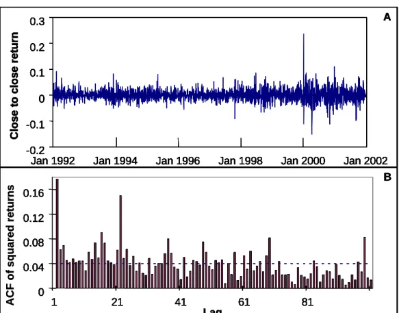
Panel A of Figure 1 shows the daily (close to close) returns over the 1992 to 2001 period, adjusted for share splits and dividends, andfiltered as described in Appendix A.17 The kurtosis, skewness and Jarque-Bera statistics are respectively 11.224, 0.467 and 7150.730, indicating significant excess kurtosis and (positive) skewness, using 5% asymptotic critical values. Panel B of Figure 1 is the autocorrelation function (ACF) of squared daily returns, which is a proxy for daily volatility. The dotted line in the figure is the asymptotic upper 95% confidence bound. As is typical for squared returns, the ACF decays relatively slowly, with significant correlation remaining after 80 lags.
-0.2 -0.1 0 0.1 0.2 0.3
Jan 1992 Jan 1994 Jan 1996 Jan 1998 Jan 2000 Jan 2002
C lose t o c lose r e tu rn A 0 0.04 0.08 0.12 0.16 1 21 41 61 81 Lag B -0.2 -0.1 0 0.1 0.2 0.3
Jan 1992 Jan 1994 Jan 1996 Jan 1998 Jan 2000 Jan 2002
C lose t o c lose r e tu rn A -0.2 -0.1 0 0.1 0.2 0.3
Jan 1992 Jan 1994 Jan 1996 Jan 1998 Jan 2000 Jan 2002
C lose t o c lose r e tu rn A 0 0.04 0.08 0.12 0.16 1 21 41 61 81 Lag B 0 0.04 0.08 0.12 0.16 1 21 41 61 81 Lag A C F o f s quar e d ret urns B -0.2 -0.1 0 0.1 0.2 0.3
Jan 1992 Jan 1994 Jan 1996 Jan 1998 Jan 2000 Jan 2002
C lose t o c lose r e tu rn A -0.2 -0.1 0 0.1 0.2 0.3
Jan 1992 Jan 1994 Jan 1996 Jan 1998 Jan 2000 Jan 2002
C lose t o c lose r e tu rn A 0 0.04 0.08 0.12 0.16 1 21 41 61 81 Lag B -0.2 -0.1 0 0.1 0.2 0.3
Jan 1992 Jan 1994 Jan 1996 Jan 1998 Jan 2000 Jan 2002
C lose t o c lose r e tu rn A -0.2 -0.1 0 0.1 0.2 0.3
Jan 1992 Jan 1994 Jan 1996 Jan 1998 Jan 2000 Jan 2002
C lose t o c lose r e tu rn A 0 0.04 0.08 0.12 0.16 1 21 41 61 81 Lag B 0 0.04 0.08 0.12 0.16 1 21 41 61 81 Lag A C F o f s quar e d ret urns B
Figure 1: Panel A: close to close daily returns for Newscorp over the period 2 January 1992 to 28 December 2001. Panel B: autocorrelation function (ACF) of squared daily returns over this period. The dotted line is the upper 95% confidence bound.
In order to cater for the empirical features of the daily returns data, preliminary analysis
1 7The largest one day increase in the share price occurs on 11 January 2000, at the time of the merger of America
Online and Time Warner (Collins, 2000a). The largest one day decrease occurs on 17 April 2000, associated with a large decrease on the NASDAQ market (Collins 2000b).
focussed on a range of GARCH-type specifications with leptokurtic conditional distributions. Givenrt+1 =µ+εt+1 =µ+σt+1et+1, where rt+1 denotes the daily return in (2),µ the mean
daily return,σ2t+1 the daily variance andet+1∼Student t(0,1, ν), model selection criteria and
significance tests were used to choose the following GARCH, threshold GARCH (TGARCH), asymmetric power ARCH (APARCH)) and fractionally integrated GARCH (FIGARCH)) mod-els for use in the forecasting exercise:
GARCH(1,1) : σ2t+1 =ω+αε2t +βσ2t
T GARCH(1,1) : σ2t+1 =ω+αεt2+αγst+1ε2t +βσ2t (34)
AP ARCH(1,1) : σδt+1 =ω+α|εt|δ−αγ∗st+1|εt|δ+βσδt
F IGARCH(1, d,1) : (1−L)d(1−αL)ε2t+1 =ω+ (1−βL)σ2t+1.
The notationLis used to denote the lag operator,d >−1is the fractional parameter,(1−L)d= P∞
j=0bjLj,with b0 = 1and bj = Γ(1−−dΓd()jΓ−(jd+1)) , and the remaining parameters satisfy the usual
restrictions. In the asymmetric models (TGARCH and APARCH) st+1 = 1 if εt < 0 and 0
otherwise, with the APARCH model nesting the TGARCH model when γ∗=−γand δ = 2.
All models are estimated using conditional maximum likelihood, with the infinite lag struc-ture in the FIGARCH model truncated at the lag determined by the number of sample obser-vations plus the number of pre-sample obserobser-vations. For the rolling samples, the persistence of the GARCH model (α+β) varies from 0.820 and 0.997 and the degrees of freedom for the conditional Student t distribution (ν) varies from 4.9 to 12, with similar results for the other models. In the FIGARCH model the long memory parameter (d) varies from 0.09 to 0.39 over the rolling period. For the asymmetric models (TGARCH and APARCH), the estimate of the asymmetry parameters(γ and γ∗)are found to be insignificant at the 5% level during the model
selection period (1993-1996), but significant for some of the rolling samples used to produce the forecasts, ranging from about 0.1 to 2 (in magnitude).
5.2.2 Option Price Data
Options transaction data for Newscorp were obtained from the ASX for the period 8 January 1997 to 27 December 2001. The forecasting analysis is based only on transactions that occur within the last hour of trading (3pm to 4pm) for each trading day during this period. In this way, the implied volatility estimates produced from the option price data can be viewed as a forecast of volatility over the next day(s). The average number of option prices used in the calculation of implied volatility estimates on each day is 38.
As the spot market for Newscorp stock is very liquid, for each option trade it is possible to obtain a virtually simultaneous equity price: usually recorded within a few seconds of the option trade. When several equity trades are recorded at exactly the same time, a weighted
average is taken, with the weights determined by the trading volume. With reference to the option price formulae in (31) and (33), it is equated to the three month bond rate on day t.18
The dividends paid on Newscorp shares average about 0.1% of share value, and are paid six-monthly. The impact of dividends on share prices is therefore so small that they have only been taken into account as a constant continuous discount factor, with Pt in (31) and (33) replaced
byPte−d(T−t), where dis the average dividend rate over the sample period.19
0 0.2 0.4 0.6 0.8 1
Jan-1997 Jan-1998 Jan-1999 Jan-2000 Jan-2001
B 0 0.2 0.4 0.6 0.8
Jan 1997 Jan 1998 Jan 1999 Jan 2000 Jan 2001
Impli e d Vo la tilit y Black Scholes Model free A 0 0.2 0.4 0.6 0.8 1
Jan-1997 Jan-1998 Jan-1999 Jan-2000 Jan-2001
B 0 0.2 0.4 0.6 0.8
Jan 1997 Jan 1998 Jan 1999 Jan 2000 Jan 2001
Impli e d Vo la tilit y Black Scholes Model free A
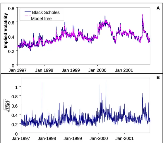
Figure 2: Panel A: one step ahead (annualized) implied volatility forecasts for the period 8 January 1997 to 27 December 2001 calculated using the BS and MF specifications. Panel B: next day (annualized)√T SRV calculated over this period.
Implied volatility estimates are produced via both the MF approach described in Section 4.2 and the BS model, (31), for the purpose of comparison. We adopt an approach to BS implied volatility calculation that is fairly representative of that adopted by others. That is, four
close-1 8The interest rate data has been obtained from the Reserve Bank of Australia website: www.rba.gov.au. 1 9
As are most stock options traded on the ASX, Newscorp (NCP) options are American options. However, as noted, dividends paid on this particular stock are infrequent and negligible in magnitude. In this case, the European formulae used to produce the implied volatility estimates, with the current spot price discounted as described in the text, are appropriate; see Hull (2000).
to-the-money options (one put and one call above and below the money) with maturity as close as possible to the forecast horizon (but with at least one week to maturity), are selected from the last hour of trading for each day.20 The implied volatility is then calculated by minimizing the sum of squared percentage deviations of the observed prices from the BS option price in (31).21
Panel A of Figure 2 shows the one step ahead (annualized) implied volatility forecasts cal-culated over 8 January 1997 to 27 December 2001 using both option specifications. Both series track each other fairly closely, but with the MF volatility series being slightly smoother than the BS series. This extra smoothness is perhaps to be expected, given the extra degree of averaging (across both strikes and maturities) that occurs in the computation of the MF volatility. Pre-empting the forecasting assessment in Section 5.4 we show in Panel B the next-day volatility, calculated using the TSRV measure in (15). The measure is re-weighted in the manner to be described in Section 5.3.4, then presented in annualized standard deviation form. It can be seen that both implied volatility predictions track the√T SRV series closely, with the implied volatil-ity series much smoother because they represent the market’s forecasts of volatilvolatil-ity over longer time horizons than one day. Note also that both implied volatility series are biased upward as forecasts of the next-day√T SRV measure, which is expected due to the implicit risk premium factored into option prices; see, for example, Guo (1998).
5.2.3 Intraday Data
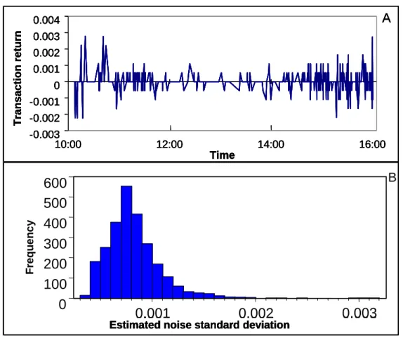
The realized volatility and bi-power measures are constructed using the prices of all intraday transactions, including successive transactions for which there is no price change.22 Panel A of Figure 3 plots the transaction-to-transaction returns for Newscorp for 1 August 2001 from 10am to 4pm. According to the model in (10), the observed return is a sum of the return in the latent price process and the noise process, where the latter has variance estimated consistently by the estimator in (13). It can be seen that there are many small returns which would be noise induced by the bid-ask bounce alone. Panel B of Figure 3 is a histogram showing the estimate of the standard deviation of the noise, as calculated using (13), for the period 2 January 1992 to 28 December 2001. The magnitude of these numbers indicates that the transaction data contains a substantial amount of noise that needs to be accounted for when estimating the volatility of the efficient price. Over the sample period, the noise to signal ratio, estimated as
2 0
When more than one option satifies the criteria for a particular option category, the option which is both traded closest to 4pm and closest to the money is selected.
2 1
As noted in Section 4.2, the MF implied volatilities do not suffer fom the so-called ‘telescoping’ problem, whereby the maturity with which the implied volatility forecast is associated changes witht.The BS forecasts will suffer from this problem to some extent.
2 2
The only exception to this is in the calculation of the noise variance estimates, in which case we use only only non-zero transactions (referred to as ‘tick’ sampling by Griffin and Oomen, 2006).
q c
σ2
ε/
√
T SRV, decays consistently from approximately 0.15 in 1992 to approximately 0.04 in 200123. These figures correspond respectively to the ‘large noise’ and ‘moderate noise’ cases in
Barndorff-Neilsenet al. (2005). The mean value of
q c
σ2
ε, 0.0008, is also very similar to the mean
value of the corresponding noise estimate for the S&P100 over one month in 2002, 0.0007, as reported in Bandi and Russel (2006).
0
100
200
300
400
500
600
0.001
0.002
0.003
0
100
200
300
400
500
600
0.001
0.002
0.003
0
100
200
300
400
500
600
0.001
0.002
0.003
0
100
200
300
400
500
600
0.001
0.002
0.003
-0.003 -0.002 -0.001 0 0.001 0.002 0.003 0.004 10:00 12:00 14:00 16:00 Time Trans action returnA
Estimated noise standard deviation
B
0
100
200
300
400
500
600
0.001
0.002
0.003
0
100
200
300
400
500
600
0.001
0.002
0.003
0
100
200
300
400
500
600
0.001
0.002
0.003
0
100
200
300
400
500
600
0.001
0.002
0.003
0
100
200
300
400
500
600
0.001
0.002
0.003
0
100
200
300
400
500
600
0.001
0.002
0.003
0
100
200
300
400
500
600
0.001
0.002
0.003
0
100
200
300
400
500
600
0.001
0.002
0.003
-0.003 -0.002 -0.001 0 0.001 0.002 0.003 0.004 10:00 12:00 14:00 16:00 Time Trans action returnA
Estimated noise standard deviation
B
F re q ue nc y0
100
200
300
400
500
600
0.001
0.002
0.003
0
100
200
300
400
500
600
0.001
0.002
0.003
0
100
200
300
400
500
600
0.001
0.002
0.003
0
100
200
300
400
500
600
0.001
0.002
0.003
0
100
200
300
400
500
600
0.001
0.002
0.003
0
100
200
300
400
500
600
0.001
0.002
0.003
0
100
200
300
400
500
600
0.001
0.002
0.003
0
100
200
300
400
500
600
0.001
0.002
0.003
-0.003 -0.002 -0.001 0 0.001 0.002 0.003 0.004 10:00 12:00 14:00 16:00 Time Trans action returnA
Estimated noise standard deviation
B
0
100
200
300
400
500
600
0.001
0.002
0.003
0
100
200
300
400
500
600
0.001
0.002
0.003
0
100
200
300
400
500
600
0.001
0.002
0.003
0
100
200
300
400
500
600
0.001
0.002
0.003
0
100
200
300
400
500
600
0.001
0.002
0.003
0
100
200
300
400
500
600
0.001
0.002
0.003
0
100
200
300
400
500
600
0.001
0.002
0.003
0
100
200
300
400
500
600
0.001
0.002
0.003
-0.003 -0.002 -0.001 0 0.001 0.002 0.003 0.004 10:00 12:00 14:00 16:00 Time Trans action returnA
Estimated noise standard deviation
B
F re q ue nc yFigure 3: Panel A: intraday transaction to transaction return for 1 August 2001 from 10am to 4pm. Panel B: histogram of the estimated standard deviation of the noise
µq c
σ2
ε
for each day over the period 2 January 1992 to 28 December 2001.
5.3
Alternative Volatility Measures
5.3.1 Signature Plots
Signature plots graph realized volatility and bi-power measures across a range of different sam-pling frequencies; see, for example, Andersen et al. (2000). At each sampling frequency, the variance measure is an average of the measure calculated at that frequency, on each day in the
2 3
This decline is in part due to the much higher liquidity in the later part of the sample, which causes, in turn, a reduction in the bid-ask spread.
sample. Signature plots provide a way of visualizing bias problems with realized volatility and bi-power measures. An estimator that is robust to microstructure noise should produce an ap-proximatelyflat signature plot. Although the focus of our analysis in on predictive performance, robustness according to the signature plots remains an important consideration.
0 0 . 0 0 4 0 . 0 0 8 0 . 0 1 2 0 5 1 0 1 5 2 0 2 5 3 0 S a m p l i n g F r e q u e n c y ( , m i n u t e s ) Mean Vo latilit y R a w R V I n t e r p o l a t e d R V A 0 0 . 0 0 4 0 . 0 0 8 0 . 0 1 2 0 . 0 1 6 0 1 0 2 0 3 0 4 0 5 0 T r a n s a c t i o n S a m p l i n g F r e q u e n c y ( K ) Mean Vo la tilit y T S R V R K E R N A L T B V B 0 0 . 0 0 4 0 . 0 0 8 0 . 0 1 2 0 5 1 0 1 5 2 0 2 5 3 0 S a m p l i n g F r e q u e n c y ( , m i n u t e s ) Mean Vo latilit y R a w R V I n t e r p o l a t e d R V A 0 0 . 0 0 4 0 . 0 0 8 0 . 0 1 2 0 5 1 0 1 5 2 0 2 5 3 0 S a m p l i n g F r e q u e n c y ( , m i n u t e s ) Mean Vo latilit y R a w R V I n t e r p o l a t e d R V A 0 0 . 0 0 4 0 . 0 0 8 0 . 0 1 2 0 . 0 1 6 0 1 0 2 0 3 0 4 0 5 0 T r a n s a c t i o n S a m p l i n g F r e q u e n c y ( K ) Mean Vo la tilit y T S R V R K E R N A L T B V B
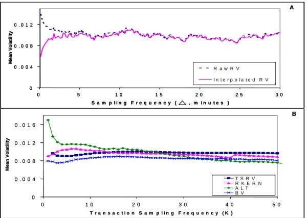
Figure 4: Panel A: Signature plots of Raw RV(∆) and Interpolated RV(∆) against ∆. The series shown are averaged over the trading days in August 2001. The average optimal sampling frequency over this period, calculated via (23), is 5.36 minutes. Panel B: signature plots of TSRV, RKERN, ALTM and BV againstK.The series shown are averaged over the trading days in August 2001. The average optimal sampling frequency over this period, calculated as (17) is
K= 3.
Panel A in Figure 4 plots two versions of RV(∆) in (4) over different time periods ∆.Given that the observed data is irregularly spaced, two main choices are available for construction of RV(∆) at regularly spaced points in time determined by∆.With the so-called “raw” sampling method, if a transaction price is not observed at a given time point, then the previous transaction price is used as the sampled price. With the “linear interpolation” method, if a price is not observed at a given time point, then the sampled price is obtained by linearly interpolating between the price of the previous and next transaction. As∆→0, raw sampling produces an estimator that mimics the behaviour of the transaction based RV estimator in (11) asn→ ∞;
Figure 4. As noted by Hansen and Lunde (2006b), the linear interpolation method can produce downward bias at high frequencies, as is also evident in Panel A. Clearly there is little to choose between the two methods for ∆ = 5 minutes onwards. In the empirical application we use the linear interpolation method in constructing RV(5), RV(15) and OSRV, with the optimal frequency used in the construction of OSRV varying between approximately 5 and 30 minutes across the sample period.
In Panel B of Figure 4 we plot the four transactions-based estimators: TSRV in (15), RKERN in (18), ALTM in (30) and BV in (28), against sampling frequencyK.24 Four features are worthy
of note. Firstly, the ALTM performance is the worst, with the value of the estimator changing substantially as K declines.25 Secondly, the other three estimators have very similar, and very
flat signature plots, meaning that the nature of their construction has served to render them quite robust to the microstructure noise that contaminates the RV(∆) measures at high frequencies. Thirdly, all four signature plots are smoother than those in Panel A due, in the main, to the averaging acrossk(k= 2,3, . . . , K) used in the construction of the measures. Finally, the TSRV estimator has theflattest signature plot of all those considered.
5.3.2 Disributional and Memory Properties
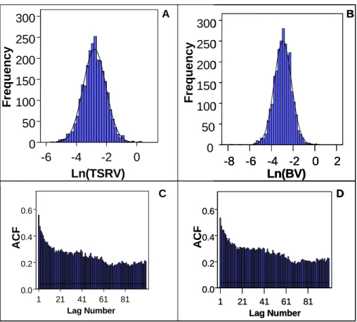
Panels A and B of Figure 5 display histograms of the natural logarithms of the TSRV and BV volatility measures, and panels C and D the ACF’s for the two measures. The corresponding results for the other measures are qualitatively similar and, hence, not reported. The normal densities imposed on the empirical densities demonstrate that the log of the variance measures are well approximated by a normal distribution, but with a small amount of excess kurtosis evident. The slow decline in the ACF’s is typical of the memory behaviour exhibited throughout the literature for intraday data-based volatility measures; see, for example Andersenet al. (2003).
To cater for these empirical features, we produce direct forecasts using the following
ARFIMA(p,d,q) model with Student t innovations (where the generic notationyt refers to the
logarithm of any of the volatility measures described in Section 3, and αits mean):
φ(L)(1−L)d(lnyt−α) =θ(L)ut ; ut∼Student t (0, σ2
ν ν−2, ν).
The autoregressive and moving average polynomials φ(L) and θ(L) are of lag length p and q
respectively and(1−L)dis as defined earlier. The ARFIMA (p,d,q) models are estimated using conditional maximum likelihood, with the infinite lag structure induced by(1−L)dtruncated at
2 4
Note that in the empirical exercise, the optimal value of K in (17) varies between approximately 2 and 6 across the sample period.
2 5ALTM is based on the assumption that quoted prices change by the minimum tick value ($0.01 in our case).
While this assumption may be valid for very actively traded stocks on large exchanges, wefind that for our data the price change is commonly ten times the minimum tick amount. This may be a reason why ALTM does not perform as well as the other measures according to the signature plots.
81 61 41 21 1 Lag Number 0.6 0.4 0.2 0.0 81 61 41 21 1 Lag Number 0.6 0.4 0.2 0.0 ACF 0 -2 -4 -6 Ln(TSRV) 300 250 200 150 100 50 0 Fr eq u e ncy A 2 0 -2 -4 -6 -8 Ln(BV) 300 250 200 150 100 50 0 Fr eq ue ncy B D C ACF 81 61 41 21 1 Lag Number 0.6 0.4 0.2 0.0 81 61 41 21 1 Lag Number 0.6 0.4 0.2 0.0 ACF 0 -2 -4 -6 Ln(TSRV) 300 250 200 150 100 50 0 Fr eq u e ncy A 2 0 -2 -4 -6 -8 Ln(BV) 300 250 200 150 100 50 0 Fr eq ue ncy B D C 81 61 41 21 1 Lag Number 0.6 0.4 0.2 0.0 ACF 81 61 41 21 1 Lag Number 0.6 0.4 0.2 0.0 ACF 0 -2 -4 -6 Ln(TSRV) 300 250 200 150 100 50 0 Fr eq u e ncy A 2 0 -2 -4 -6 -8 Ln(BV) 300 250 200 150 100 50 0 Fr eq ue ncy B D C ACF
Figure 5: Panel A and B: histogram, with normal density superimposed, of ln(TSRV) and ln(BV) respectively (24 hour weighted and annualized) for the period 2 January 1992 to 28 December 2001. Panel C and D: autocorrelation function (ACF) for each measure over the same period.
the lag determined by the number of sample observations plus the number of pre-sample obser-vations. Preliminary analysis has led to the use of ARFIMA (0,d,1) specifications in producing all forecasts. The rolling estimates ofdrange from0.27to0.36, values which are typical for this type of data; see, for example, Andersen et al. (2003). For comparative purposes we also pro-duce forecasts via short memory ARMA (2,0,1) models, with the lag lengths again determined via preliminary analysis.26
5.3.3 The Impact of Jumps
Of all alternatives considered, the two measures expected to display less volatile behaviour, due to their handling of jumps, are the BV and TSRV measures. As described in Section 3.2, the former measure is explicitly designed to estimate only the continuous component of quadratic variation. The latter measure, on the other hand, is expected to incorporate less jump
2 6
Note that the application of standard model selection criteria to both ARFIMA and ARMA models for the different measures lead to slightly different choices ofpandq.It was decided to use just one specification (of each model) for all measures.
information due to the nature of its construction, despite the fact that it formally converges to the sum of the continuous and jump components of quadratic variation, as per the results in Zhanget al. (2005).
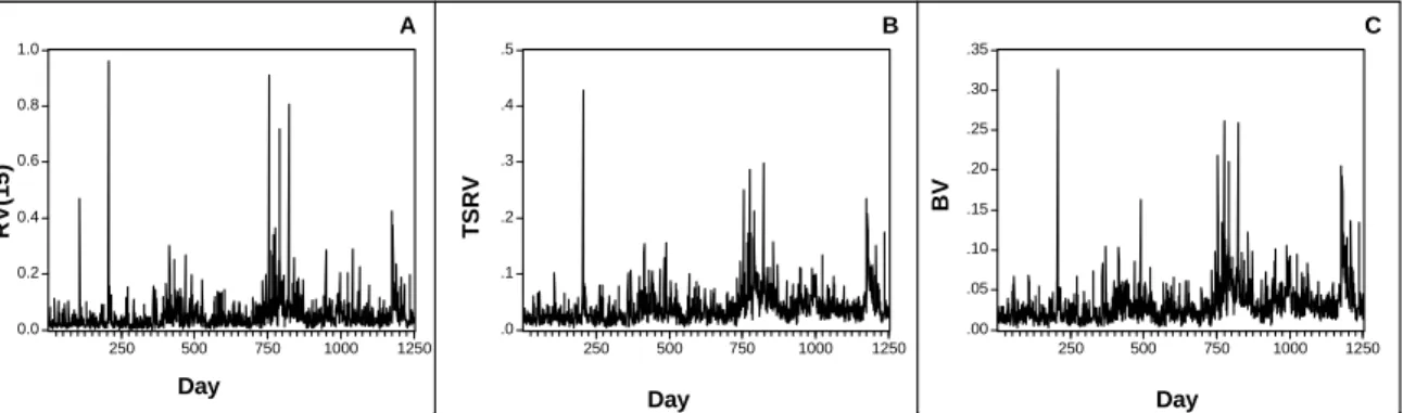
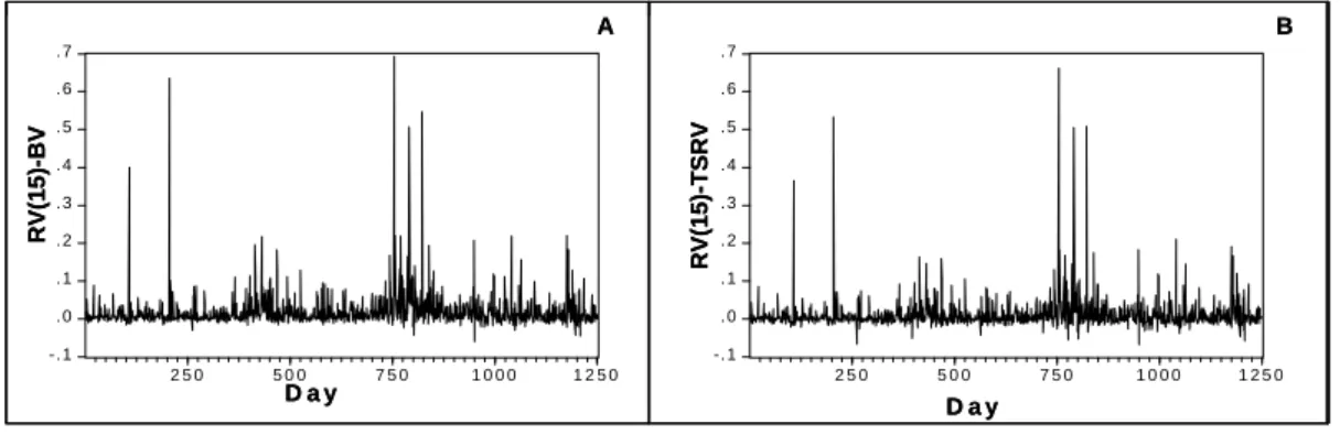
In Figure 6, Panels A, B, and C respectively, we plot the time series of RV(15), TSRV, and BV over the time period used in the forecasting evaluation in Section 5.4. RV(15) is included as an estimate of quadratic variation, BV as estimate of the continuous component of quadratic variation, and TSRV as an estimator of quadratic variation in which the impact of jump variation is nonetheless reduced. In Figure 7, Panels A and B we then plot the difference between RV(15) and each of the two alternative estimators. As expected, BV displays less volatile behaviour than TSRV. The difference between RV(15) and BV in Panel A is formally an estimate of the jump component of quadratic variation. The graph in Panel B is an indication of the extent of jump behaviour that remains after the construction of the TSRV estimator via the difference in (15). As would be expected, the latter does not eliminate jump variation to the same extent as does BV, a fact which accords with the plots in Panels B and C of Figure 6. A priori, we would expect the relative smoothness of the alternative volatility series to have an impact on their forecasting performance, and on their ability to be forecast. This expectation is indeed vindicated by the empirical results in Section 5.4.
0.0 0.2 0.4 0.6 0.8 1.0 250 500 750 1000 1250 .0 .1 .2 .3 .4 .5 250 500 750 1000 1250 .00 .05 .10 .15 .20 .25 .30 .35 250 500 750 1000 1250 RV (1 5) TS RV BV Day Day Day A B C 0.0 0.2 0.4 0.6 0.8 1.0 250 500 750 1000 1250 .0 .1 .2 .3 .4 .5 250 500 750 1000 1250 .00 .05 .10 .15 .20 .25 .30 .35 250 500 750 1000 1250 RV (1 5) TS RV BV Day Day Day A B C
Figure 6: Panels A, B and C plot respectively the RV(15), TSRV and BV series for the January, 1997 to December 2001 period over which the forecast evaluation is performed.
5.3.4 Variance Measures for the Whole Day
Due to the fact that the ASX is open only for several hours during the trading day, the realized volatility and bi-power measures do not contain that portion of daily (i.e. 24 hour) volatility that is associated with the overnight return. Given that the overnight return, in this case, reflects price activity in the major U.S, U.K. and European exchanges, volatility in this component of the daily return may well be a significant component of the overall volatility for the 24 hour period.
-. 1 . 0 . 1 . 2 . 3 . 4 . 5 . 6 . 7 2 5 0 5 0 0 7 5 0 1 0 0 0 1 2 5 0 -. 1 . 0 . 1 . 2 . 3 . 4 . 5 . 6 . 7 2 5 0 5 0 0 7 5 0 1 0 0 0 1 2 5 0 RV (1 5) -B V RV(15) -TSRV D a y D a y A B -. 1 . 0 . 1 . 2 . 3 . 4 . 5 . 6 . 7 2 5 0 5 0 0 7 5 0 1 0 0 0 1 2 5 0 -. 1 . 0 . 1 . 2 . 3 . 4 . 5 . 6 . 7 2 5 0 5 0 0 7 5 0 1 0 0 0 1 2 5 0 RV (1 5) -B V RV(15) -TSRV D a y D a y A B RV (1 5) -B V RV(15) -TSRV D a y D a y A B
Figure 7: Panels A and B plot respectively the RV(15)-BV and RV(15)-TSRV series for the January, 1997 to December 2001 period over which the forecast evaluation is performed.
Following Hansen and Lunde (2005) we adjust the within-day volatility measures by taking a weighted average of the within-day measure and the squared overnight (close-to-open) return, where the weights are determined empirically using a mean squared error (MSE) criterion.27
Definingron,t+1 as the overnight return, and using the TSRV measure in (15) for the purpose of
illustration, the all-day measure is
T SRVt+1,weight=w1ron,t2 +1+w2T SRVt+1, (35)
where the weightsw1 andw2 are the solution to minimizingvar(T SRVt+1,weight)subject to the
restriction thatE(T SRVt+1,weight) =w1E(ron,t2 +1)+w2E(T SRVt+1).28 As shown in Hansen and
Lunde, this criterion leads to
w1 = (1−φ) E(T SRVt+1,weight) E(ron,t2 +1) ;w2 =φ E(T SRVt+1,weight) E(T SRVt+1) , (36)
whereφis referred to as a relative importance factor, and is defined by φ= ab,with
a = [E(T SRVt+1)]2var(r2on,t+1)−E(r2on,t+1)E(T SRVt+1)cov(ron,t2 +1, T SRVt)
b = [E(T SRVt+1)]2var(r2on,t+1) + £
E(ron,t2 +1)¤2var(T SRVt+1)
−2E(ron,t2 +1)E(T SRVt+1)cov(ron,t2 +1, T SRVt+1).
Whencov(r2
on,t+1, T SRVt+1) = 0, it follows thatw1/w2 = £
E(r2
on,t+1)/E(T SRVt+1) ¤
×
[var(T SRVt+1)/var(ron,t2 +1)],in which case more weight is given to the within-day measure the 2 7
We also produced some preliminary results using another method advocated by Hansen and Lunde, whereby the measure is rescaled according the average proportion of total volatility (of the open-to-open return) that the within-day volatility represents. As the results produced using both methods were quite similar, we decided to focus only on the weighted average method.
2 8This restriction essentially requires the variance estimator to be an asymptotically (as n
→ ∞) unbiased estimator of integrated volatility (or quadratic variation in the case of the more general model in (1)). This restriction is essentially ignored in the case of certain of our estimators, e.g. RV(∆= 5 minutes), in which some bias may remain.
larger is the average value of that volatility (relative to that of the overnight volatility), and less weight the larger is the relative variance of the within-day measure.29
Estimating all population quantities in (36) by the relevant sample counterparts, for all of the measures considered in the empirical exercise, wefind that the estimates ofw1 vary between
approximately 0.06 and 0.3, whilst the estimates ofw2 vary between approximately 1.8 and 2.7.
The relatively high weight given to the within-day measure reflects both the magnitude and the variation in the overnight volatility; a reflection, in turn, of the extent of the activity in the important world markets in the Northern Hemisphere.30 Importantly, the more noisy within-day
measures, such as RV(15), for example, produce, all other things equal, a higher value of w1.
This means that the 24 hour RV(15) measure is even noisier relative to 24 hour versions of less noisy measures, such as TSRV, for example.
5.4
Empirical Results: Forecast Evaluation
As is common in evaluations of competing forecasts of volatility, we use both univariate and encompassing forecast regressions. In the univariate regressions, one of the alternative proxies of volatility is regressed on a single forecast, with thefit of the regression assessed viaR2. The significance and unbiasedness of the forecasts can also be assessed via tests of the appropriate parameter restrictions. In the encompassing regressions