Northumbria Research Link
Citation: Ogundimu, Emmanuel (2019) Prediction of default probability by using statistical models for rare events. Journal of the Royal Statistical Society: Series A (Statistics in Society), 182 (4). pp. 1143-1162. ISSN 0964-1998
Published by: Wiley-Blackwell
URL: https://doi.org/10.1111/rssa.12467 <https://doi.org/10.1111/rssa.12467>
This version was downloaded from Northumbria Research Link: http://nrl.northumbria.ac.uk/39072/ Northumbria University has developed Northumbria Research Link (NRL) to enable users to access the University’s research output. Copyright © and moral rights for items on NRL are retained by the individual author(s) and/or other copyright owners. Single copies of full items can be reproduced, displayed or performed, and given to third parties in any format or medium for personal research or study, educational, or not-for-profit purposes without prior permission or charge, provided the authors, title and full bibliographic details are given, as well as a hyperlink and/or URL to the original metadata page. The content must not be changed in any way. Full items must not be sold commercially in any format or medium without formal permission of the copyright holder. The full policy is available online: http://nrl.northumbria.ac.uk/pol i cies.html
This document may differ from the final, published version of the research and has been made available online in accordance with publisher policies. To read and/or cite from the published version of the research, please visit the publisher’s website (a subscription may be required.)
Prediction of default probability by using statistical
models for rare events
Emmanuel O. Ogundimu
Department of Mathematics, Physics and Electrical Engineering, Northumbria
University, UK
Abstract
Prediction models in credit scoring usually involve the use of data sets with highly imbalanced distribution of the event of interest (default). Logistic regression, which is widely used to estimate probability of default (PD), often suffers from the problem of sep-aration when the event of interest is rare and consequently poor predictive performance of the minority class in small sample. A common solution is to discard majority-class examples, duplicate minority-class examples, or use combination of both to balance the data. These methods may overfit data. It is unclear how penalized regression models such as the Firth (1993) estimator, which reduces bias and mean square-error relative to classical logistic regression performs in modellingPD. We review some methods for class imbalanced data and compare them in a simulation study using the Taiwan credit card data. We emphasized the impact of events per variable (EPV) for developing accurate model- an often neglected concept in PD modelling. The data balancing technique con-sidered are ROSE (Random Over-Sampling Examples) and SMOTE (Synthetic Minority Over-Sampling Technique) methods. The results indicate that SMOTE improved predic-tive accuracy of PD regardless of sample size. Among the penalized regression models analyzed, the log-F prior and ridge regression methods are preferred.
Keywords: Credit scoring; Default probability; Firth method; Imbalanced data; Rare event; SMOTE technique
1
Introduction
Prediction models for credit risk forecasting, often referred to as credit scoring models, are widely used in finance and banking. This is because bank regulations required banks to develop
a systematic approach to evaluating and controlling risks based on timely data and their analysis and interpretations (Basel Committee on Banking Supervision (June, 2004)). Basel II accord emphasized the importance of the interface between statistical modelling (credit scoring) and application of these models for internal ratings of credit worthiness of a loan applicant.
Credit scoring is a set of decision models that aid lenders in the granting of consumer credit (Thomas et al. (2002)). Its ultimate aim is to predict risk and not explain it. The scoring system are based on the past performance of consumers who are similar to those who will be assessed under the system. In other words, a number of particular loan applicant attributes are used to assign a score. These scores are used to determine credit worthiness of the applicant. In practice, the credit scores are transformed into probability of default (PD).PD is the expected probability that a borrower will default on the debt before its maturity.
Durand (1941) was the first to propose the use of discriminant analysis to distinguish bad loans from good ones. The approach was popularized by Altman (1968), who used discriminant analysis to model credit risk. Several authors have proposed methods for modelling PD. Two streams of literature are distinguished- literature that relies on the machine learning techniques and classical methods that involves the use of statistical models. The former placed emphasis on predictions and not development of explanation, while the latter prioritized the interpretation of covariate effects (Berk & Bleich (2013)) over predictions. Some research that compared these techniques concluded that the machine learning techniques for credit scoring, such as neural networks and fuzzy algorithms are better than the classical methods. Others such as Ghotra et al. (2015) ranked the performance of random forest and logistic regression above learners such as support vector machine, decision trees and Naive Bayes. The implication of the discordant viewpoints is that there is generally no overall best statistical technique that can be recommended for developing credit scoring models (Hand & Henley (1997)). Thus, the choice of models should be guided by factors such as data structure (Courvoisier et al. (2011)), the degree of balance in categorical predictors (Ogundimu et al. (2016)) and the purpose for which the model is being developed (Harrell et al. (1996)). A resounding problem in the use of logistic regression for modelling PD is the rarity of the event of interest (default). As noted by King & Zeng (2001), the model underestimates the probability of rare events because they tend to be biased towards the majority class, which is the less important class. This has led to the proposal of skew models for predictions in class imbalanced data.
In a series of research papers, Raffaela Calabrese and co-authors proposed the use of gen-eralized extreme value (GEV) regression for modelling PD. Calabrese & Osmetti (2011) and Calabrese & Osmetti (2013) evaluated the use of logistic regression and GEV regression in modelling rare events using data from bankruptcy in Italian SMEs (Small and medium-sized
enterprizes). The authors justified the use of the model on the skewness induced in the data as a consequence of class imbalance in the binary outcome. Indeed, when the probability of a given binary response approaches zero at a different rate than it approaches one, the symmetric link such as the logit or probit is inappropriate (Czado & Santner 1992, Chen 2004). Whilst the argument for skewness is generally true, the issue of imbalance in this framework can also be construed as a small sample problem. It is unclear whether models such as the GEV model should be preferred over models that can attenuate the effect of separation due to rarity of the event of interest. Separation occurs when one or more model covariates perfectly predict the outcome of interest. In logistic regression, the probability of separation depends on sample size, the number of dichotomous risk factors, the magnitude of the odds ratios associated with them and on the degree of balance in their distribution (Heinze & Schemper (2002)). Weiss (2004) identified two classes of problems associated with rare events and imbalanced data: absolute
rarity, where the number of examples associated with the minority class is small in absolute
sense. This is essentially a small sample problem and as common in logistic regression, maxi-mum likelihood estimator (MLE) breaks down due to potential separation problem (Heinze & Schemper 2002, Zorn 2005, Rainey 2016). The second is relative rarity, where minority class (usually the class of interest) are rare relative to the other class. This constitutes a challenge for classification algorithms. It is unclear whether the benefit of the additional parameter estimated in the GEV model outweighs its cost (Taylor et al. (1996)).
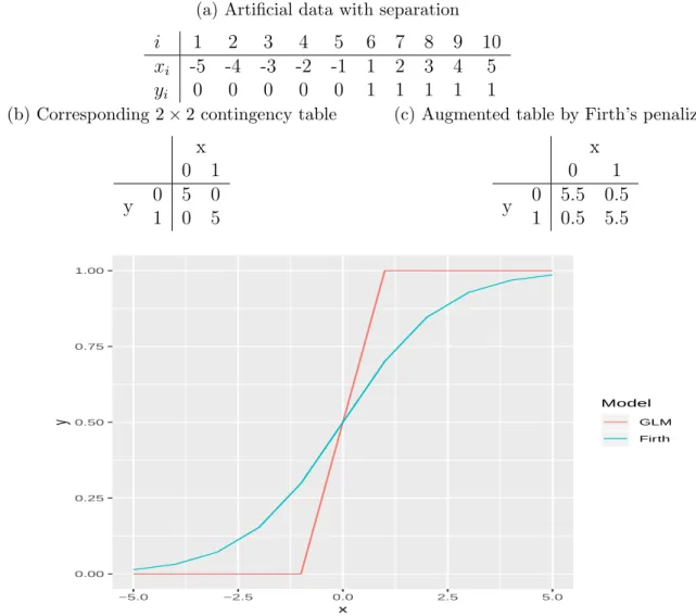
Recent developments in the statistical literature have seen the emergence of newer methods for circumventing the estimation challenges posed by rare events when using logistic regression in the frequentist framework (Mansournia et al. (2018)). A method based on the penalization of likelihood function using the information matrix was proposed by Firth (1993). The original motivation for the method is the reduction of bias and mean square-error relative to the MLE. It has been adapted to mitigate the effect of separation and monotone likelihood in binary and survival models respectively (Heinze & Schemper 2002, Heinze & Schempe 2001). An intuitive explanation of complete separation and application of the Firth method is as follows. Consider the case of 10 observations with a single predictorX (positive values denoted as 1 and negative values denoted as 0) and a binary response Y, where yi = 0 whenever xi is negative and 1
otherwise,i= 1, . . . ,10 (see Table 1a). The implied two way table is given in Table 1b. Clearly, the odds ratio is infinite using maximum likelihood (ML) on this data. Firth’s penalization however, is equivalent to ML estimation after augmentation of the cell counts by 0.5 (see Table 1c). This amended estimator has been described elsewhere (see (Agresti 2002, p. 70-71)). In this case, the odds ratio is finite and thus have merits in modelling PD where probability of separation is high. Figure 1 shows the plots of the fitted probabilities from standard and Firth logistic regression models using the data. The Firth method showed better predictions than the unrealistic heaviside function produced by the logistic regression model.
The concept and importance of events per variable (EPV) requirements for developing accurate prediction model has been underemphasized in the literature on credit scoring. EPV is the simple ratio of the number of the less frequent outcome and the number of estimated regression coefficients, and thus useful for quantifying the amount of information in the data relative to model complexity. The aim of this paper is therefore to evaluate the performance of statistical approaches for rare events and EPV requirements for accurate predictions in credit scoring. Since statistical models for rare events are rarely used in this framework, we compared Firth (1993) method (Firth), modification of Firth logistic regression called Firth’s logistic regression with added covariate (FLAC- proposed by Puhr et al. (2017)) and logistic regression penalized by log-F prior (LF22- by Greenland & Mansournia (2015)) with methods such as linear discriminant analysis (LDA), Ridge regression (Ridge), GEV model and logistic regression (logit). In particular, we “balanced” the data using ROSE (Random Over-Sampling Examples, by Menardi & Torelli (2014) and Lunardon et al. (2014)) and SMOTE (Synthetic Minority Over-Sampling Technique, by Chawla et al. (2002)) methods for various EPV values and develop prediction models using logistic regression. Since the main reason for modellingPD is to predict loan applicants who have the tendency to default, we focus on model evaluation criteria for predictions in the context of regression analysis rather than classification. This is to ensure that the predictive performance measures are not threshold dependent. We also corrected the performance measures for overfitting both in the simulation study and data analysis. The approach we adopted for model validation is based on the bootstrap internal validation method which has been recommended for the validation of prediction models in small sample (Smith et al. (2014)).
The rest of the paper is organized as follows. In Section 2, we describe the data used in the study. The models and methods are reviewed in Section 3. We also provided brief explanations of the model evaluation criteria. In Section 4, we described the simulation study and the two methods of data balancing considered in the article. The results from the simulation study are also analysed. Results from the real data example is presented in Section 5 and conclusions are given in Section 6. We present results of apparent performance of the models and sample codes in the Appendix.
2
Data set
We used the Taiwan credit card data set (Yeh & Lien (2009)) in this study. The data is used in the simulation study to evaluate sample size requirements for adequate predictions when the number of variables and prevalence (event rate) are taken into account.
Table 1: Example of complete separation and Firth correction in a 2×2 contingency table
(a) Artificial data with separation i 1 2 3 4 5 6 7 8 9 10
xi -5 -4 -3 -2 -1 1 2 3 4 5
yi 0 0 0 0 0 1 1 1 1 1
(b) Corresponding 2×2 contingency table
x 0 1 y 0 5 0 1 0 5
(c) Augmented table by Firth’s penalization
x 0 1 y 0 5.5 0.5 1 0.5 5.5 0.00 0.25 0.50 0.75 1.00 −5.0 −2.5 0.0 2.5 5.0 x y Model GLM Firth
Figure 1: Predicted probabilities from classical logistic regression and logistic model using Firth method
2.1
Taiwan Credit Card data
The data set is from credit card clients from a bank in Taiwan, who is a cash and credit card issuer. The data is available within the University of California Irvine (UCI) machine learning repository. There are 30,000 observations in the data with 6636 (22.12%) defaulters. The outcome of interest is default payment (Yes = 1, No = 0). In the same vein as Yeh & Lien (2009), we used the following 23 variables in the models.
(a) Limit bal: Given credit amount (NT dollar). This include both the individual applicant credit and his/her family (supplementary) credit
(c) Education: 1 = graduate school; 2 = undergraduate; 3 = high school; 4 = others. We combined both groups 3 and 4 for this study
(d) Marital Status: 1 = married; 2 = single; 3 = others. The “others” category is small so, we combined groups 2 and 3
(e) Age(year)
(f) Pay 0 - Pay 6: History of past payment. Past monthly payment records tracked from April to September 2005 as follows: Pay 0= repayment status in September, 2005; Pay 2
= repayment status in August, 2005; . . . ; Pay 6 = repayment status in April, 2005. The measurement scale for the repayment status is -1 = pay duly; 1 = payment delay for one month; 2 = payment delay for two months; . . . ; 8 = payment delay for eight months; 9 = payment delay for nine months and above. We take this as ordinal variable.
(g) Bill Amt1 - Bill Amt6: Amount of bill statement (NT dollar). Bill Amt1 = amount of bill statement in September, 2005;Bill Amt2= amount of bill statement in August, 2005; . . . ; Bill Amt6 = amount of bill statement in April, 2005
(h) Pay Amt1-Pay Amt6: Amount of previous payment (NT dollar). Pay Amt1= amount paid in September, 2005; Pay Amt2 = amount paid in August, 2005; . . . ; Pay Amt6 = amount paid in April, 2005.
The continuous variables in the data are log-transformed to cushion the effect of skewness.
3
Models and Predictive accuracy measures
3.1
Models
The main criteria for the choice of models considered in this section is to assess the performance of newer statistical methods for rare events in the framework of modelling PD. The newer methods evaluated are Firth, FLAC and LF22 models, and are evaluated alongside LDA, GEV model and Ridge regression.
We assume there are n loan applicants with two possible events- default or non-default which is governed by a Bernoulli random variable Yi ∈ {0,1}, i = 1, . . . , n. The event of
interest is Y = 1, the positive event of defaults, with associated PD, π = P(Y = 1|X = x). The p-dimensional applicants attributes, X (covariates) include personal details, past credit history and behavioral data. The statistical problem is to estimate π =P(Y = 1|X =x) and a commonly used method is the logistic regression.
3.1.1 Logistic Regression
Logistic regression assumes that the probability of default,πis a linear function of the observed covariates. That is,
π =P(Y = 1|X=x) = exp(β0x).1 + exp(β0x),
wherex= (1, x1, . . . , xp) is the design matrix andβ = (β0, β1, . . . , βp) is the (p+1) dimensional
vector of regression parameters. The decision boundary is linear via the linear predictor,
lp = β0x. Thus, lp > 0 (equivalently {x : ˆπ > 0.5}, where ˆπ is the fitted probability) is classified as 1 and zero otherwise. In addition to its instability in modelling rare event data and well separated classes, it does not work well with non-linear effects of the covariates. The log-likelihood function for n subjects, which is not optimized for predictions, is given by
l(β) = n X i=i h yi β0xi −log 1 + exp(β0xi) i . (1)
We evaluated the performance of logistic regression on the probability scale as a model for PD rather than as a classifier.
3.1.2 Firth (1993) Method
Firth’s penalized log-likelihood function for logistic regression can be written as
l(βF irth) =l(β) + 1/2 log|I(β)|,
where l(β) is the log-likelihood function in equation (1) and |I(β)| is the determinant of the Fisher information matrix. Alternatively, parameter estimates can be obtained by solving the modified score equation:
n X i=1 n yi−πi+hi( 1 2 −πi) o xir = 0; r= 0, . . . , p, (2)
where hi is thei-th diagonal elements of the hat matrix H =W1/2X(X0WX)−1XW1/2,W is
the diagonal matrix diag{πi(1−πi)} and p is the dimension of the covariates. Consequently,
the Fisher information matrix, I(β) =X0WX. The estimator prevents bias in the MLEs and produce useful standard errors. This is because the penalizing factor contains information on
the curvature of the likelihood function and thus contains information on the variation of the coefficient estimates. The penalty term is asymptotically negligible in large data sets, and thus coefficient estimates from the Firth estimator coincides with the ML. A major disadvantage of using Firth estimator for prediction in rare events setting is that it introduces bias in predicted probabilities towards π = 0.5 (Puhr et al. (2017)). This is because the determinant of the Fisher information matrix is maximized for π = 0.5 and thus push the predicted probabilities towards 0.5 compared with the MLE.
3.1.3 Firth’s Logistic regression with Added Covariate (FLAC)
Puhr et al. (2017) proposed the FLAC approach to overcome the bias problem in average predicted probabilities of the Firth estimator. The method involves the following steps:
1. Apply Firth’s logistic regression and calculate the diagonal elementshi of the hat matrix.
2. Construct an augmented data set by stacking: (i) the original observations weighted by 1,
(ii) the original observations weighted by hi/2 and
(iii) the original observations weighted by hi/2 but with reversed values of the binary
outcome variable (yi replaced by 1−yi).
3. Define an indicator variable g on this augmented data set, where for (i) g = 0 and for (ii) and (iii) g = 1.
4. The FLAC estimates are then obtained by ML estimation on the augmented data set adding g as covariate.
Following from equation (2), the FLAC method has a modified score equation given as
n X i=1 (yi−πi)xir | {z } Original data + n X i=1 hi 2(yi−πi)xir | {z }
Original data, weighted byhi/2
+ n X i=1 hi 2(1−yi −πi)xir | {z }
Data with reversed outcome
| {z }
Pseudo data
= 0.
g = 0 g = 1 (indicator variable)
The FLAC method, like the Firth method, circumvents the problem of separation in low EPV settings.
3.1.4 log-F Prior Penalty
The Firth penalty is data dependent since it is proportional to exp(1/2 ln|I(β|)) and I(β) is composed of the design matrix of the observed covariates. Consequently, the covariates can induce correlations in the penalty term as well as in the coefficient estimates. These artifactual prior correlations lead to a serious practical defect of the Firth penalty. In order to circumvent this problem, Greenland & Mansournia (2015) proposed a class of penalty functions which is not data dependent. The method is developed in the Bayesian framework but can be easily implemented in any logistic regression package by translating each desired coefficient penalty into a pseudo record data. For example, letβ1 be an element ofβ, withx1 as the corresponding
element ofx. Because a log-F(m, m) density is proportional toemβ1/2/(1 +eβ1)m, penalization
of β by a log-F(m, m) prior can be performed by adding a data record with m/2 successes on
m trials. In general, the prior degrees of freedom m in a log-F prior is exactly the number of observations added by the prior. Penalization by log-F(m, m) priors is in general equivalent to multiplying the likelihood function corresponding to equation (1) by emβ/2/(1 +eβ)m. The
log-likelihood function is therefore
l(βLF22) =l(β) +mβ/2−mlog(1 +eβ).
When m = 0, the function reduces to the log-likelihood function in equation (1). Greenland et al. (2016) suggested the use of log-F prior as a default prior for the general sparse-data settings. We consider m = 2 (denoted as LF22 method) for this study.
3.1.5 Ridge Regression
The ridge method minimizes the mean squared error of predictions by introducing some bias to the estimates of the regression coefficients. The log-likelihood function in equation (1) can be reconstructed as a constrained likelihood problem, where l(β) is maximized subject to
Pp
j=1β 2
j ≤ t; t ≥ 0, where t is a scalar chosen by the investigator. Equivalently, the ridge
penalized likelihood function can be written as
l(βRidge) = l(β)−λ
p
X
j=1
βj2, (3)
where λ≥0 has a one-to-one correspondence with t, and it is referred to as the regularization parameter, βRidge are the parameter estimates from the ridge regression. The larger the value
of λ, the further the parameter estimates are shrunk towards zero. In particular, the standard logistic regression is recovered when λ= 0 in (3). The ridge estimator is a convex optimization
problem and it is sometimes referred to as an L2-type regularization procedure (Verweij &
Van Houwelingen (1994)). Except for cases of complete separation, the ridge estimator will converge.
3.1.6 Linear Discriminant Analysis (LDA)
LDA, also known as Fisher’s LDA (Fisher (1936)), is a widely used method aimed at finding linear combinations of observed attributes,Xwhich best separate two or more classes of events. For credit scoring, LDA assumes that there is a prior probability, P(Y = 1) = π?, of default and that the conditional distribution ofP(X =x|Y =j)∼N(µj,Σ),j ={0,1}, a multivariate
normal with µj and covariance matrix Σ. Using Baye’s theorem,
P(Y = 1|X =x) = π ?exp(−1 2d1(x)) π?exp(−1 2d1(x)) + (1−π?) exp(− 1 2d0(x)) ,
where dj = (x−µj)0Σ−1(x−µj) is the Mahalanobis distance from x to µj. Since the decision
boundary is linear, the log-odds can be computed as
log P(Y = 1|X =x) P(Y = 0|X =x) = log π? 1−π? − 1 2(µ1+µ0) 0 Σ−1(µ1−µ0) +x0Σ−1(µ1−µ0) =β0x.
The predicted probabilities using the linear predictor are available in all major statistical software.
3.1.7 Generalized Extreme Value (GEV) regression model
The GEV model has been used to estimate and predict extreme events in many applications such as environment, engineering, economics and finance. Calabrese & Osmetti (2013) pro-posed its use for modelling PD. The cumulative distribution function is given by
F(x) = expn−h1 +ξx−µ σ
i−1/ξo
− ∞< ξ <∞, −∞< µ <∞, σ > 0,
defined on the support S = {x : 1 + ξ((x −µ)/σ) > 0}. The parameter ξ is the shape parameter, µ and σ are the location and scale parameters respectively. The probability of default is π(xi) = exp{−[1 +ξ(β0xi)]−1/ξ}. The corresponding linear predictor can be derived
{−ln[π(xi)]}−ξ−1
ξ =β
0x
i.
We fitted this model using the GJRM (Generalised Joint Regression Modelling) package in R statistical software (Marra & Radice (2017)).
3.2
Criteria for predictive performance
Brier score (BS): It is a measure of agreement between the observed binary outcome (i.e., default vs. non-default) and the predicted PD (Brier (1950)). We used brier score plus (BS+
- brier score computed for only the positive outcome).
Area under the receiver operating curve (AUROC): The generalization of the AUROC
is the c-index (Harrell et al. (1982)). It is a measure of model performance that separates sub-jects with the event of interest from subsub-jects without the event (discrimination). It calculates the proportion of pairs in which the predicted event probability is higher for the subject with the event of interest than that of the subject without the event. A model with no discriminatory ability has value around 0.5 whereas a value close to 1 suggests excellent discrimination.
Area under the Precision-Recall curve (AUPRC):The Precision-Recall curve shows the relationship between precision (P(Y = 1|Yˆ = 1)), where ˆYi are fitted values, and recall (P( ˆY =
1|Y = 1)) for every possible threshold values. It takes into account the prior probability of the outcome of interest. The AUPRC is therefore a summary statistic that reflects the ability of a classifier to identify the minority group. Unlike the AUROC, it values ranges from 0 to 1. Its value approaches zero as the prior probability of the outcome decreases. Davis & Goadrich (2006) recommended its use over AUROC in rare event and class imbalance data settings.
Calibration slope (CS):The slope is used to check the agreements between the observed and predicted probabilities. We regressed the binary outcome on the linear predictors obtained from the models using logistic regression (except for the GEV regression model where the regression was done using the GEV model). The resulting slope in this regression is the calibration slope. A slope of one suggests perfect calibration (Cox (1958)).
4
Simulation based on the Taiwan credit card data set
4.1
Simulation settings
We used the Taiwan credit card data as the basis for the simulation and varied the prevalence and EPV. Let Yi (outcome) and xi (covariates) be defined as in Section 3.1. The assumed
regression model for the data (suppressing index, i) is of the form logit(E(Y)) = β0x. We simulated the training data sets using the steps in Pavlou et al. (2016) as follows.
1. Fit a logistic regression model to the original data set to obtainβˆ0 = ( ˆβ
0,βˆ1) where ˆβ0
is the estimate of the intercept term and βˆ1 is the estimate of the vector of regression
coefficients for the covariates.
2. Choose the required prevalence (prev) and replace ˆβ0 by the value ˆβ0∗ that makes the
average fitted probability equal to prev. Define β∗0= ( ˆβ0∗,βˆ1).
3. To create the data, choose the EPV and prev, and calculate sample size for each EPV given the number of covariates p. The sample size is given by n = EPV×p
prev . Sample
with replacementn values of the covariates in the true model from the original data and generate a new outcome Ysim ∼ Bernoulli(logit−1(β∗0x)). The resulting data set of size
n is (Ysim, x) and the process is repeated to produce 500 training data sets (number of
replication).
We considered prevalence of 5%, 10% and 20% (22.12% is the prevalence of the entire data set). The models are evaluated on EPV= {2, 3, 5, 7, 10}, with EPV of 10 recommended for model accuracy (Peduzzi et al. (1996)). Each of the models developed in the training samples are validated using the bootstrap validation method (Harrell et al. (1996)). The steps for the model validation are as follows.
(a) Simulate the data set based on the required EPV. Fit the models using the methods in section 3.1 and compute Apparent predictive performance based on the performance measure of interest, sayAU ROCapp.
(b) Take B bootstrap samples from the simulated data set, whereb = 1. . . B. Fit the models and compute AU ROCboot(b) . This is the bootstrap performance.
(c) Test the performance of each of theB models on the original simulated data by computing
(d) Optimism in model fit for each of the bootstrap sample isOpt(b)=AU ROC(b)
boot−AU ROC (b) orig.
The average optimism is
Opt=
PB
b=1Opt(b)
B .
(e) Optimism corrected measures for the original model isAU ROCcorrect =AU ROCapp−Opt.
We take B = 150 for this study.
4.2
SMOTE and ROSE techniques for data balancing
In addition to the models examined in Section 3.1, we evaluated the use of SMOTE and ROSE methods for data balancing.
SMOTE: The technique generates randomly new examples or instances of the minority class from the nearest neighbours of line joining the minority class sample to increase the number of instances. These instances are created based on the features of the original data set so that they are similar to the original instances of the minority class (Chawla (2005)).
The SMOTE algorithm can be constructed as follows. For each minority class instancex:
1. Compute its nearest neighbours, sayk = 5 neighbours. 2. Randomly choose one of the neighbours, say x∗.
3. Create a synthetic new minority sample, xnew using x0s feature vector and the feature
vector’s difference of x∗ and x multiplied by a random number from the uniform distri-bution.
That is,
xnew =x+u.(x∗−x),
where u ∼ U(0,1). We kept the proportion r = |m|/|M| to 0.75, where r is the ratio of the number of examples in the minority class (m) to the number in the majority class (M).
ROSE: The method is based on the generation of new artificial data according to a smoothed bootstrap approach. The method is as follows.
Let P(x) = f(x) be the probability density function on X. Let nj < n be the size of
1. select y=Yj, j ∈ {0,1}, with probability 1/2.
2. select (xi, yi) in the sample such that yi =y with probability pi = 1/nj.
3. sample the vector of covariates x from the kernel probability distribution KHj(·,xi)
centered on xi and depending on the matrix of smoothing parametersHj.
That is, an observation belonging to one of the two classes is drawn from the training set with the same probability. A new sample is then generated in its neighborhood of width governed by Hj. Further details on how to select the smoothing matrix Hj can be found in
Menardi & Torelli (2014) and Lunardon et al. (2014).
We used similar bootstrap steps in section 4.1 to correct for overfitting in the models. Here, the training data sets are first “balanced” using either SMOTE or ROSE techniques. The balanced data is then used in the bootstrap steps to develop models for PD using logistic regression. The original imbalanced data (test data) is used to test predictive accuracy of the developed models in the bootstrap samples.
Simulation results
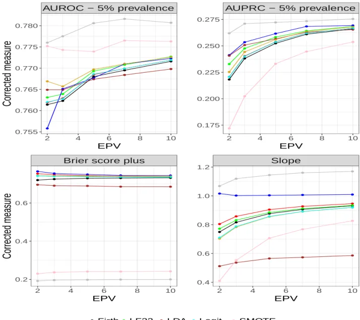
Figures 2-4 shows the predictive performance of the methods for different values or prevalence. When the prevalence is 5% (Figure 2), ROSE data balancing method outperforms the other methods on discrimination as shown by AUROC and AUPRC. The SMOTE method, another data balancing technique, shows the second best discriminatory ability on AUROC but pre-forms poorly on AUPRC. Of the three Firth-type penalization methods, the LF22 is superior to Firth and FLAC methods on AUROC. Although GEV model performs well on AUROC, its estimates are not generally stable at EPV=2, resulting in AUROC estimates for EPV=2 being greater than EPV = 3. The FLAC method is practically indistinguishable from the logit. However, both methods show better discrimination than the Firth method at EPV≤5. This is in line with the submission in Puhr et al. (2017), where the authors opined that Firth method introduces bias in predicted probabilities. Ridge on the other hand does not perform well at EPV=2 when AUROC is used to evaluate discrimination. However, it exhibits gradual improvement until it surpasses the other methods (except ROSE and SMOTE) at EPV ≥ 7. Again, Ridge performs well on AUPRC, where it is outperformed only by ROSE.
In terms of calibration, the Ridge is the best performing method as shown by the calibration slope (value of 1 indicates perfect calibration). The slope is better calibrated for FLAC than Firth and LF22 models. The GEV model and logit are indistinguishable on this performance measure. However, LDA is poorly calibrated. This may be due, in part, to the use of logistic model for the computation of the calibration slope as described in Section 3.2. Figure 2 (bottom
left) shows the BS+ computed on the defaulters. Overall, ROSE has the least error followed
by SMOTE. Among the Firth-type method, Firth method is the best. This is not surprising as the method is generally known to have low mean square error. Although Ridge outperforms Firth when the standard Brier score is used (result not shown), its performance is the worst on BS+. AUROC − 5% prevalence 2 4 6 8 10 0.755 0.760 0.765 0.770 0.775 0.780 EPV
Corrected measure
AUPRC − 5% prevalence 2 4 6 8 10 0.175 0.200 0.225 0.250 0.275 EPVBrier score plus
2 4 6 8 10 0.2 0.4 0.6 EPV
Corrected measure
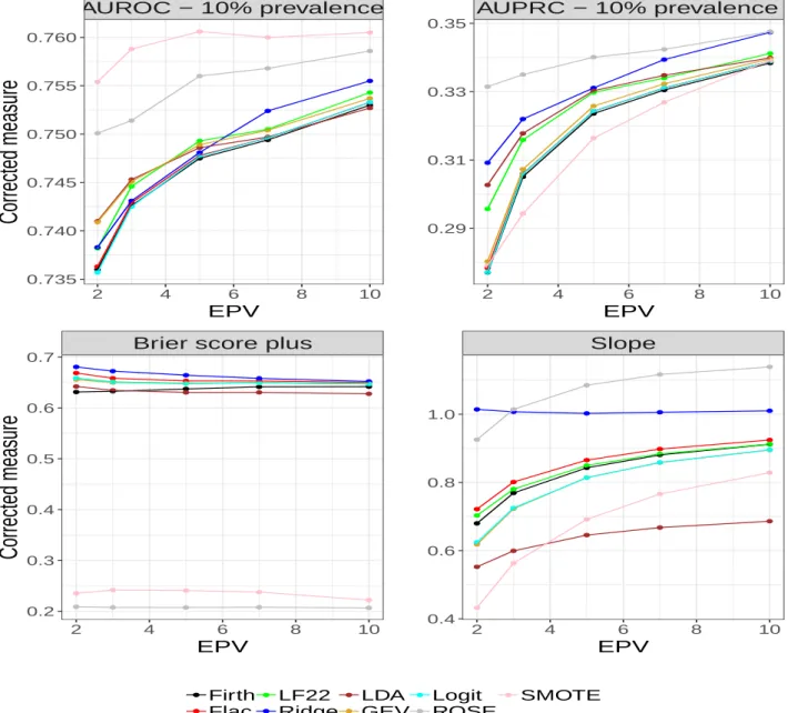
Slope 2 4 6 8 10 0.4 0.6 0.8 1.0 1.2 EPV Firth Flac LF22 Ridge LDA GEV Logit ROSE SMOTEFigure 2: Optimism corrected predictive accuracy measures for prevalence of 5% Some of the methods compared improved as prevalence of the outcome variable increases. from 5% to 10% (see Figure 3). Again, both ROSE and SMOTE perform well on AUROC, but the SMOTE technique is superior. Similar to the results in Figure 2, Ridge becomes in-creasingly better from EPV = 2 and outperforms other methods (except ROSE and SMOTE) at EPV > 5 when AUROC is the performance measure of interest. The more stable AUPRC
ranked ROSE and Ridge as the best among the methods. The performance of SMOTE im-proved from prevalence of 5% to 10%. The performance of the methods on calibration slope and BS+ follow the same pattern as shown in Figure 2 for the prevalence of 5%.
AUROC − 10% prevalence 2 4 6 8 10 0.735 0.740 0.745 0.750 0.755 0.760 EPV
Corrected measure
AUPRC − 10% prevalence 2 4 6 8 10 0.29 0.31 0.33 0.35 EPVBrier score plus
2 4 6 8 10 0.2 0.3 0.4 0.5 0.6 0.7 EPV
Corrected measure
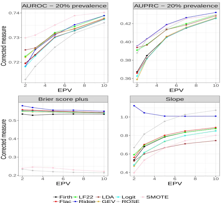
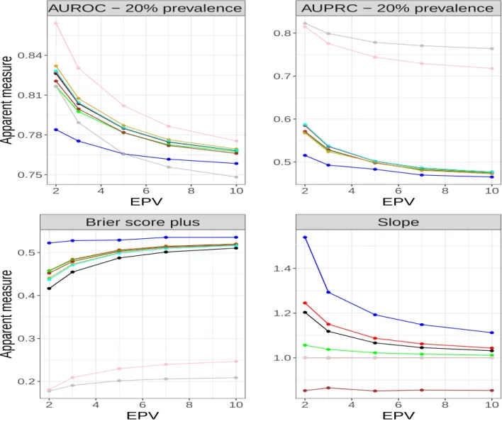
Slope 2 4 6 8 10 0.4 0.6 0.8 1.0 EPV Firth Flac LF22 Ridge LDA GEV Logit ROSE SMOTEFigure 3: Optimism corrected predictive accuracy measures for prevalence of 10% The results of model performance at prevalence of 20% are shown in Figure 4. SMOTE maintained a strong discriminatory ability on AUROC but ROSE deteriorated. Its performance on AUROC is consistent across the three event rates. On the other hand, ROSE and Ridge perform consistently well across the three levels of prevalence and EPV values considered for AUPRC (Figure 5). The LF22 model performs consistently better than the Firth, FLAC, GEV model and logit on AUROC and AUPRC. Again, the performance of the methods on calibration slope and BS+ follow the same pattern as seen in Figures 2 and 3. While the slope
for Ridge get closer to 1 as EPV approaches 6, it approaches 1 as EPV increases for SMOTE. AUROC − 20% prevalence 2 4 6 8 10 0.72 0.73 0.74 EPV
Corrected measure
AUPRC − 20% prevalence 2 4 6 8 10 0.36 0.38 0.40 0.42 EPVBrier score plus
2 4 6 8 10 0.2 0.3 0.4 0.5 EPV
Corrected measure
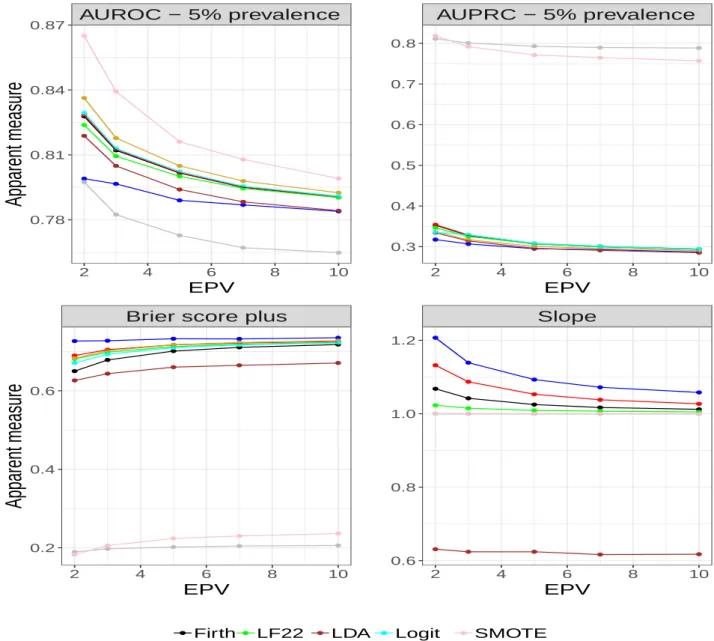
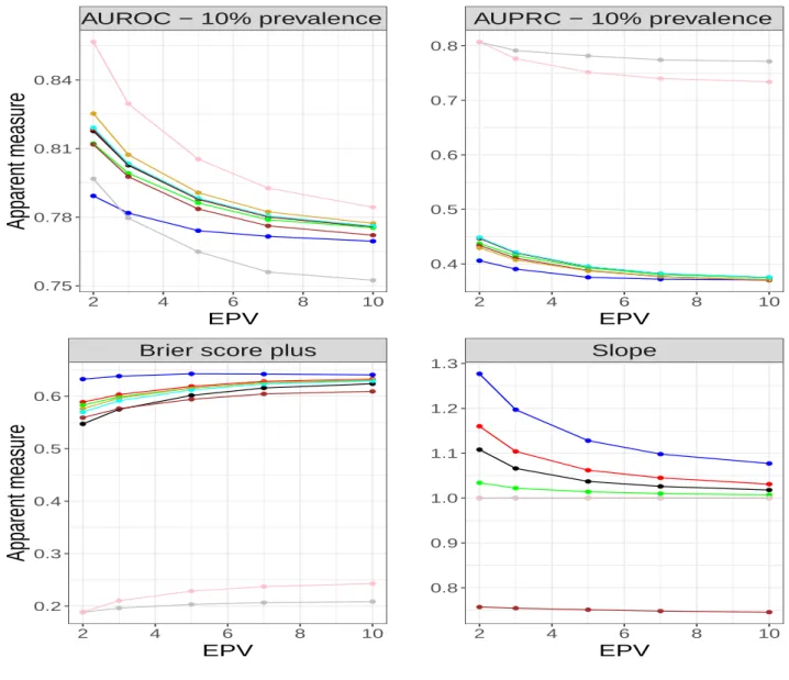
Slope 2 4 6 8 10 0.4 0.6 0.8 1.0 EPV Firth Flac LF22 Ridge LDA GEV Logit ROSE SMOTEFigure 4: Optimism corrected predictive accuracy measures for prevalence of 20% Figures 6- 8 (Appendix A) shows the results of apparent performance measures from the simulation study. All the Figures show high degree of overfitting especially at low EPV. In particular, Figures 6- 8 (top, left) shows that Ridge does not perform well when the model is not adjusted for optimism. In principle, this model is the least susceptible to overfitting. Also, there is severe overfitting in models developed with ROSE and SMOTE on AUPRC across the event rates. This corroborates the importance of internal validation of predictive models.
EPV2 − AUPRC 5 10 15 20 0.20 0.25 0.30 0.35 0.40 Prevalence (Percentage)
Corrected measure
EPV5 − AUPRC 5 10 15 20 0.25 0.30 0.35 0.40 Prevalence (Percentage) EPV7 − AUPRC 5 10 15 20 0.25 0.30 0.35 0.40 Prevalence (Percentage)Corrected measure
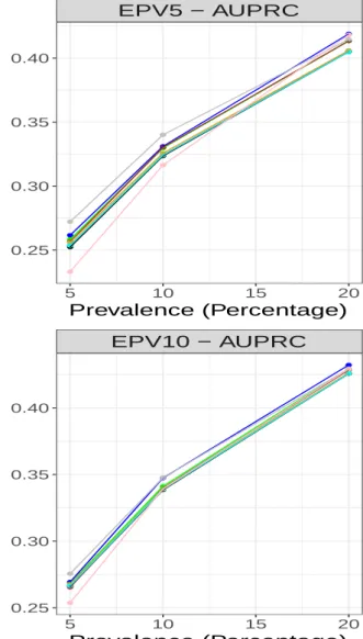
EPV10 − AUPRC 5 10 15 20 0.25 0.30 0.35 0.40 Prevalence (Percentage) Firth Flac LF22 Ridge LDA GEV Logit ROSE SMOTEFigure 5: Comparison of predictive performance on AUPRC across prevalence
5
Data Analysis
We used the Taiwan credit card data described in section 2 to evaluate the performance of our models. In the data, the higher the amount of credit given, the higher the probability of default. In particular, all applicants older than 50 years of age borrowed 620,000 Taiwanese dollars or more, and they are defaulters. Age does not affect the chance of paying back amount borrowed that is less than 500,000 dollars.
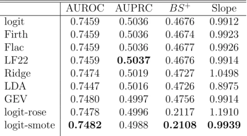
The results from fitting the models are summarized in Table 2. Logistic regression with data balancing technique using SMOTE slightly outperforms the other methods on three out of the
four measures of predictive accuracy (AUROC, BS+ and Calibration slope). The performance
of Firth, FLAC and the LF22 methods (Firth-type penalization) are essentially the same. This is expected since the sample size is now large (EPV = 289). The GEV model outperforms the logit on AUROC and BS+, which is in line with previous observation (Calabrese & Osmetti (2013)). It should be noted that the performance of SMOTE using AUROC is in concord with our observation from the simulation study. That is, the method is very good when AUROC is used for discrimination regardless of prevalence and corresponding EPV values. One noticeable result is the performance of SMOTE on calibration slope. Again, this follows from the simulation study, whereby AUROC value approaches 1 as EPV increases.
Table 2: Model performance in predicting default probability in Taiwan credit card data AUROC AUPRC BS+ Slope
logit 0.7459 0.5036 0.4676 0.9912 Firth 0.7459 0.5036 0.4674 0.9923 Flac 0.7459 0.5036 0.4677 0.9926 LF22 0.7459 0.5037 0.4676 0.9914 Ridge 0.7474 0.5019 0.4727 1.0498 LDA 0.7447 0.5016 0.4726 0.8975 GEV 0.7480 0.4997 0.4756 0.9914 logit-rose 0.7478 0.4996 0.2117 1.1910 logit-smote 0.7482 0.4988 0.2108 0.9939
6
Concluding remarks
This paper examined six modifications of the logistic regression (Firth, FLAC, LF22, Ridge, ROSE and SMOTE), linear discriminant analysis (LDA) and binary regression model using generalized extreme value distribution (GEV) in the estimation of probability of default (PD). The simulation study is based on the modification of event rate in the Taiwan credit card data. We evaluated measures of model performance identified in the literature for the evaluation of predictive accuracy in class imbalanced data settings. Sample size was taken into account in the evaluation of the methods using events per variable (EPV). Since the design factors (number of predictors and event rate) are kept constant, both EPV and sample size have one-to-one correspondence and the same conclusion is expected.
The key result showed that SMOTE should be preferred when the aim is to obtain op-timal discrimination using AUROC in small and large samples. SMOTE exhibited patterns of improved predictive accuracy as EPV increases on three of the measures of performance (AUROC, BS+ and Slope). In particular, the slope approaches 1 as EPV becomes large. This
is further corroborated in the data analysis where EPV equals 289. For optimal performance on AUPRC, we recommend the use of ROSE and ridge regression. Of the statistical methods analyzed, the LF22 and FLAC methods are generally superior to Firth, logit and GEV models. In addition, the two models converge and will generally produce accurate predictions in the presence of sparse data structure (e.g. binary predictors with low prevalence), whereas models such as GEV and logistic regression are likely to fail in such setting. Although the computa-tional time is higher for FLAC and LF22 models than the logit model, improved predictive accuracy in small sample cannot be traded for computational complexity.
The measure of predictive accuracy based on AUPRC appears to be a more realistic measure of discrimination than AUROC in rare event settings. As can be seen from Figure 5, the performance of all the methods increases on this measure from 5% prevalence to 20% as expected. Consider the ridge regression for example, the corrected AUPRC at EPV = 2 for 5% prevalence is 0.2412. This value increases to 0.3092 for 10% prevalence and 0.3954 for 20% prevalence. On the other hand, and at EPV = 2 the AUROC values are 0.7558, 0.7383 and 0.7183 for 5%, 10% and 20% prevalence respectively, indicating consistent decline across prevalence.
A possible criticism of the bootstrap method used for internal validation is the possibilities of model non-convergence within the bootstrap samples for models such as logistic regression and GEV models. As noted by Loughin (1998), separation has significant probability of occurring in resamples when the event of interest is rare. Whilst this argument may be valid in certain cases, the chance of not selecting any member of the minority group is just approximately
1/3. We accommodated the possibility of such divergence/singularity in the resample. We also emphasized the merits of model evaluation in simulation studies using optimism corrected measures (Ogundimu & Collins (2018)).
Although we showed the conditions for preference of SMOTE and LF22 methods on the data, the latter can be improved to cater for various modelling challenges that are often encountered while modelling PD. For example, the method can be combined with the ridge method (in a similar way as Shen & Gao (2008) combined Firth and Ridge methods) to optimize predictive accuracy of PD. In addition to optimized predictive accuracy, this method will alleviate the effect of multicollinearity- a common problem in credit scoring. We have combined both undersampling of the majority class and oversampling of the minority class to achieve a ratio of 0.75 for data balancing using SMOTE. This is not necessarily optimal as SMOTE can be used without undersampling. The performance of SMOTE can also be improved by developing sampling strategy such that the amount of oversampling and the nearest neighbours used for a particular data is selected in some optimal way. There are still open questions on variable selection and methods for dealing with incomplete data in credit scoring. SMOTE (and its variants) and LF22 methods have enormous potential in these settings.
References
Agresti, A. (2002), Categorical data analysis, second edn, John Wiley & Sons Ltd, New York. Altman, E. (1968), ‘Financial ratios, discriminant analysis and the prediction of corporate
bankruptcy’,J. Finance. 23(4), 589–609.
Basel Committee on Banking Supervision (June, 2004), International convergence of Capital
Measurement and Capital Standards: A Revised Framework.
Berk, R. A. & Bleich, J. (2013), ‘Statistical procedures for forecasting criminal behavior: A comparative assessment’, Criminol. Public Policy. 12(3), 513–544.
Brier, G. W. (1950), ‘Verification of forecasts expressed in terms of probability’, Mon. Weather Rev. 78, 1–3.
Calabrese, R. & Osmetti, S. A. (2011), ‘Generalized extreme value regression for binary rare events data: an application to credit defaults’, Discussion Paper.
Calabrese, R. & Osmetti, S. A. (2013), ‘Modelling small and medium enterprise loan defaults as rare events: the generalized extreme value regression model’, J. Appl. Stat. 40(6), 1172– 1188.
Chawla, N. V. (2005), Data mining for imbalanced datasets: An overview, in O. Maimon & L. Rokach, eds, ‘Data mining and knowledge discovery handbook’, Springer, Boston, MA, pp. 853–867.
Chawla, N. V., Bowyer, K. W., Hall, L. O. & Kegelmeyer, W. P. (2002), ‘SMOTE: Synthetic Minority OverSampling Technique’, J. Artif. Intell. Res.16, 321–357.
Chen, M. (2004), Skewed link models for categorical response data,inM. G. Genton, ed., ‘Skew-Elliptical Distributions and Their Applications: A Journey Beyond Normality’, Chapman & Hall, CRC, Boca Raton, Florida, pp. 223–241.
Courvoisier, D. S., Combescure, C., Agoritsas, T., Gayet-Ageron, A. & Perneger, T. V. (2011), ‘Performance of logistic regression modeling: beyond the number of events per variable, the role of data structure’, J. Clin. Epidemiol 64, 993–1000.
Cox, D. R. (1958), ‘Two further applications of a model for binary regression’, Biometrika
45, 562–565.
Czado, C. & Santner, T. J. (1992), ‘The effect of link misspecification on binary regression inference’,J. Stat. Plan. Inference. 33(2), 213–231.
Davis, J. & Goadrich, M. (2006), The Relationship Between Precision-Recall and ROC Curves, in‘Proceedings of the 23rd International Conference on Machine Learning’, ICML ’06, ACM, New York, NY, USA, pp. 233–240.
Durand, D. (1941), ‘Risk elements in consumer installment financing’, New York: National
Bureau of Economic Research pp. 189–201.
Firth, D. (1993), ‘Bias reduction of maximum likelihood estimates’, Biometrika 80, 27–38. Fisher, R. (1936), ‘The use of multiple measurements in taxonomic problems’, Ann. Eugen.
7(2), 179–188.
Ghotra, B., McIntosh, S. & Hassan, A. E. (2015), ‘Revisiting the impact of classification techniques on the performance of defect prediction models’, In 37th ICSE-Volume 1. IEEE
Press pp. 789–800.
Greenland, S. & Mansournia, M. A. (2015), ‘Penalization, bias reduction, and default priors in logistic and related categorical and survival regressions’, Stat. Med. 34, 3133–3143. Greenland, S., Mansournia, M. A. & Altman, D. G. (2016), ‘Sparse data bias: a problem hiding
in plain sight’, BMJ.352, i1981.
Hand, D. J. & Henley, W. E. (1997), ‘Statistical classification methods in consumer credit scoring: A review’, J. R. Stat. Soc. Series A. 160(3), 523–541.
Harrell, F., Califf, R., Pryor, D., Lee, K. & Rosati, R. (1982), ‘Evaluating the yield of medical tests’, JAMA 247, 2543–2546.
Harrell, F. E., Lee, K. L. & Mark, D. B. (1996), ‘Tutorial in biostatistics, multivariable prog-nostic models: Issues in developing models, evaluating assumptions and adequacy, and mea-suring and reducing errors’, Stat. Med. 15, 361–387.
Heinze, G. & Schempe, M. (2001), ‘A solution to problem of monotone likelihood in Cox regression’, Biometrics 57, 114–119.
Heinze, G. & Schemper, M. (2002), ‘A solution to the problem of separation in logistic regres-sion’, Stat. Med. 21, 2409–2419.
King, G. & Zeng, L. (2001), ‘Logistic regression in rare events data’, Polit. Anal. 9, 137–163. Loughin, T. M. (1998), ‘On the bootstrap and monotone likelihood in the Cox proportional
hazards regression model’,Lifetime Data Anal. 4(4), 393–403.
Lunardon, N., Menardi, G. & Torelli, N. (2014), ‘ROSE: a package for Binary Imbalanced Learning’, R Journal 6(1), 79–89.
Mansournia, M. A., Geroldinger, A., Greenland, S. & Heinze, G. (2018), ‘Separation in logistic regression: causes, consequences, and control’,Am J Epidemiol. 187, 864–870.
Marra, G. & Radice, R. (2017), ‘A joint regression modeling framework for analyzing bivariate binary data in R’, Dependence Modeling 5(1), 268–294.
Menardi, G. & Torelli, N. (2014), ‘Training and assessing classification rules with imbalanced data’, Data Min. Knowl. Discov. 28(1), 92–122.
Ogundimu, E. O., Altman, D. G. & Collins, G. S. (2016), ‘Adequate sample size for developing prediction models is not simply related to events per variable’, J. Clin. Epidemiol.76, 175– 182.
Ogundimu, E. O. & Collins, G. S. (2018), ‘Predictive performance of penalized beta regression model for continuous bounded outcomes’,J. Appl. Stat. 45(6), 1030–1040.
Pavlou, M., Ambler, G., Seaman, S., De Iorio, M. & Omar, R. Z. (2016), ‘Review and evaluation of penalised regression methods for risk prediction in low-dimensional data with few events’,
Stat Med. 180(7), 1159–1177.
Peduzzi, P., Concato, J., Kemper, E., Holford, T. R. & Feinstein, A. (1996), ‘A simulation study on the number of events per variable in logistic regression analysis’,J. Clin. Epidemiol.
49, 1373–1379.
Puhr, R., Heinze, G., Nold, M., Lusa, L. & Geroldinger, A. (2017), ‘Firth’s logistic regression with rare events: accurate effect estimates and predictions?’,Stat. Med. 36(14), 2302–2317. Rainey, C. (2016), ‘Dealing with separation in logistic regression models’, Polit. Anal.
24(3), 339–355.
Shen, J. & Gao, S. (2008), ‘A solution to separation and multicollinearity in multiple logistic regression’, J. Data Sci.6(4), 515–531.
Smith, G. C., Seaman, S. R., Wood, A. M., Royston, P. & White, I. R. (2014), ‘Correcting for optimistic prediction in small data sets’,Am. J. Epidemiol. 180(3), 318–324.
Taylor, J. M. G., Siqueira, A. L. & Weiss, R. E. (1996), ‘The cost of adding parameters to a model’, J. R. Statist. Soc. B. 58(3), 593–607.
Thomas, L. C., Edelman, D. B. & Crook, J. N. (2002), Credit scoring and its applications, Society for Industrial and Applied Mathematics, Philadelphia.
Verweij, P. J. M. & Van Houwelingen, H. C. (1994), ‘Penalized likelihood in Cox regression’,
Weiss, G. M. (2004), ‘Mining with rarity: a unifying framework’, SIGKDD Explorations
Newsletter6(1), 7–19.
Yeh, I. & Lien, C. (2009), ‘The comparisons of data mining techniques for the predictive accuracy of probability of default of credit card clients’, Expert Syst Appl. 36, 2473–2480. Zorn, C. (2005), ‘A solution to separation in binary response models’, Polit. Anal.13(2), 157–
Appendix
A
Apparent Predictive Accuracy Measures
AUROC − 5% prevalence 2 4 6 8 10 0.78 0.81 0.84 0.87 EPV
Apparent measure
AUPRC − 5% prevalence 2 4 6 8 10 0.3 0.4 0.5 0.6 0.7 0.8 EPVBrier score plus
2 4 6 8 10 0.2 0.4 0.6 EPV
Apparent measure
Slope 2 4 6 8 10 0.6 0.8 1.0 1.2 EPV Firth Flac LF22 Ridge LDA GEV Logit ROSE SMOTEAUROC − 10% prevalence 2 4 6 8 10 0.75 0.78 0.81 0.84 EPV
Apparent measure
AUPRC − 10% prevalence 2 4 6 8 10 0.4 0.5 0.6 0.7 0.8 EPVBrier score plus
2 4 6 8 10 0.2 0.3 0.4 0.5 0.6 EPV
Apparent measure
Slope 2 4 6 8 10 0.8 0.9 1.0 1.1 1.2 1.3 EPV Firth Flac LF22 Ridge LDA GEV Logit ROSE SMOTEAUROC − 20% prevalence 2 4 6 8 10 0.75 0.78 0.81 0.84 EPV
Apparent measure
AUPRC − 20% prevalence 2 4 6 8 10 0.5 0.6 0.7 0.8 EPVBrier score plus
2 4 6 8 10 0.2 0.3 0.4 0.5 EPV
Apparent measure
Slope 2 4 6 8 10 1.0 1.2 1.4 EPV Firth Flac LF22 Ridge LDA GEV Logit ROSE SMOTEB
Sample R code for Internal validation
Bootstrap validation code for logistic regressionlogitboot <- function(formula, data, B, seed){ if (match("MASS",.packages(),0)==0) require(MASS) if (match("PRROC",.packages(),0)==0) require(PRROC) if (match("ROCR",.packages(),0)==0) require(ROCR) set.seed(seed) mf <- model.frame(formula, data) y <- model.response(mf, "numeric") X <- model.matrix(formula, data = data)
int <- slope <- auc <- pauc1 <- brier <- brierp <- cal <- c()
intest <- slopetest <- auctest <- pauctest1 <- briertest <- brierpt <- calt <- c()
# Looping to generate B bootstrap data bootdata <- mydat <- list()
for(i in 1:B){
iboot <- sample(1:nrow(data), replace=TRUE) bootdata[[i]] <- data[iboot,]
}
for(i in 1:B){ options(warn=2) dattest <- X
res <- try(glm(formula, data=bootdata[[i]], family=binomial(link = "logit"))) if (any(class(res)=="try-error")){
int[i] <- slope[i] <- auc[i] <- pauc1[i] <- brier[i] <- brierp[i] <- cal[i] <- NA intest[i] <- slopetest[i] <- auctest[i] <- pauctest1[i] <- briertest[i] <- NA brierpt[i] <- calt[i] <- NA
} else{
p <- res$fitted.values lp <- res$linear.predictors
mf2 <- model.frame(formula, bootdata[[i]]) yboot <- model.response(mf2, "numeric")
lptest <- dattest%*%coef(res) prtest <- plogis(lptest) fg <- p[yboot == 1] bg <- p[yboot == 0]
roc <- roc.curve(scores.class0 = fg, scores.class1 = bg) pr <- pr.curve(scores.class0 = fg, scores.class1 = bg)
ab <- glm(yboot~lp,family = binomial(logit))# usual calibration pred <- prediction(p, yboot)
int[i] <- ab$coef[1] slope[i] <- ab$coef[2] auc[i] <- roc$auc
pauc1[i] <- pr$auc.integral brier[i] <- mean((p-yboot)^2)
brierp[i] <- mean((p[yboot == 1]-yboot[yboot==1])^2)
cal[i] <- mean(unlist(performance(pred, "cal",window.size=100)@y.values))#sample size >100
# doing the test back in the original data fgt <- prtest[y == 1]
bgt <- prtest[y == 0]
roct <- roc.curve(scores.class0 = fgt, scores.class1 = bgt) prt <- pr.curve(scores.class0 = fgt, scores.class1 = bgt)
abt <- glm(y~lptest,family = binomial(logit)) predt <- prediction(prtest, y) intest[i] <- abt$coef[1] slopetest[i] <- abt$coef[2] auctest[i] <- roct$auc pauctest1[i] <- prt$auc.integral briertest[i] <- mean((prtest-y)^2)
brierpt[i] <- mean((prtest[y == 1]-y[y==1])^2)
calt[i] <- mean(unlist(performance(predt, "cal",window.size=100)@y.values)) }}
aaa <- auc
ck <- sum(is.na(aaa)) int <- mean(int, na.rm=T) slope <- mean(slope,na.rm=T) auc <- mean(auc,na.rm=T) pauc1 <- mean(pauc1,na.rm=T) brier <- mean(brier,na.rm=T)
brierp <- mean(brierp, na.rm=T) cal <- mean(cal, na.rm =T)
intt <- mean(intest, na.rm=T) slopet <- mean(slopetest, na.rm=T) auct <- mean(auctest,na.rm=T) pauct1 <- mean(pauctest1,na.rm=T) briert <- mean(briertest,na.rm=T) brierpt <- mean(brierpt, na.rm=T) calt <- mean(calt, na.rm =T)
# Index measures from the orginal data set options(warn=2)
orig <- try(glm(formula, data=data, family=binomial(link = "logit"))) if (any(class(orig)=="try-error")){
Oint <- Oslope <- Oauc <- Opauc1 <- Obrier <- Obrierp <- Ocal <-999 } else{
lporig <- orig$linear.predictors prorig <- orig$fitted.values fgo <- prorig[y == 1]
bgo <- prorig[y == 0]
oroc <- roc.curve(scores.class0 = fgo, scores.class1 = bgo) opr <- pr.curve(scores.class0 = fgo, scores.class1 = bgo)
oab <- glm(y~lporig,family = binomial(logit)) opred <- prediction(prorig, y) Oint <- oab$coef[1] Oslope <- oab$coef[2] Oauc <- oroc$auc Opauc1 <- opr$auc.integral Obrier <- mean((prorig-y)^2)
Obrierp <- mean((prorig[y == 1]-y[y==1])^2)
Ocal <- mean(unlist(performance(opred, "cal",window.size=100)@y.values)) }
index.orig <- c(Oint,Oslope,Oauc,Opauc1,Obrier,Obrierp,Ocal) training <- c(int,slope,auc,pauc1,brier, brierp,cal )
test <- c(intt,slopet,auct,pauct1,briert,brierpt,calt) data.a <- data.frame(index.orig,training,test)
data.a$optimism <- training-test
data.a$index.corrected <- index.orig-data.a$optimism data.a$n <- rep(B-ck, length(training))
data.a <- round(data.a,digits=4) xx <- c("int","slope","auc","pauc1","brier", "brierp","cal") rownames(data.a) <- xx outt <- list(nonconvergence=ck,resu=data.a) return(outt) }
This function can be easily extended to other model families as was done in this article. It can also be extended to include other desired measure of predictive accuracy. It gives exactly the same results as for the “validate.lrm” function in the rms package.
gendat <- function(n,seed){#data generation set.seed(seed)
beta = c(0.5, 0.5, 1,1,1,0) alpha<- -1.8
m <- length(beta)
X <- matrix(runif(n*m), nrow=n, ncol=m) Xb <- alpha + X%*%beta pr <- 1/(1+exp(-Xb)) y<- rbinom(n,1,pr) df <- data.frame(y,X) return(df) } dat <- gendat(1000,1) formula <- y~X1+X2+X3+X4+X5+X6 res <- logitboot(formula,data=dat,B=10,seed=1)
library(rms)# bootstrap validation in rms package
f <- lrm(y~X1+X2+X3+X4+X5+X6, x=TRUE, y=TRUE, data=dat) p <- predict(f,type="fitted",data =dat)
set.seed(1)
res
index.orig training test optimism index.corrected n int 0.0000 0.0000 0.0235 -0.0235 0.0235 10 slope 1.0000 1.0000 0.8715 0.1285 0.8715 10 auc 0.6467 0.6645 0.6433 0.0213 0.6254 10 pauc1 0.6493 0.6618 0.6455 0.0163 0.6330 10 brier 0.2327 0.2283 0.2345 -0.0062 0.2389 10 brierp 0.2287 0.2283 0.2361 -0.0078 0.2365 10 cal 0.0373 0.0491 0.0422 0.0069 0.0304 10 res.lrm
index.orig training test optimism index.corrected n Dxy 0.2933 0.3291 0.2865 0.0426 0.2507 10 R2 0.0924 0.1151 0.0876 0.0275 0.0649 10 Intercept 0.0000 0.0000 0.0235 -0.0235 0.0235 10 Slope 1.0000 1.0000 0.8715 0.1285 0.8715 10 Emax 0.0000 0.0000 0.0345 0.0345 0.0345 10 D 0.0708 0.0894 0.0670 0.0224 0.0484 10 U -0.0020 -0.0020 0.0019 -0.0039 0.0019 10 Q 0.0728 0.0914 0.0651 0.0263 0.0465 10 B 0.2327 0.2283 0.2345 -0.0062 0.2389 10 g 0.6392 0.7247 0.6203 0.1044 0.5347 10 gp 0.1506 0.1681 0.1467 0.0214 0.1292 10