Agricultural and Resource Economics Review 40/2 (August 2011) 282-292 Copyright 2011 Northeastern Agricultural and Resource Economics Association
Productivity Divergence
across Kansas Farms
Elizabeth A. Yeager and Michael R. Langemeier
This study used 30 years of continuous data for 135 farms in Kansas to explore changes in productivity using Malmquist productivity indices (MPI). The indices were used to determine whether there was productivity convergence or divergence in Kansas farms. The results showed there was significant divergence among the farms. The average annual productivity growth was 0.50 percent; the top farms based on MPI were larger in terms of value of farm production, crop farm income, and livestock farm income and received a larger percentage of their income from oilseeds, feed grains, and swine than the other farms on average.
Key Words: convergence, divergence, productivity growth
Productivity growth is one way to measure how well farms are doing over a period of time and is necessary for a farm to be competitive and survive. Productivity measures the quantity of outputs relative to the level of inputs. The more output resulting from the same or decreasing level of inputs results in an increase in productivity. Coelli and Rao (2003) state, “Productivity growth in the agricultural sector is considered essential if agricultural sector output is to grow at a suffi-ciently rapid rate to meet the demands for food and raw materials arising out of steady state population growth.” Efficiency analysis is another measure often used to determine how well farms are performing relative to others (Coelli et al. 2005). Productivity and efficiency analysis are closely related and can be examined using similar methods.
Though quite a few studies have examined pro-ductivity in agriculture, previous research that addresses productivity growth and divergence for a sample of farms is limited. Tauer and Lordkipanidze (2000) used U.S. Census data to examine the productivity of farmers across five different age cohorts. Using Malmquist indices, they found that productivity increases slightly and then decreases with the age of the farmer. The authors did not examine convergence or diver-gence among the age cohorts. A study by Ball,
Hallahan, and Nehring (2004) found that there were significant signs of productivity conver-gence across the 48 continental states from 1960 to 1999. States with lower productivity in 1960 were catching up to those with higher initial productivity.
Clark and Langemeier (2007) examined the relationship between productivity and farm size for a sample of Kansas farms. Large farms ex-hibited significantly higher productivity levels. However, the authors did not examine conver-gence or diverconver-gence.
Fuglie, MacDonald, and Ball (2007) report that United States agriculture has seen an average total factor productivity growth of 1.8 percent per year from 1948 to 2004, thanks to changes in input usage and technology. The authors warn against using only a few years of data when studying productivity due to the large fluctuations that can occur on a yearly basis due to uncontrollable circumstances such as floods or droughts. Olson and Vu (2009) used a sample of farms from Minnesota to investigate the relationship between farm performance, in terms of farm efficiency and productivity, and farm size and government sub-sidies. The authors were also interested in the statistical significance of the efficiency scores, but they did not look at convergence or diver-gence among the farms.
Convergence studies typically focus on conver-gence across states, regions, or countries. Their primary objective is to determine whether coun-tries and regions with lower productivity are ________________________________________
Elizabeth Yeager is a Graduate Research Assistant, and Michael Langemeier is Professor, with the Department of Agricultural Economics at Kansas State University in Manhattan, Kansas.
growing faster than those with initially higher productivity (Barro and Sala-i-Martin 1991 and 1992, Sala-i-Martin 1996). Beta convergence oc-curs if the areas with initially lower productivity are growing faster over time. There is a lack of farm level studies that have examined conver-gence. If farmers intend to be competitive and reach the same productivity growth as farms with initially high productivity growth, they need to recognize the characteristics of the top farms and strive to reach those levels.
This study contributes to the existing literature by examining productivity growth and con-vergence on a farm level. Much of the previous work done in this area has focused on aggregate state or country levels, which may result in issues related to aggregation bias. Previous studies typi-cally are more concerned about the speed of convergence or divergence and related policy issues without identifying the specific charac-teristics that vary by state, region, or country. By focusing on farm level productivity, the results obtained from this paper allow for identification of successful characteristics that can be mimicked by other producers. If the farms in this study are experiencing divergence, it is likely that the top farms in terms of initial productivity growth have a competitive advantage over other farms. They are likely taking advantage of unique resources or characteristics that allow them to continue to expand and consistently outperform their peers (Porter 1998, Barney and Clark 2007). These characteristics are often difficult to measure due to data limitations and will not be addressed in this study, but they may be related to superior marketing skills, ability to manage credit, person-nel management, or ability to control costs. If farms are experiencing divergence, it is reason-able to assume that those with very low or negative productivity growth will transition out of agriculture.
The primary objective of this study is to ex-amine productivity differences across individual Kansas farms for a 30-year period and to de-termine whether productivity is converging or diverging. The Malmquist productivity index is computed for each farm in each year. If the farms are converging, the greatest growth will be in the farms that are trying to catch up to the growth rates of the most productive farms. If productivity is diverging, differences in productivity across farms are widening. This study also describes
differences in farm size, sources of income, productivity indices, and financial ratios among productivity groups.
Methods
Input-based Malmquist productivity indices (MPI) were calculated for each farm and year using nonparametric data envelopment analysis (Färe and Grosskopf 1996). This required defin-ing input distance functions with multiple input and output quantities. Input distance functions use input and output quantities to come up with a measure for which a farm is input efficient at producing its respective outputs. Price data is not needed to compute distance functions. The input oriented MPI concentrates on the level of inputs necessary to produce the observed outputs in the within time and adjacent time periods under the technology at those time periods (Coelli et al. 2005). To capture productivity change, the MPI used is the geometric mean of two indices, where one index uses period t technology as the ref-erence technology and the second index uses period t +1 technology as the reference tech-nology. Following Färe and Grosskopf (1996) and Ariyaratne, Featherstone, and Langemeier (2006), the input-based MPI was calculated as follows using input distance functions for within period (time t) and adjacent period (time t +1):
(1)
where i represents an individual farm from 1 to 135, y is the output at time t or t +1, x is the input at time t or t +1, and D(·) is the input distance function.
Improvement in productivity is shown by an MPI greater than 1. A value of less than 1 is an indication of deterioration in productivity. Unity indicates there has been no change in MPI. The MPI can be further broken down into an effi-ciency change (EFFC) and a technical change (TECH) component (Fre and Grosskopf 1996). This decomposition allows for an examination of the sources of productivity growth.
Efficiency change represents a movement toward or away from the production frontier. A move-ment towards the production frontier would im-prove productivity. Efficiency change can be fur-ther decomposed into pure technical efficiency change (PTEC) and scale change (SCC). Scale change reflects the shift in productivity due to changes in the scale of the farm relative to the optimal scale (Färe and Grosskopf 1996). The first bracketed term in equation (1) captures the efficiency change between two years and is calcu-lated by dividing the distance function using year
t technology and the inputs and outputs for year t
by the distance function using year t +1 tech-nology and the inputs and outputs for year t +1. Technical change represents a shift in the production frontier. Technical change can be further decomposed into input biased technical change (IBTECH), output biased technical change (OBTECH), and a magnitude component (MATECH). Input biased technical change sug-gests that the technologies that have been adopted use more of a particular input and less of another input or inputs. Output biased technical change reflects differences in outputs produced based on the adoption of technology (Färe and Grosskopf 1996). The second bracketed term in equation (1) is a geometric mean that captures the technical change between the two years. The first ratio in the second bracketed term measures the amount of technical change along a ray through period
t +1 inputs and outputs. The second ratio in the second bracketed term measures the amount of technical change along a ray through period t
inputs and outputs (Färe et al. 1994, Ariyaratne, Featherstone, and Langemeier 2006).
To identify whether or not farms were expe-riencing β-convergence, the regression framework presented in Ball, Hallahan, and Nehring (2004) was used. Specifically, the rate of growth of MPI over the entire time period was assumed to be a function of the natural log of the initial growth rate and the following input and output indices ratios: capital to labor (K/L), purchased inputs to labor (P/L), and livestock to crop (Live/Crop).
(2)
where the initial MPI is the MPI of each farm for the 1979/1980 period. The other variables all represent averages over the entire period, 1979-2008. The input indices (capital, labor, and purchased inputs) were computed by dividing ex-penses by respective price indices. The output indices (crop and livestock) were calculated by dividing income by respective price indices. More information pertaining to these variables can be found below.
If the farms are converging to the same average growth rate of productivity, the expected sign on the initial growth rate variable will be negative (Islam 2003). The opposite is true, if there is di-vergence. In the case of divergence, the sign on the initial growth rate variable will be positive. The capital to labor and purchased inputs to labor ratios were used to explore input bias while the livestock to crop ratio was used to explore output bias.
Farms were divided into thirds based on their average MPI. T-tests were performed in Sta-tistical Analysis Software (SAS) (SAS Institute Inc., Cary, NC) using the Cochran approximation for the degrees of freedom and assuming unequal variances to determine if the differences in av-erage productivity indices, selected farm charac-teristics, and financial efficiency ratios were sta-tistically different from each other among the three productivity groups (Cochran and Cox 1992, SAS Institute 2005).
Additional regressions were used to identify the impacts of the input ratios and income shares on changes in MPI, EFFC, and TECH. This allows for further explanations of the changes in pro-ductivity. These additional regressions can be ex-pressed as follows: (3) , (4) , (5) , (6) ,
(7) , (8) .
The variables represent averages over the entire period for each farm. The income shares of inter-est were feed grain income (FGI), oilseed income (OI), hay and forage income (HFI), beef income (BI), dairy income (DI), and swine income (SI). Income shares were computed by dividing each income source by total farm income (TFI). Small grain income was the default for comparison purposes.
Data
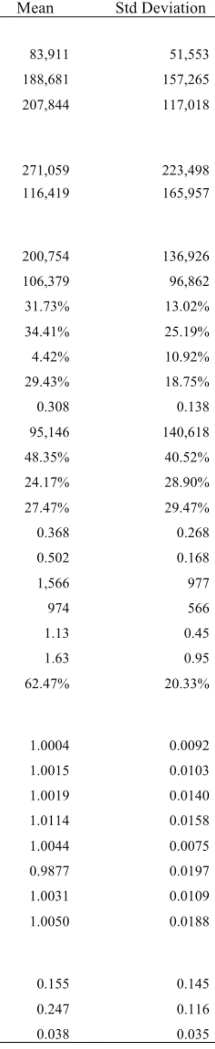
Summary statistics for the sample of farms are presented in Table 1. For a farm to be included in the analysis, continuous whole-farm data had to be available from 1979-2008. There were 135 Kansas Farm Management Association (KFMA) farms with the required data. For more infor-mation on the variables available in the KFMA databank and variable definitions see Langemeier (2010).
Input and output indices were computed for each farm and year by dividing income and expense items by price indices. The inputs used in the analysis were labor, purchased inputs, and capital. Labor included hired labor as well as family and operator labor. Purchased inputs in-cluded seed and other crop expense, fertilizer and lime, herbicide and insecticide, feed purchased, veterinarian expenses, fuel and utilities, and mis-cellaneous expenses. Capital included repairs, machine hire, cash interest, cash farm rent, prop-erty taxes, general farm insurance, depreciation, and an interest charge on owned equity. The out-puts used in the analysis were crop and livestock. Additional regression analysis broke crop income down into feed grain, small grain, hay and forage, and oilseed income; and livestock income into beef, dairy, and swine income.
The average value of farm production over the 30-year period was $200,754. Crop income and
livestock income were $106,379 and $95,166, respectively. Average total acres and crop acres were 1,566 acres and 974 acres, respectively. On average, approximately 62 percent of farmers’ time was spent on crop production. The largest source of crop income was small grains, which was comprised almost exclusively of wheat. Beef income was by far the largest source of livestock income. The average profit margin and asset turnover ratios were 0.155 and 0.247, respectively. The average crop, livestock, and aggregate crop and livestock diversification indices were 0.308, 0.368, and 0.502, respectively. These indices were computed using standard Herfindahl indices by summing the squared share of income from each enterprise or group of enterprises. For ex-ample, the crop diversification index was calcu-lated using the shares of crop income coming from each crop enterprise. A value of 1 would indicate that all income was coming from one source. Alternatively, a smaller value would indi-cate that the farm was more diversified and in-come was coming from several enterprises.
Results
The average MPI over the 30-year period was 1.0050, resulting in an average annual change in productivity of 0.50 percent. The highest average change was 6.46 percent and the lowest average change was -7.99 percent. Technical change aver-aged 0.31 percent per year, and efficiency change averaged 0.19 percent per year.
Table 2 provides a summary of the differences in farm characteristics, productivity indices, and financial ratios by categories defined using the MPI. Farms in the top third had an average MPI of at least 1.0159, and farms in the bottom third had an average MPI of less than 0.9963. The average annual productivity increase for the top 45 farms was 2.39 percent, while the average annual productivity decrease for the bottom 45 farms was 1.46 percent. If the farms in the top group continued to have an annual productivity increase of 2.39 percent compared to the average of 0.50 percent, with inputs remaining the same, outputs would increase by 27 percent for the top group and only 5 percent for the average farm over a 10-year period.
The first 10 years of the sample period (1979-1988) saw the largest differences between the top and bottom farms in terms of MPI. The average
Table 1. Summary Statistics for Sample of Kansas Farms, 1979-2008
Mean Std Deviation
Inputs
Labor Index 83,911 51,553
Purchased Input Index 188,681 157,265
Capital Index 207,844 117,018
Outputs
Crop Index 271,059 223,498
Livestock Index 116,419 165,957
Farm Characteristics
Value of Farm Production (VFP) 200,754 136,926
Crop Farm Income (CFI) 106,379 96,862
Percent of CFI from Feed Grain Income (corn and grain sorghum) 31.73% 13.02% Percent of CFI from Small Grain Income (primarily wheat) 34.41% 25.19%
Percent of CFI from Hay and Forage Income 4.42% 10.92%
Percent of CFI from Oilseed Income (soybeans and sunflowers) 29.43% 18.75%
Crop Diversification Index 0.308 0.138
Livestock Farm Income (LFI) 95,146 140,618
Percent of LFI from Beef Income 48.35% 40.52%
Percent of LFI from Dairy Income 24.17% 28.90%
Percent of LFI from Swine Income 27.47% 29.47%
Livestock Diversification Index 0.368 0.268
Crop and Livestock Aggregate Diversification Index 0.502 0.168
Total Acres 1,566 977
Total Crop Acres 974 566
Number of Operators 1.13 0.45
Number of Workers (includes hired, family, and operator labor) 1.63 0.95
Crop Labor Percentage 62.47% 20.33%
Productivity Indices
Pure Technical Efficiency Change (PTEC) 1.0004 0.0092
Scale Change (SCC) 1.0015 0.0103
Efficiency Change (EFFC) 1.0019 0.0140
Input Biased Technical Change (IBTECH) 1.0114 0.0158
Output Biased Technical Change (OBTECH) 1.0044 0.0075
Magnitude Component (MATECH) 0.9877 0.0197
Technical Change (TECH) 1.0031 0.0109
Malmquist Productivity Index (MPI) 1.0050 0.0188
Financial Efficiency Ratios
Profit Margin 0.155 0.145
Asset Turnover Ratio 0.247 0.116
Table 2. Farm Characteristics of Kansas Farms in the Bottom, Middle, and Top Thirds by Malmquist Productivity Indices, 1979-2008
Top 45
Farms 45 Farms Middle 45 Farms Bottom
Farm Characteristics
Value of Farm Production (VFP) 160,463a 184,044a 257,755b
Crop Farm Income (CFI) 78,915a 92,798a 147,422b
Percent of CFI from Feed Grain Income (corn and grain sorghum) 25.89%a 33.77%b 33.58%b
Percent of CFI from Small Grain Income (primarily wheat) 46.87%a 29.82%b 30.63%b
Percent of CFI from Hay and Forage Income 6.11%a 5.16%a 3.06%b
Percent of CFI from Oilseed Income (soybeans and sunflowers) 21.13%a 31.25%b 32.73%b
Crop Diversification Index 0.335a 0.303b 0.315b
Livestock Farm Income (LFI) 75,884a 91,857a 117,698a
Percent of LFI from Beef Income 61.40%a 44.57%a 42.89%a
Percent of LFI from Dairy Income 33.66%a 36.31%a 8.59%a
Percent of LFI from Swine Income 4.95%a 19.12%ab 48.52%b
Livestock Diversification Index 0.493a 0.367a 0.427a
Crop and Livestock Aggregate Diversification Index 0.500a 0.500b 0.506b
Total Acres 1743a 1417a 1539a
Total Crop Acres 964ab 834a 1124b
Number of Operators 1.07a 1.15a 1.18a
Number of Workers (includes hired, family, and operator labor) 1.48a 1.54a 1.87a
Crop Labor Percentage 63.88%a 57.93%a 65.60%a
Productivity Indices
Pure Technical Efficiency Change (PTEC) 0.9938a 1.0018b 1.0057c
Scale Change (SCC) 0.9957a 1.0025b 1.0064c
Efficiency Change (EFFC) 0.9895a 1.0042b 1.0121c
Input Biased Technical Change (IBTECH) 1.0106a 1.0127a 1.0109a
Output Biased Technical Change (OBTECH) 1.0055a 1.0039a 1.0039a
Magnitude Component (MATECH) 0.9803a 0.9855a 0.9971b
Technical Change (TECH) 0.9959a 1.0015b 1.0118c
Malmquist Productivity Index (MPI) 0.9854a 1.0057b 1.0239c
Financial Efficiency Ratios
Profit Margin 0.135a 0.131a 0.184b
Asset Turnover Ratio 0.215a 0.258b 0.264b
Rate of Return on Investment 0.029a 0.034a 0.048b
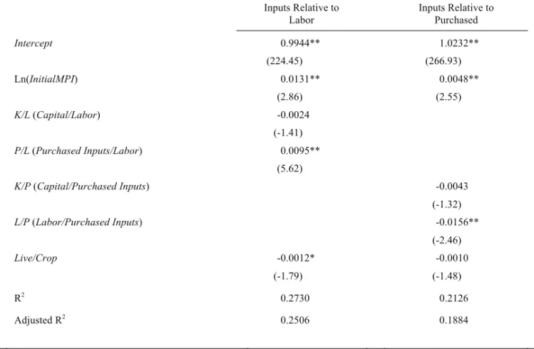
Table 3. Impact of Initial Malmquist Productivity Index, Relative Factor Intensities, and Output Ratio on Malmquist Productivity Index
Inputs Relative to Labor Inputs Relative to Purchased Intercept 0.9944** 1.0232** (224.45) (266.93) Ln(InitialMPI) 0.0131** 0.0048** (2.86) (2.55) K/L (Capital/Labor) -0.0024 (-1.41) P/L (Purchased Inputs/Labor) 0.0095** (5.62) K/P (Capital/Purchased Inputs) -0.0043 (-1.32) L/P (Labor/Purchased Inputs) -0.0156** (-2.46) Live/Crop -0.0012* -0.0010 (-1.79) (-1.48) R2 0.2730 0.2126 Adjusted R2 0.2506 0.1884
Note: The numbers in parentheses are the t-values. Double asterisk (**) indicates significance at the 5 percent level and single asterisk (*) indicates significance at the 10 percent level.
annual productivity increase for the top farms was 2.18 percent, and the average annual productivity decrease for the bottom farms was 2.49 percent during this time period. The second 10 years (1989-1998) resulted in the highest productivity increases for both the top and bottom farms, with average annual productivity increases of 6.49 per-cent for the top group and 3.68 perper-cent for the bottom group. The last 10-year period (1999-2008) resulted in negative growth for both groups. Average annual productivity decreased 1.75 per-cent for the top group and decreased 5.80 perper-cent for the bottom group during this time period. The productivity decrease during the last 10-year period may be due to the fact that the av-erage age of the primary farm operator was in-creasing. On average, the primary farm operator in the sample was 45 years old during the first 10 years of the sample period and 62 years old dur-ing the last 10-year period. Only 18 of the 135 farms had a change in the primary operator dur-ing the sample period, and most of the changes
occurred in the first 20 years of the sample. The efficiency change component of MPI was greater than 1 for the last ten years, but the technical change component was less than 1 for the last 10 years of the sample period. Thus, the productivity decrease is partially attributable to the fact that the farmers were not keeping up with tech-nological advances. The efficiency of the farmers was continuing to increase, but without an in-crease in technology adoption, change in produc-tivity was regressive. These results are consistent with Tauer and Lordkipanidze (2000). As farmers age, their productivity first increases and then decreases.
Comparing farm characteristics, the farms in the top productivity group were larger in terms of value of farm production, crop farm income, and livestock farm income. The average value of farm production for the 45 farms in the top group was $257,755 and for the 45 farms in the bottom group was $160,463. The number of operators was not significantly different for the top and
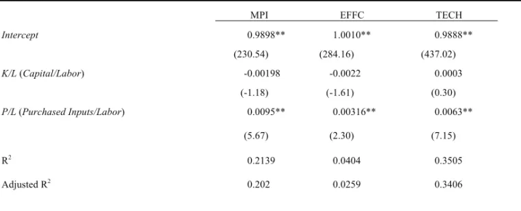
Table 4. Impact of Factor Ratios on Malmquist Productivity Index, Efficiency Change, and Technical Change
MPI EFFC TECH
Intercept 0.9898** 1.0010** 0.9888** (230.54) (284.16) (437.02) K/L (Capital/Labor) -0.00198 -0.0022 0.0003 (-1.18) (-1.61) (0.30) P/L (Purchased Inputs/Labor) 0.0095** 0.00316** 0.0063** (5.67) (2.30) (7.15) R2 0.2139 0.0404 0.3505 Adjusted R2 0.202 0.0259 0.3406
Note: The numbers in parentheses are the t-values. Double asterisk (**) indicates significance at the 5 percent level and asterisk (*) indicates significance at the 10 percent level.
bottom group, but the size of the farms in terms of value of farm production was significantly dif-ferent, indicating that the top 45 farms were using labor more efficiently. On average, the farms in the top third had more farm income coming from oilseeds and feed grains and less coming from small grains and hay and forage, as compared to the farms in the bottom third. In terms of income from livestock sources, the farms in the top third had, on average, more income coming from swine compared to the farms in the bottom third. Struc-tural changes in the swine industry have led to substantial increases in productivity, with total factor productivity increasing at an average an-nual rate of 5.2 percent from 1992 to 2004 for the region including Kansas (Key, McBride, and Mosheim 2008).
The farms in the top third had significantly higher profit margins, asset turnover, and rate of return on investment ratios. It is important to note that the rate of return on investment ratio did not include capital gains on land. The top third also had significantly higher values for pure techni- cal efficiency change, scale change, efficiency change, the magnitude component, technical change, and MPI. The bottom third had negative average growth in all components of MPI except for input biased technical change and output biased technical change. For all productivity groups, input biased technical change was larger than output biased technical change, indicating
that technological change is more biased on the input side than the output side. This is consistent with the results of Managi and Karemera (2004) for U.S. agriculture from 1960 to 1996.
The regression results pertaining to convergence indicated a significant positive relationship be-tween the average MPI and the log of the initial MPI; thus, the sample of farms experienced di-vergence (Table 3). In other words, there has not been a tendency for the farms with an initial lower productivity index to catch up to the productivity growth rate of the top farms in the sample. The coefficient for the purchased inputs to labor ratio was positive and significant at the 5 percent significance level, indicating that as pur-chased inputs grow relative to labor, the average MPI increases. This indicates that the farms with more intensive operations had higher productivity growth. The coefficient for the livestock to crop ratio was negative and significant at the 10 per-cent significance level, indicating that as livestock outputs increase relative to crop outputs there is a decrease in the average MPI. This indicates that crop and livestock production are not as comple-mentary as in the past. For most operations, an increase in crop outputs would result in increased productivity. Additionally, Table 3 presents the results of equation (2) using the capital to pur-chased inputs ratio and labor to purpur-chased inputs ratio to determine if the farms were input using or saving with respect to purchased inputs. The
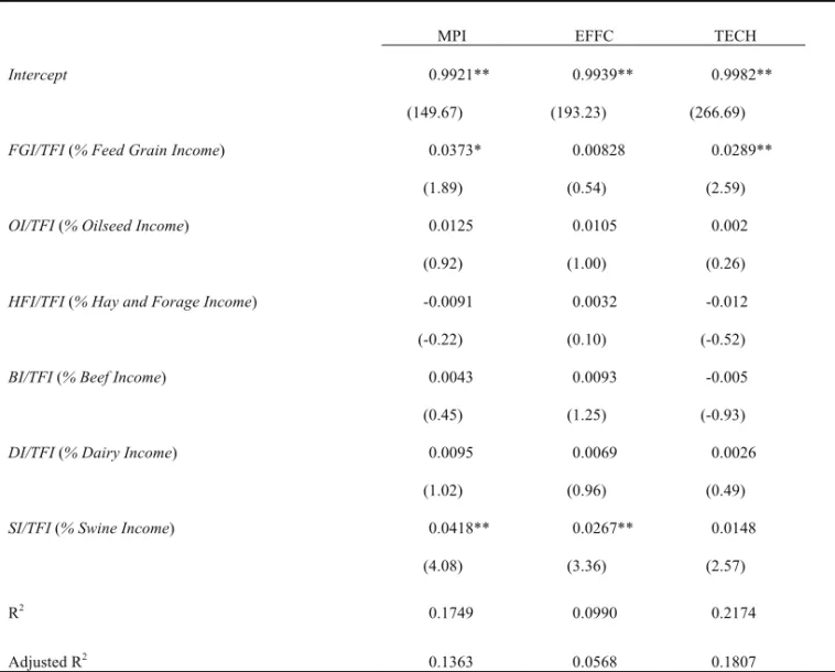
Table 5. Impact of Income Shares on Malmquist Productivity Index, Efficiency Change, and Technical Change
MPI EFFC TECH
Intercept 0.9921** 0.9939** 0.9982**
(149.67) (193.23) (266.69)
FGI/TFI (% Feed Grain Income) 0.0373* 0.00828 0.0289**
(1.89) (0.54) (2.59)
OI/TFI (% Oilseed Income) 0.0125 0.0105 0.002
(0.92) (1.00) (0.26)
HFI/TFI (% Hay and Forage Income) -0.0091 0.0032 -0.012
(-0.22) (0.10) (-0.52)
BI/TFI (% Beef Income) 0.0043 0.0093 -0.005
(0.45) (1.25) (-0.93)
DI/TFI (% Dairy Income) 0.0095 0.0069 0.0026
(1.02) (0.96) (0.49)
SI/TFI (% Swine Income) 0.0418** 0.0267** 0.0148
(4.08) (3.36) (2.57)
R2 0.1749 0.0990 0.2174
Adjusted R2 0.1363 0.0568 0.1807
Note: The numbers in parentheses are the t-values. Double asterisk (**) indicates significance at the 5 percent level and asterisk (*) indicates significance at the 10 percent level. Small grain income was the default for comparison purposes.
results were consistent across both specifications of equation (2).
The results in Table 2 for IBTECH and OBTECH, as well as the results with respect to input and output ratios, suggest that input and out-put bias exist. To further explore inout-put and outout-put bias, Table 4 examines the relationship between MPI, EFFC, and TECH, and input ratios; and Table 5 explores the relationship between MPI, EFFC, and TECH, and income shares. The pur-chased inputs to labor ratio had a positive and significant impact on MPI, EFFC, and TECH (Table 4), indicating that an increase in purchased inputs compared to labor resulted in a movement towards the production frontier and a shift in the production frontier. The capital to labor ratio did not have a significant impact on MPI, EFFC, and
TECH. The results in Tables 3 and 4 thus suggest that technical change was biased towards pur-chased inputs.
Regression analysis was used in Table 5 to explore the relationship between MPI, EFFC, and TECH, and income shares. Small grain income was removed from the regressions to prevent the independent variables from summing to unity. This variable was chosen because it represented the largest average source of income for the farms. An increase in swine income had a positive and significant effect on MPI and EFFC. An increase in feed grain income had a positive and signi-ficant effect on MPI and TECH. The results with respect to TECH in Table 5 suggest that technical change was biased towards feed grains and away from small grains. This result is consistent with
trends in feed grain and wheat acreage in Kansas over the last 35 years (Langemeier 2009).
Summary and Conclusions
This study used 30 years of continuous data for 135 farms in Kansas to determine whether or not the farms were experiencing convergence or di-vergence and to explore changes in productivity at the farm level. Malmquist productivity indices were calculated for each farm. These indices were used to determine whether there was productivity convergence or divergence in Kansas farms. The results showed that there was significant diver-gence among the farms. Thus, farms did not tend to catch up to the same growth rates of produc-tivity as the top farms in the sample.
This study adds to the previous literature that has found divergence at the state or country level. It is reasonable to assume that divergence would be found across states that vary in their land characteristics and outputs produced, but it could be argued that on a farm level in a particular state you would expect to find convergence if the farms were attempting to be competitive in the industry. Because it was found that the farms in this sample experienced divergence, the char-acteristics of the farms were examined to help determine what was driving the high productivity growth of the top farms.
The average annual productivity growth over the sample period, 1979-2008, was 0.50 percent. The average growth for the top 45 farms based on MPI was 2.39 percent and the average produc-tivity decrease was 1.46 percent for the bottom 45 farms. On average, both groups of farms had productivity increases from 1989-1998 and pro-ductivity decreases from 1999-2008.
The top farms, based on MPI, were larger in terms of value of farm production, crop farm in-come, and livestock farm income. They also had significantly higher efficiency change and techni-cal change indices and financial efficiency ratios. The top group received a larger percentage of their income from oilseeds, feed grains, and swine than the other farms, on average, and relatively less of their income from small grains.
A closer examination of the top six farms based on MPI reveals that you cannot make recom-mendations solely based on characteristics of the top one-third productivity group. As noted above, there was a tendency for the top 45 farms to be
larger and receive relatively more income from oilseeds, feed grains, and swine. However, it is important to note that the top six farms were quite different in terms of size and farm type. Only two of the top six farms were above average in size, measured using value of farm production. Three of the top six farms were primarily crop with the largest portion of income coming from small grains or oilseeds. The three top farms that were primarily livestock produced swine. The differ-ences among these farms indicate it is important to examine the productivity and efficiency of farms on a regular basis and for the individual farms to benchmark or regularly examine their competitive position.
This study lends support to the argument that productivity tends to increase with age to a certain point and then decrease. On average, annual pro-ductivity grew for the first 20 years of this study and then decreased for the last 10 years. An im-plication evolving from this is as farm operators age and transition out of farming, there is likely to be more consolidation of farms.
The fact that the farms are not experiencing convergence is consistent with the notion of com-petitive advantage and the fact that the farms in the top third are taking advantage of unique re-sources or characteristics to allow them to consis-tently outperform their peers (Porter 1998, Barney and Clark 2007). The identification of these unique resources is an important avenue for future research.
References
Ariyaratne, C.B., A.M. Featherstone, and M.R. Langemeier. 2006. “What Determines Productivity Growth of Agricultural Cooperatives?” Journal of Agricultural and Applied Economics 38(1): 47-59.
Ball, V.E., C. Hallahan, and R. Nehring. 2004. “Convergence of Productivity: An Analysis of the Catch-up Hypothesis within a Panel of States.” American Journal of Agricultural Economics 86(5): 1315-1321.
Barney, J.B., and D.N. Clark. 2007. Resource-Based Theory: Creating and Sustaining Competitive Advantage. Oxford: Oxford University Press.
Barro, R.J., and X. Sala-i-Martin. 1991. “Convergence across States and Regions.” Brookings Papers on Economic Activity 1991(1): 107-158.
Barro, R.J., and X. Sala-i-Martin. 1992. “Convergence.” Journal of Political Economy 100(2): 223-251.
Clark, P., and M. Langemeier. 2007. “Productivity and Farm Size.” Selected paper presented at the 16th International
Farm Management Association Congress–UCC, Cork, Ireland.
Cochran, W.G., and G.M. Cox. 1992. Experimental Designs (2nd Edition). New York: John Wiley and Sons.
Coelli, T.J., and D.S.P. Rao. 2003. “Total Factor Productivity Growth in Agriculture: A Malmquist Index Analysis of 93 Countries, 1980-2000.” Working Paper Series No. 02/2003, Centre for Efficiency and Productivity Analysis, School of Economics, University of Queensland.
Coelli, T.J., D.S.P. Rao, C.J. O’Donnell, and G.E. Battese. 2005. An Introduction to Efficiency and Productivity Analysis (2nd Edition). New York: Springer.
Färe, R., and S. Grosskopf. 1996. Intertemporal Production Frontiers: With Dynamic DEA. Boston: Kluwer Academic Publishers.
Färe, R., S. Grosskopf, M. Norris, and Z. Zhang. 1994. “Productivity Growth, Technical Progress, and Efficiency Change in Industrialized Countries.” The American Eco-nomic Review 84(1): 66-83.
Fuglie, K.O., J.M. MacDonald, and E. Ball. 2007. “Produc-tivity Growth in U.S. Agriculture.” Economic Brief No. 9, USDA/Economic Research Service, Washington, D.C. Islam, N. 2003. “What Have We Learnt from the Convergence
Debate?” Journal of Economic Surveys 17(3): 309-62. Key, N., W. McBride, and R. Mosheim. 2008.
“Decom-position of Total Factor Productivity Change in the U.S. Hog Industry.” Journal of Agricultural and Applied Economics 40(1): 137-149.
Langemeier, M.R. 2010. "Kansas Farm Management SAS Data Bank Documentation." Staff Paper No. 11-01, Depart-ment of Agricultural Economics, Kansas State University, Manhattan, Kansas.
Langemeier, M. 2009. “Relative Efficiency of Kansas Wheat Farms.” Paper presented at the 2009 Risk and Profit Con-ference, Department of Agricultural Economics, Kansas State University, Manhattan, Kansas.
Managi, S., and D. Karemera. 2004. “Input and Output Biased Technological Change in U.S. Agriculture.” Applied Eco-nomics Letters 11(5): 283-286.
Olson, K., and L. Vu. 2009. “Productivity Growth, Technical Efficiency, and Technical Change on Minnesota Farms.” Selected paper presented at the 2009 Agricultural and Applied Economics Association Annual Meeting, Milwaukee, WI.
Porter, M.E. 1998. On Competition. Boston: Harvard Business School Publishing.
Sala-i-Martin, X. 1996. “The Classical Approach to Con-vergence Analysis.” The Economic Journal 106(497): 1019-1036.
SAS Institute. 2005. SAS/STAT User's Guide, Version 9.1. Cary, NC: SAS Institute.
Tauer, L.W., and N. Lordkipanidze. 2000. “Farmer Efficiency and Technology Use with Age.” Agricultural and Resource Economics Review 29(1): 24-31.