Automatic image colorization

Treball final de grau

GRAU D’ENGINYERIA INFORMÀTICA

Facultat de Matemàtiques i Informàtica

Universitat de Barcelona

Automatic Image Colorization

Author: Guillem Pascual

Supervisor:

Dr. Santi Seguí

Completed in: Departament de

Matemàtiques

i Informàtica

Abstract

Colorizing is the act of giving color to grayscale images. A convolutional-neural-network-based method to colorize images without human interaction is presented in this project. Various frameworks, architectures, color spaces and approximations are explored to obtain the final model, capable of correctly restoring the original color of photographies without any further information than the image itself.

The principal aim of this project is to propose an idempotent architecture that could be trained with all kinds of images and yet produce good results. To demonstrate how the process works and show the obtained results, three categories of images will be used along this project: synthetic images representing numbers, landscape images and human faces.

Resum

Coloritzar consisteix en dotar de color a imatges originalment en escala de grisos. En aquest treball es presenta un mètode basat en xarxes neuronals convolucionals per coloritzar imatges sense cap interacció humana. Diferents frameworks, arquitectures, espais de color i aproximacions s’exploraran per obtenir el model final, capaç de restau-rar de forma adequada el color original de fotografies, sense cap altre informació que la mateixa imatge.

L’objectiu final d’aquest projecte es presentar una arquitectura idempotent que pu-gui ser entrenada amb qualsevol tipus d’imatge i produir bons resultats. Per demostrar que el procés funciona i mostrar els resultats obtinguts, es faran servir tres categori-es diferents d’imatgcategori-es: imatgcategori-es sintètiqucategori-es que reprcategori-esenten números, paisatgcategori-es i carcategori-es humanes.

Acknowledgements

First of all, I would like to express my gratitude to Dr. Santi Seguí. Not only for his incommensurable support and assistance throughout this research project, but also for his guidance all along this course. This project would not be the same without him.

I would also like to thank my whole family, for giving me the opportunity to study this degree and for helping me reach thus far. I am particularly grateful to Aida Montserrat, for her patience, her reviews and critiques to improve this project and for constantly encouraging me and pushing me further.

Lastly, I would also like to acknowledge all Universitat de Barcelona’s professors, for teaching me the necessary concepts to become who I am, and all my friends and classmates who have accompanied me during this trajectory.

Contents

1 Introduction 1

1.1 Context . . . 1

1.2 Motivation and Objectives . . . 1

1.3 Memory organization . . . 2

2 State of the Art 4 3 Artificial Neural Networks 5 3.1 What are they? . . . 5

3.2 Activation Functions . . . 8

3.2.1 Linear . . . 8

3.2.2 Binary threshold . . . 9

3.2.3 Sigmoid . . . 9

3.2.4 Hyperbolic tangent . . . 9

3.2.5 Rectified Linear Units . . . 10

3.2.6 Other activation functions . . . 10

3.3 Layers . . . 10 3.3.1 Fully Connected . . . 11 3.3.2 Dropout . . . 11 3.3.3 Convolution . . . 12 3.3.4 Pooling . . . 13 3.3.5 Batch Normalization . . . 14 3.3.6 Summation . . . 14 3.3.7 Other layers . . . 15 3.4 Learning algorithm . . . 15 4 Architecture 19 4.1 Method 1: Convolutional and fully connected layers . . . 19

4.2 Method 2: Fully convolutional networks . . . 20

4.2.2 Residual Networks . . . 21 4.2.3 Color space . . . 23 4.2.4 Final architecture . . . 24 5 Implementation 27 5.1 Frameworks . . . 27 5.1.1 Caffe . . . 27 5.1.2 Tensorflow . . . 27 5.2 Network implementation . . . 28 5.2.1 Optimizer . . . 28 5.2.2 Number of parameters . . . 28 5.2.3 Tensorflow specific . . . 29 5.2.4 Visualization . . . 31 5.3 Online website . . . 34 5.3.1 Backend . . . 35 5.3.2 Frontend . . . 36 5.3.3 Communication . . . 36 6 Results 38 6.1 Measure of quality . . . 38 6.2 Datasets . . . 39 6.2.1 Synthetic data . . . 39 6.2.2 Landscapes . . . 41 6.2.3 Faces . . . 46 7 Conclusions 51 7.1 Research conclusions . . . 51 7.2 Future work . . . 52 References 54

1 Introduction

1.1 Context

The main aim of this project is to contribute to the research of the artificial networks field, and specifically to convolutional neural networks. It will be focused on applications of this machine learning sub-field, making special emphasis on its capacity to learn by themselves. Image colorization, a technique based on coloring an image which is only available in grayscale, has existed from long before. However, most works until recently had to be done either by using Photoshop or such programs or even by completely painting the image by hand. That means the user criteria and experience came to the scene, being perhaps the most important source of information. This process, when done manually, might take up to hours or even days to accomplish, while the solution we seek for should only delay a few milliseconds until it produced a colored image.

Artificial neural networks are perfect for this task. Their training time might be high, but then testing or producing results is done in a matter of milliseconds. More important even, they have the capacity to learn all alone. All the subfields of artificial neural networks are quickly evolving, within a span of fewer than 10 years we have seen innumerable new techniques that overwhelm the already existing. Convolutional neural networks, the main architecture used in this project, are no exception [1].

The Treball de Fi de Grau (TFG) makes a particular stress on what has been taught in the subject ”Aprenentatge automàtic i minèria de dades”, as in it applies much of the concepts taught there, from regressions to cross-validation. It also has a relation with ”Taller de nous usos de la informàtica”, but it rather expands the knowledge taught there.

1.2 Motivation and Objectives

Neural networks are not only, as said above, constantly updating but considered to be state of the art in many research fields. The aim of this project is to further research on them and propose new cases of use along with techniques that might outperform existing meth-ods. When this project was started no other known implementations of colorization through convolutional neural network existed, thus it was, aside from research, a new method for col-orization automatization. This work should serve as scientific research, personal publication and final project.

As said, other methods exist that color images, but they require the user’s attention. My method aims to be completely user agnostic, in the sense that no action will ever be required from the user.

It must also be fast, within seconds the image should be colored and made available to the user. All existing implementations now either require a huge amount of previous time to model a feature space [2] or a vast number of examples like the grayscale image we want to colorize [3, 4]. This method should require neither of those, only the input image will be used, without needing hand-crafted features nor more examples.

All results should faithfully represent the reality. For example, skies should be colored blue and grass should be green. The algorithm must be consistent with the regions, as in all the grass should be painted the same color while preserving its texture and shape.

This project also takes the user into consideration. Aside from giving easy to use methods on the Python implementation, it will provide an intuitive and easy to navigate online website. The user should be able to simply select an image or drag it into the website for it to be colorized, thus making it not only fast and autonomous but accessible without any programming knowledge.

1.3

Memory organization

The structure followed in this project goes bottom-up, it first explains the inherent concepts in artificial neural networks and expands them until all the information necessary for understanding the implemented model has been taught. It is organized as follows:

1. State of the art: Related work with this project. Previous works and current imple-mentations considered to be performing best at the moment of writing this memory are introduced. A brief explanation of other methods and shallow comparisons are done.

2. Artificial Neural Networks: Artificial Neural Networks (ANN) have not been cov-ered in any course of the degree in Computer Science at the Universitat de Barcelona, thus a previous research had to be done. This section will cover the background in-formation required to develop this project. It aims at explaining what an ANN is and further proceed into explaining Convolutional Neural Networks (CNN).

This chapter covers the basic structures of the ANN, as well as the most important types of activations and layers. Backpropagation and gradient descend, the basic methods used in deep learning to train networks, will also be explained

3. Architecture: This section proposes architectures which are presumed to be able to address the colorization problem. They will be discussed and detailed, explaining the reasoning behind each choice and how each decision was taken.

4. Implementation: While the last section introduced the architecture used, this one will center on how they were particularly implemented. It will not only explain the frameworks used, Caffe and Tensorflow, but also enter into details on which optimizer was chosen and which hyperparameters where used and how were they found.

The developed website will also be detailed in this section, explaining the used tech-nologies: Python for the webserver and a combination of HTML/CSS/JS/AJAX for the client rendering and communication.

5. Results: Practical examples and discussion on the obtained results. The implemented architectures will be tested and the resulting images will be examined, both qualita-tively and quantitaqualita-tively, to elaborate on the network performance. It will also be noted some alternative modifications done to the network to attempt to improve it. 6. Conclusion: It will be written if the proposed objectives has been met or not. Cases

of good and bad performance will also be analyzed and conclusions will be extracted from them.

Some discussion on how to improve the current work and some future ideas will also be mentioned.

2

State of the Art

This section does an overview on some existing and just released methods which also address the colorization problem. They will be mentioned and briefly explained to put this project into perspective and better contextualize it.

As mentioned in the introduction, colorization is not a new problem. Some methods [2, 3, 4] already exist that attempt to solve it. They, however, require a huge previous effort from the user.

The first method to successfully remove all required user intervention, by using convo-lutional neural networks, appeared on January 2016 [5]. It uses a pretrained VGG Network [6], a neural network designed to classify images among 1.000 different classes using the Imagenet dataset [7], as a mean of initialization. To perform colorization it takes concepts from the Residual Networks [8], which will be explained in detail in the Architecture section. The images used to train, and also to test, are taken from this same Imagenet dataset and the results showed good performance. Its main interest is, as said, being totally unattended while producing realistic images. It has been widely explored and used, for example, to perform colorization on whole videos1_{. It even surprisingly manages to be consistent along} consequent frames, which is not trivial.

Some precedents exist, for example Z. Cheng’s Deep Colorization[9]. Unlike the first method, their method requires both crafting features and manually labelling the images so that a semantic segmentation is first done. Moreover, for their method to work a final post-processing has to be done to reduce the artefacts which result from the patch-based approach they take. This would not fit in the previous established objectives of not requiring user intervention and being fast, but it is still worth mentioning as the results obtained are amongst the best ones.

Some other recent methods [10, 11] produce much better results on the positive examples. On the other hand, they tend to miss-classify pixels and produce inconsistent results. Some erratic behaviour has been observed where the network attempt to paint outside of the textures and boundaries. Both, however, produce much more saturated results than the networks above, a problem we will introduce later in this document and fully explain and reason about.

This project will also use techniques considered state of the art, as it parts from [5] to construct a more complex method based on completely different datasets and explores beyond the original architecture.

1_{Colorizing Black&White Movies with Neural Networks: https://www.youtube.com/watch?v=}

3 Artificial Neural Networks

3.1 What are they?

A first, correct, definition of ANN is a computational model inspired by biological neural networks used to approximate functions that are not known a priori. They imitate the behaviour of neurons, but using a simplified model where only the electrical signal is taken into account and not the chemical processes.

Figure 1: Simplified biological model of a neuron

Image by Virtual Laboratory of Artificial Intelligence, Agh University

Take for example the neuron in Figure 1, one single neuron will receive information from a wide number of neurons through its dendrites. Further on, the synapses will decide whether that input will stimulate or inhibit the neuron activity. For each pair of dendrite and synapse, the result will be multiplied and summed with the others. If the neuron gets activated, because the signal has reached a high enough value, it will send a signal through its axon. Otherwise, it will remain silent (on the electrical perspective, it will send a 0V signal, whether elsewhere it would send a positive or negative voltage).

This biological simplification can easily be converted into a mathematical model, see Figure 2. The dendrites are now the input variable⃗x, which gets multiplied by a set of weights⃗w, the synapses. Two more concepts are also introduced, a function which collects all the products (which usually is the summation, but could also be the product), calledf(x) and the activation functiong(x). The whole operation could now be described in terms of:

Figure 2: Mathematical model of the biological neuron

Figure 2 also illustrates the simplest and first neuron that was implemented, called the McCulloch-Pitts neuron [12]. From Equation 1, and considering this neuron uses the binary threshold as activation, we have:

g(x) = {

1, ifx >0

0, otherwise (2)

f(x) =

∑

The McCulloh-Pitts neuron, all by itself, is capable of implementing simple lineal separa-ble prosepara-blems, such as the AND and OR functions, but fails to fit any non-lineally separasepara-ble model. Such limitation, as will be seen, can be overcame by building larger networks (Fig-ure 3) and appropriately choosing its layers and activation functions. A layer, indeed, is nothing else but a set of neurons put together, each with its connection (weight) to one or more neurons.

From this we can derive a more specialized definition, a neuronal network must:

1. Contain a set of adaptive weights which can be tuned by a learning algorithm (which will be further discussed in the next sections)

2. Be able to approximate non-lineal functions of their inputs, to be able to solve more complex problems

When creating an artificial neural network, we create networks of neurons. Each block of those networks is called a Layer, and depending on how we connect it with the previous

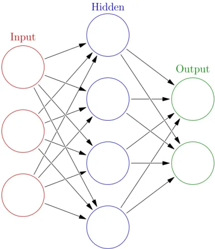
Figure 3: Artificial Neural Network: A Network of McCulloch-Pitts neurons

layer it receives one name or another. For example, on Figure 3 we would have 3 layers: the input layer, one hidden layer and the output one. A network is usually considered to be

deepwhen 2 or more hidden layers are used. Taking a closer look, the hidden layer consists of 4 neurons which are fully connected by the previous layer and fully connected to the next one. The termfully connected is explained in the Layers sections below.

We can also differentiate amongst some basic types of networks (although much more exist) depending on how we connect them:

1. Feedforward neural network: Layers are only connected in a forward way, there are not any connections between neurons in the same layer nor it can have connections to previous layers. The network is, then, assembled into a Directed Acyclic Graph (DAG).

2. Convolutional neural network: It is a specialization of the feedforward network but using convolutional layers (explained below) and retaining the original shape of the

input along the process.

3. Recurrent neural network: This type of network allows connections with previous layers and amongst itself, simulating a short term memory.

3.2

Activation Functions

Activations are a fundamental part of neural networks, as for them to be able to approx-imate any function, we must allow the network to calculate non-linearities. This section discusses the different types we may use.

The first thing to take into account is that the learning algorithm will use the derivative of all layers and activation functions to compute the error on the prediction done by the network, which implies that a requirement for any activation function is to be differentiable.

(a) Linear (b) Binary threshold (c) Sigmoid

(d) Hyperbolic Tangent _{(e) Rectified Linear Unit}

Figure 4: Activation functions

3.2.1 Linear

The linear activation is the most basic and, as it name implies, it does not perform any non-linearity (Figure 4a)

Its mathematical formula is:

3.2.2 Binary threshold

We have already seen this activation function as part of the McCulloch-Pitts neuron (Equation 2), its graphical representation is shown in Figure 4b.

3.2.3 Sigmoid

This function maps an input value into the range[0, 1](Figure 4c) by using the formula below:

g(x) = 1

1+e−x (3)

The sigmoid activation has been widely used successfully due to its easy and fast deriva-tive. Knowing that(ex)′=x′ex, we can simply derive it with:

g′(x) =g(x)(1−g(x))

That means the same values obtained by the activation of the function, g(x), can be reused when computing the derivative. This makes the function blazing fast by caching the activation results and reusing them later.

3.2.4 Hyperbolic tangent

This function maps an input value into the range[−1, 1](Figure 4d) by using the formula below:

g(x) =tanh(x) (4)

Alike the sigmoid function, the derivative of the tanh function can reuse the values from the activation itself:

g′(x) =1−g2(x)

Caching the activation values will, again, make this function faster. The main difference with the sigmoid activation relies on having a higher slope and a wider range.

3.2.5 Rectified Linear Units

Rectified Linear Units [13] (or ReLU for short) are an improved version of the linear activation which are shown to dramatically improve the performance of a network. Their most important feature is improving the gradient stability (something that will be discussed further on the learning algorithm section), which makes the network able to be deeper and learn better features.

The activation is given by (Figure 4e):

g(x) = {

x, ifx>0

0, otherwise (5)

3.2.6 Other activation functions

Recent papers have shown some other activation functions to have equal or better per-formance. They will be briefly mentioned but no expanded because they are not being used during this project:

1. Leaky ReLU [14]: g(x) = { x, ifx>0 αx, otherwise Where al pha≈0.01

2. Exponential Linear Unit [15]:

g(x) = { x, ifx>0 α(ex−1), otherwise 3. Parametric ReLU [16]: g(x) = { x, ifx>0 αx, otherwise Whereαis a learnable parameter

3.3

Layers

Depending on how we connect the layer to the previous ones or even on the operation they perform, we might distinguish into a wide range of layers.

3.3.1 Fully Connected

This type of layer, which can also be called Dense layer, connects each neuron of the previous layer with each of the neurons this layer itself has. Therefore, if the previous layer hasn neurons and this one hasmneurons, the total number of connections done aren·m. Although we now talk in terms of connections, a much better term would be parameters or weights. If we recall Equation 1 and Figure 2, a neuron activation was defined as the dot product (summation of multiplication) on⃗x and a set of weights⃗w, the connections. Thus, from here on we will talk in terms of weights or parameters the neural network must learn to fit a function.

It is clear that the fully connected layer can not be huge, as its size would soon be bigger than the memory we have available. Supposing we work withfloat32data types, each weight would occupy a total of 4 bytes, which gives an allocation ofn·m·4bytes.

One associated problem with fully connected layers is also the overfitting of the training data. That is, a neural network composed solely of fully connected layers will tend to fit too much on the training data and lose the capacity to generalize on new data, which will make new predictions fail. This gets worst the bigger the fully connected layer is (the most neurons it has). Also, stacking too much layers of this type would produce overfit or make the gradients explode (go out of the data range).

3.3.2 Dropout

On the theme of preventing overfitting, the Dropout [17] comes to action. Its working principle is straightforward, some of the neurons in the layer are set to 0, so that their activation is inhibited. Those neurons are chosen at random from a fraction of the total neurons (from0.1to0.7usually).

Deactivating some neurons implies the other ones must be accordingly scaled, so as to preserve the gradient. It could be implemented by:

g(xi) = {

xi/(1−ratio), ifrndi>ratio

0, otherwise

Whererndi is a random value per neuron∈[0, 1]andratio is also a value∈[0, 1]. This effectively reduces the overfitting by allowing the network to not completely rely on each of the activations and rather look for general patterns.

3.3.3 Convolution

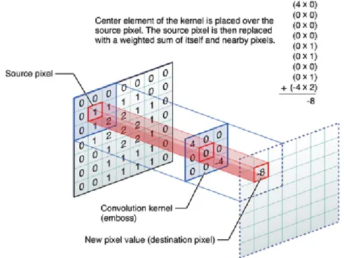
A convolution layer is a biologically inspired layer [18] which performs the operation it name implies, a convolution over the image. A convolution (Figure 5) is performed by sliding a kernel (a pattern) of sizek·p (usuallyk= p, where kand pare odd) over the image and computing the element-wise multiplication of its elements by the images on each pixel. The main advantage over the traditional convolutions is that features, or kernels, must not be hand-chosen, as the network learns the best features for its input.

Figure 5: Convolution of a 3x3 kernel on a reference image Image by Apple

Convolutions have a few advantages over fully connected layers:

1. When working with images, they:

(a) Preserve the spatial shape of the image along the forward and backward pass (b) Find textures on the image

(c) Find boundaries on the image

2. They greatly reduce the number of parameters of the network

The number of parameters of this layer is equal to the kernel’s size. We say this layer has shared weights because it applies the samek·p weights all over the image (it convolves

thek·p kernel), instead of having a weight per neuron/connection like the fully connected layer. We usually let this layer produce more than a single filter, thus having q different filters of size k·p, giving a total of q·k·p parameters. Also, it may have an input of r channels (activations) which must also be taken into account, giving the final formula of: r·q·k·pparameters.

This layer allows to tune the following hyperparameters:

1. Number of filters: The capacity of the layer, how many filters it will convolve on the image. The shallower the layer, the fewer filters we need as less information is available.

2. Kernel size: The size of the kernel(s) to be convolved. As with traditional convolu-tions, the bigger the filter, the bigger structures it will find.

3. Stride: The interval at which the filter is applied to the input, usually 1

4. Padding: The kernel needs k/2extra pixels on the image for it to output an image of the same size of the original. This is usually solved by adding a 0 padding to the original image. Some frameworks, like Tensorflow, abstract it to some predefined padding types (’same’ and ’valid’).

3.3.4 Pooling

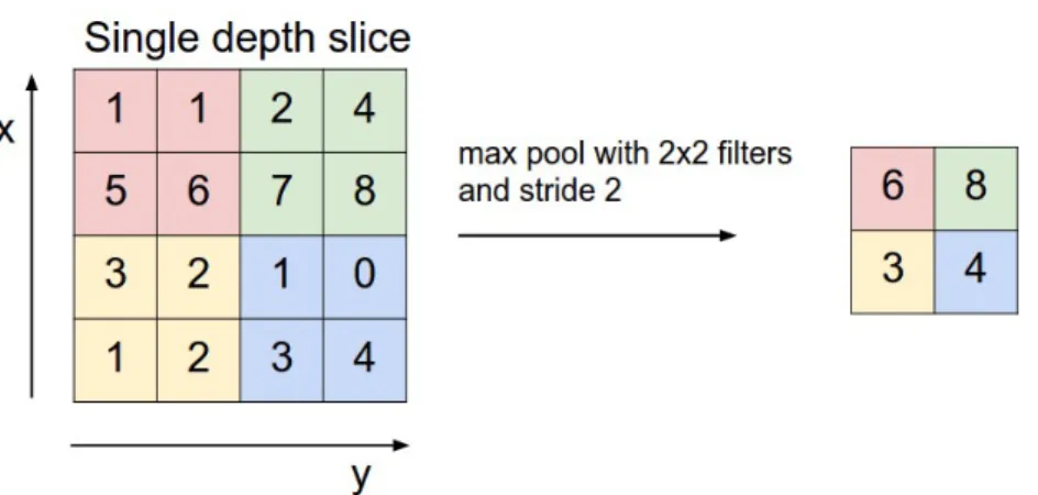
When working with CNNs the pooling layer is important because it allows performing non-linear downsampling of the original input image (Figure 6). This layer operates amongst regions of the input and performs an operation on them so that only one output is given. Specifically, it can compute the following operations:

1. Maximum: Over the region, output the maximum value found 2. Minimum: Over the region, output the minimum value found 3. Average: Output the average value of the region

4. Stochastic: Output a random value of the region

As with the convolutional layer, we can define the kernel size and stride. It is common in pooling operations to use a kernel size of 2x2 and a stride size equal to the size of the kernel, that is2 in this case (kin the general case).

When working with images the most used type is the maximum pooling, because it allows the network to be rotation invariant, in the sense that small changes will not affect it, as the overall intensity will be the same.

Figure 6: Pooling of a 2x2 kernel, stride 2, on a reference image Image by Stanford University

3.3.5 Batch Normalization

This layer normalizes its input by a moving average on the mean and standard deviation of the activations. It does, indeed, perform a standardization, the output has a 0 centered mean and standard deviation 1 [19]. It also biases and scales the values by two learnable parameters, also named bias and scale.

It has proven to be useful because it:

1. Stabilizes the gradient and solves exploding gradient problems 2. Helps reduce overfitting

3. Accelerates learning

4. Makes the learning rate influence more superficial, in the sense that finding a good learning rate becomes an easier task

It is being widely used and is thought to replace the local response normalization layer, which was used in conjunction to convolutions to normalize the activations, and even could deprecate the dropout layer.

3.3.6 Summation

This type of layer simply joins two other layers by performing the element-wise summa-tion of the activasumma-tion of both layers.

f(x1,x2) =x1+x2

It is commonly used in architectures like the residual networks, which will be detailed in section 4.2.2.

3.3.7 Other layers

In the field of Convolutional Neural Networks we also have the Local Response Normal-ization [20], which performs a neighbourhood value normalNormal-ization. More related to the field of feedforward networks we have the Highway Layer [21]. Some other layers not used in this project are the RNN related LSTM [22] and the GRU layer [23].

3.4 Learning algorithm

The algorithm to learn the weights or parameters of the network receives the name of

backward propagation of errors, abbreviated tobackpropagation. This method only works for supervised learning because it requires the target output to be known so that a loss function (error function) can be computed.

It is a generalization of the single-layer delta rule, updated to work with multi-layered networks. It requires to first forward2 the input through the network and then backprop-agate the errors from the output to the input, making each layer rectify its weights for a proportional part of its error. To correctly reduce the error we iteratively subtract a portion of the error, for example by using the gradient descent algorithm.

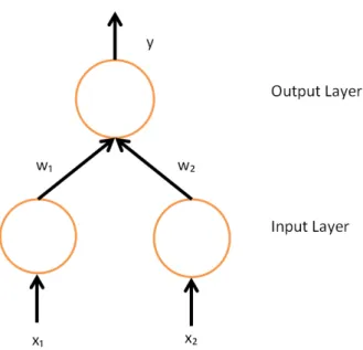
In the simpler case (Figure 7), a network with no hidden layers and only and input and output layer, we need to think of the network as an optimization problem, whose last layer outputs the error as:

E= 1 2(y−yˆ)

2

Whereyˆis the network prediction andythe target value3_{. Which, in the one-dimensional} space would produce a convex function whose representation can be seen in Figure 8.

We already know the error for the last layer and how to minimize it, by taking its derivative and moving into the direction that minimizes it:

2_{In neural networks feeding some input through the first layer and propagating it until the last is usually}

denoted as forward

3_{We include the term} 1

Figure 7: Network with no hidden layer, input fully connected to output

Figure 8: Euclidean error of a 1D function

E′ =y−yˆ (6)

In case of multi-layered networks, the contribution of the weightswij to this layerlayerj can be extrapolated by using the chain rule, that is:

δE δwij = δE δoutputj δoutputj δlayerj δlayerj δwij

However, we can see that δlayerj

δw_ij is the same as the output of the following layer. That means we have to start backpropagating the error from the last layer to the first one. We may also note that the derivative of an output with respect to its input is given by:

δoutputj δlayerj

= δg(x) δx

That is the derivative of the activation function with respect to its input. Thus, this connects with the statement made in Section 3.2, that all activation functions must be differentiable. If we suppose we are using the sigmoid functiong(x) = ₁₊1_e−x, then

δoutputj δlayerj

=g(x)(1−g(x))

Finally, the term _δoutputδE

j is straightforward in the output case of the output layer, where

we simply need to compute the derivative of the error (Equation 6). However, in case of a layer in the middle of the network, the error E is given by the accumulated error of the other layers, that is:

δE(outputj) δoutputj = δE(netj+1, ...,netj+k) δoutputj =

∑

Then, we can generalize this expression to:

δE δwij =σ_joutputi σj= δ E δoutputj δoutputj δlayerj = { (y−yˆ)g′(x), if jis output (_∑σ_iwji)g′(x), otherwise

Finally, we must update the network weights. It can be done by multiplying the error computed with a negated learning rateα. We change its sign because we want to find the minimum of the optimization problem. The termα, called learning rate, must be chosen so that the function converges fast but the steps are not too big:

∆wij =−α δE δwij

This last Equation 7 is called the Gradient Descend, which minimizes the error iteratively by taking steps. However, as easy as it looked with the convex function in Figure 8, a more realistic error function might be the one in Figure 9. This figure makes it clear that a small αwould make the minimization process get stuck in a local minimum. However, choosing a bigαwould make the function not converge and oscillate in the global minimum. Choosing the rightαis crucial for the network to work.

Figure 9: Real error function of a multi-layered network

Nowadays gradient descend is not used as is, but using the so called Stochastic Gradient Descend. The main reason behind this is that the first would require the whole dataset to be forwarded and backpropagated at once. Datasets usually consist of thousands or even millions of data, which makes this impossible. Input is then submitted either one-by-one or using mini-batches, small groups of data.

4 Architecture

In this section it is written an explanation on each of the tested architectures. It is explained how and why the final architecture was built and all the logical reasoning to come up with it.

4.1 Method 1: Convolutional and fully connected layers

Figure 10: 2xConvolutions of a 5x5 kernel without padding + 3x(1 fully connected layer of 1000 units + 1 fully connected layer of 784 units)

The initial version of the neural network was a combination of convolutional, pooling and fully connected layers (Figure 10). It can be said this first attempt is naive and simple, as it attempts to reconstruct the color with a small number of layers.

First, a common set of convolutional layers with ReLU activations is placed to allow the network to find textures. They are shared amongst the 3 resulting channels, RGB, as the textures will be the same independently on which channel will be used. The idea is to let these convolutional layers to find boundaries, textures and more complex representations

as they get deeper. A system like this one, which has a common set of layers first and then divides into more branches might be calledearly-fusion[24], while the opposed would be a late-fusion network. In the early-fussion approach, the features are considered to be dependent between them, which makes sense in our particular case.

Then, each channel of the RGB space is rebuilt separately by splitting the network into 3 different branches. Each of them contains a set of 2 fully connected layers with ReLU activations. For this to work, the last layer must have exactly the same size of the input image (for example, if working with 28x28images, it would be 28·28=784), because we must reshape them to the original size at the end.

The error, or loss, was computed as the sum of the euclidean distances between each of the resulting channels and the respective target channels.

In order to explain why an alternative architecture was used, we need to analyse this network from the point of view of the number of parameters. The network worked fine when an image of low resolution, for example28x28, was used. But when trying with bigger images of size256x256, the last layer had to be of 256·256=65536 neurons. That means it would require a total of65536·1000=65536000parameters only for the last layer. That exceeds the maximum size of an integer (215_{−1=32767) and is about 260MB of memory}

(65536000·sizeo f(f loat) = 65536000·4 ≈ 260MB), which makes it impractical for any

learning process to succeed.

It became clear that a network using fully connected layers would not be able to accom-plish the task due to memory constraints and computational power limits. So, although this architecture worked with small images, the demonstration can be seen in Results, it was unable to use full-size images.

4.2

Method 2: Fully convolutional networks

A network with no fully connected layers, consisting of convolutions and non-linearities only, is usually called a fully convolutional network. As we have already said, the big advantage of convolutions is its low number of parameters and its capacity to detect repeating patterns. Consequently, they are ideal when working with high-resolution images where one expects to find common textures.

The network used in this project uses a wide variety of concepts that need to be explained before attempting to understand the network itself.

4.2.1 Finetuning

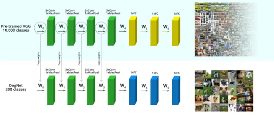
Finetuning, also called transfer learning, is a technique based on initializing the network’s weights with the weights of another already-trained network. Take for example the VGG network, which has been trained to recognize 1000 different types of objects. Its first 10 convolutional layers must have learned to recognize complex patterns for those objects. If we were to recognize another object, even if it is not among those 1000 classes, it makes sense to use those layers as our first layers too, because the network would already know what to look for. The alternative to finetuning is initializing the network either by random values or using probability distributions like the gaussian.

The main advantages of using finetuning over a plain random initialization are:

1. Better initialization yields more stable gradients, avoiding the common vanishing (tending to 0) and exploding (tending to∞) gradients problems

2. Faster learning, as the network already has good representations of the objects

Also, when transferring weights from one network to another, we may choose to: a)

freeze them and stop the network from modifying them at all,b)allow them to be modified but at a slower rate compared to other layers (by selectively decreasing its learning rate) or

c)treat them as another variable to be optimized.

The first approach is used when the trained network already has good representations for the problem we are facing. We consider its filters to be good enough to detect all kind of objects we might need. Likewise, the second case also assumes this, but allows small modifications for a better fitting on the current data.

Common sources of fine tuning are the VGG and the Alexnet [20] (or modifications of it), as its first convolutional layers are proven to have learned complex representations. Googlenet [25] and residual network are now being used too.

For example (Figure 11), the convolutional layers from the VGG network are used to initialize a new network which must predict dog breeds. Note that only the convolutional layers are taken, and its weights are frozen, but the remaining fully connected layers are trainable, so that it can adjust to the new categories to predict.

4.2.2 Residual Networks

Intuition might tell that deeper networks, consisting of more chained convolutional layers, might lead to more complex representations of the input data. This, although it is true, comes with hard to solve problems:

Figure 11: Finetuning of the VGG convolutional layers to classify doog breeds

1. Exploding or vanishing gradients: The gradient might tend to 0 (thus having no direction) or to explode and go out of the data range. This problem has been recently solved by the batch normalization layer, but classic strategies like better initialization or gradient clipping are still useful and help to prevent these issues.

2. Degrading gradient: A deeper network will see its gradient lose its reference to the input data, as in it will go so deep that the gradient will no longer hold meaningful information. This makes the accuracy to get saturated at a lower point than normal. Then, either it does not improve at all it worsens over time.

A recent paper from Microsoft defines an architecture they call Residual Networks which addresses and solves these problems. A normal neural network would stack its layers in a linear fashion (Figure 12a) while the Residual Networks take a different approach, they use residual blocks (Figure 12b).

(a) Traditional layer stacking (b) Residual block

Figure 12: Tradicional layer stacking approach vs residual blocks

A block is composed of two convolutional layers and two non-linearities (ReLU on the paper), with the particularity that before the last ReLU the input is summed to the acti-vations. This allows the network to propagate some remaining information of the original input (thus the name ofresidual networks).

It has been shown that using this strategy a network can go as deep as 1000 layers on the CIFAR-10 [26] dataset and of 152 layers (8 times the size of the VGG) on the imagenet dataset. Not only they successfully converge, but they also improve the previous best accuracy.

4.2.3 Color space

Although not strictly related to CNNs, choosing the right color space is fundamental for the network to work faster and better. The immediate and naive choice would be to use RGB color space, which consists of 3 channels that mix lighting (intensity) and colors all together. This, however, implies there is a high correlation between channels: increasing either one of them would increase the overall intensity of that pixel. While RGB is a good color space for humans to easily comprehend and visualize colors, it is not practical when it must be used for machine learning algorithms.

When looking for non-correlated color spaces, the most habitual are [27]:

1. YUV: It is usually employed for video or image processing, commonly seen in the PAL and NTSC specifications. It defines a luminance component (Y) and two chrominance channels (UV) where color is encoded.

2. HSV: From Hue/Saturation/Value, it may also be called HSI (intensity) or HCI (chroma or colorfulness) amongst others. The main advantage of this color space is being intuitive. Colors might increase intensity in a natural manner, increasing only Value, unlike RGB where you would have to increase each channel or YUV where you would likewise have to increase UV. It also features a separation (Value) of intensity from color.

3. L*a*b*: This color space is one of the created byComission Internationale de l´Éclairage

(CIE) and considered standard in many applications. All colors from CIE try to im-itate human vision and, as such, are based upon it. They achieve to be uncorrelated between lightness (L) and color (a,b) but fail to be easily interpretable.

Doing a brief recap we can easily see that the input image, a grayscale image, could be used as the luminance/intensity channel of either of these color spaces. Strictly checking the values one would see that the Y/V/L channels (respectively to each color space) are not exactly the same as the grayscale conversion of an RGB image, but the error is so low that any difference would not be noticeable. This means we could reduce the problem of outputting a 3 channels RGB image to a 2 channels YUV/HSV/L*a*b* image, as the remaining 3rd channel would already be the submitted image.

When choosing the final color space, HSV got discarded due to even being intuitive, it is not as powerful when it comes to encoding colors. Between YUV and CIE L*a*b*, the

decision was in favour of L*a*b* for a simple reason, it is more widely used and considered to be standard, while being backed by the CIE organization.

Tests were done to assure that using a color space with 2 channels for an image would be better than RGB, and all of them showed significant improvements. The final architecture was then completely based off the L*a*b* approach.

4.2.4 Final architecture

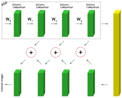
The final architecture is shown in Figure 13. It will be first globally described and then individually inspected.

Figure 13: Final fully convolutional architecture for image colorization. Each green block consists of one or more convolutions. The yellow block is a convolution of a 1x1 kernel. The summation is equivalent to the summation of the batch normalized green block above

and the convolved upsample of the activation of the green block below.

First of all, the image is forwarded through a subsection of the VGG network. Specifically, it includes all the first 4 blocks of convolutions, but where a block of three convolutions is used in the original VGG network, here a block of only two is used, due to memory constraints. All the weights of this section are fixed, so that they are not taken into account during the optimization process.

The VGG performs a Max Pooling after each convolution block, so, if we use an initial image of size 256x256, taking into account the convolutional layers have padding and we have a total of 4 poolings, the final size will be16x16. To restore the original size the network will also need to do 4 upsamplings.

Upsampling block: One important characteristic of the VGG network is that the number of parameters is constant all along the network. Whenever a pooling is done the resulting activations are reduced by half, but the number of filters on the next convolutions is doubled. The upsampling blocks, Figure 14, will follow the same logic, whenever the image (or activations) is doubled in size, the number of filters in the filters bank will be halved, thus achieving the constantness in parameters.

Figure 14: Closer look of the upsampling block

The upsampling might be done by using a bilinear filter, but for performance, a simpler nearest neighbor filter with 4-connectivity has been used. Both have been tested and no real impact is perceptible in the final image, neither color nor texture-wise.

Taking the same idea as the residual networks, the activation from the same level on the VGG is summed to the upsampled image, so that the gradient is more stable. To make it even more stable, before summing, the activation of the VGG network is forwarded through a batch normalization layer.

To allow the network to have more complex representations along with a bigger number of parameters, a convolution is also done to the upsampled image and to the summation

result. Otherwise, the network would have no parameters to optimize (as the VGG is fixed and neither the batch normalization nor the summations have any significant parameter).

The next block simply takes as input the result of the last convolved summation, and does the same operation but at a bigger size and with a lower number of filters.

Activations: The first tests were done using ReLUs as non-linearities after each con-volution. The network completely failed to color the image and would often output either grayscale images or sepia-colored images. Our color space, L*a*b*, uses numbers in the range[−128, 127], which we normalize to [−1, 1]. It is obvious then that if all our weights range from[0,∞), due to the ReLU, we can not represent the lower negative half.

That is why all the network now uses hyperbolic tangents as activation functions. Their derivatives are still easy and fast to compute and behave as expected, expanding the acti-vations to the whole range of the color space.

Network output: After the last upsampling block two more convolutions are per-formed, one with the same number of filters as the block and the last with only 2 filters. As we want to output a 2-channels image, this is exactly what the last layer does, converge to 2 outputs.

As a measure of error, or loss function, the mean of the euclidean distance between the target image and the resulting one is used:

E= 1

N(y−yˆ)

2

Where y is the target image and yˆ the resulting image. N depends on the batch size, the number of images fed at the same time to the network, but in general terms that is:

N=batch·256·256

5 Implementation

To implement the network two frameworks have been used, Caffe [28] and Tensorflow [29]. Both of them with its advantages and disadvantages. Many more libraries and frameworks exist, just to name a few: Theano, Neon and Microsoft CNTK.

5.1 Frameworks

5.1.1 Caffe

Its main backers are the Berkeley Vision Group. Caffe’s main feature is its performance and speed, being the fastest among all the frameworks at the time of writing this project. It is built in C++ and exposes a Python interface. All the networks must be written in ”Protocol Buffers” from Google4_{, which although makes the files clear and well structured,} it is not practical when one must write repeated structures. Its Python API allows defining custom layers but with a high performance cost. It is mostly focused on visualization and testing rather than network definitions.

Being the precursor of convolutional neural networks, it has a fine-tuned code and perfect integration with GPU acceleration through NVIDIA CUDA (and recently OpenCL). Part of its high performance comes from its hand-written derivatives. All layers must specify the derivatives and it does not include any automatic-differentiation system. It is also one of the best systems when it comes to memory usage, being able to fit large networks just fine.

5.1.2 Tensorflow

Recently open-sourced, it is the framework used internally by Google. Although it is not as fast as Caffe nor does manage memory as fine, it has a few advantages:

1. It includes auto differentiation, so when creating new operations or layers, there is no need to hand-write the derivatives, as they are automatically calculated

2. Fully exposed API to Python and many more languages, including network definition (graph) with built-in support for language specific constructions (such as for-loops, conditions...)

It features a complete set of functions for traditional neural networks, convolutional and recursive. Newer papers and techniques can easily be implemented thanks to its support for complex math operations and a supportive community.

More technical aspects of Tensorflow will be discussed below, referring specifically to the implemented architecture and better illustrating its functionality.

5.2

Network implementation

As Tensorflow came later, this project was started with Caffe. As soon as Tensorflow was available and stable enough, the whole architecture was ported to Tensorflow. Even though two different frameworks have been used, the core of the layers are exactly the same, so an initial general explanation will be done.

5.2.1 Optimizer

To optimize the network an Adam [30] optimizer has been used, tweaking the epsilon

parameter. It has been tested that problems like imagenet require an epsilon of_≈ [1, 0.1]. To find the appropriate learning rate and epsilon combination, a grid-search has been used. That is, all combinations of learning rate in[1·10−1, 1·10−4]and epsilons[1, 1·10−4]have been tested until the best one has been found. The net which converged faster and produced better results was using learning rate1·10−3_{and epsilon1·10}−3_{. To make it work better,}

a decaying exponential learning rate has also been used, every 1000 iterations the learning rate is exponentially decreased by0.95.

The batch size has also been tested to find the best one, compromising performance and results. A batch size of 1 image does≈5.25iterations per second, but fails to converge with good enough results. A batch size of 32 is slow, each iteration takes about 120 seconds, and the network takes too long to achieve good results. Any number higher does not fit in the memory of the GPU. Eventually, the batch size was set to 8, which yields goods results after a decent amount of time.

It has also been tested whether the network generalizes better by applying an L2 regu-larization to each weight (smoothing them) of either(0.001, 0.003, 0.05)or none at all. At the end, the version with no regularization worked better and produced better results.

5.2.2 Number of parameters

As said, the VGG network maintains the number of parameters constant (except the last that reduces dimensions for the next fully connected layers). Each one ordered as (width,height,channels)5:

256x256x64→ 128x128x128→ 64x64x256→ 32x32x512→ 16x16x512 ↓

256x256x64← 128x128x128← 64x64x256← 32x32x512← 16x16x1024

The second line corresponds to the upsampling blocks, after upsampling, convolving and summing. Finally, two more convolutions are performed to obtain the ab channels: →256x256x32→256x256x2.

We can calculate the number of parameters of a given convolutional layer by applying the formula: input_f ilters·kernel_height·kernel_width· f ilters+bias. The bias has size equal to f iltersin the equation above, as it is 1D. Knowing the upsample block consists of 2 convolutions, one with the same number of filters as the input and the other halved, we can easily calculate each of blocks parameters:

Initial =512·1·1·1024 =524288 U psample4 =(1024·3·3·512+512) + (512·3·3·256+256) =5899008 U psample3 =(256·3·3·256+256) + (256·3·3·128+128) =885120 U psample2 =(128·3·3·128+128) + (128·3·3·64+64) =221376 U psample1 =(64·3·3·64+64) + (64·3·3·32+32) =55392 FinalConv1 =32·3·3·32+32 =9248 Output =32·3·3·2+2 =578

We should also take into account that batch normalization layers have also 2 parameters. We have 4 layers of this type, which are 8 parameters in total. So, the network has

Total=524288+5899008+885120+221376+55392+9248+578+8=7595018

parameters to optimize.

5.2.3 Tensorflow specific

As the final architecture is done and presented in Tensorflow, a deeper explanation on how it works will be done in this section. Tensorflow has, as they say, a data oriented flow. When working with Tensorflow one has to think in terms of the graph, not as a functional programming language.

The graph is nothing but the assembled tree of all the operations, variables and place-holders defined. When you create either of these using the API it provides, no real calculus or operation is ever performed. It just stores the reference as a node in the graph and postpones the real operation.

To actually execute anything first a session must be started. Sessions are specific to devices, as operations, allowing to execute on GPU or CPU seamlessly. When the session is running, you can evaluate or run any expression on the graph. Such evaluation yields the real value. Doing so Tensorflow manages to:

1. Reduce all Python ↔C++ communication, which would slow down all processing 2. Keep an organized directed acyclic graph which can be navigated or executed

inde-pendently

When using this framework, the so far called weights or parameters are renamed to Variables. Any Tensorflow Variable will be a learnable parameter in the network, if not specified otherwise. Tensorflow allows to keep a hierarchical graph of variables by using

variable_scopes. They allow all variables inside the scope to be initialized in the same manner and keeps references to them grouped by the same common prefix, the scope’s name.

As Tensorflow operates separately, in the session, to pass variables from the Python/C side to the actual computational session, one must use placeholders. Unlike variables, place-holders are not trainable and its only purpose is for data loading.

It also comes with a wide range of functions to initialize weights and a huge variety of optimizers to train all the variables. Tensorflow does not, however, provide already done layers, as it only makes available mathematic operations. Supplied with this project code there are a few Python helper files which extend the framework:

1. Dataset.py: Usually datasets are big and do not fit in the main memory (RAM mem-ory). This file provides classes to procedurally load from the drives. Only a batch is loaded at once. Furthermore, the data is loaded asynchronously from a thread, using the Python Queue object which is thread-safe by default. The training and loading processes can be done at the same time, improving performance and reducing the amount of time it takes to train the network.

Supplied classes allow to load from a) text files, where each line is a combination of the image path and its class, b) LMDB files, using the Caffe format for image serialization and de-serialization and c) native numpy arrays, that although does not reduce memory usage it facilitates obtaining cyclic batches.

2. Models.py: It includes the definition of the VGG network graph, a reduced version of it, and some base classes to simplify models:

(a) LearningRateDecay: Tensorflow allows to have an exponential decay over the learning rate, but involves quite a few lines. This class simplifies it by grouping everything in a simple object, with no additional calls.

(b) Optimizer: Wraps the optimizer, allowing to easily clip gradients or apply de-caying learning rates. The methods exposed by this class are the same as the exposed by the original Tensorflow optimizers, to ease the usage.

(c) Model: When developing more than one model or architecture, many lines of code are the same. This class groups them and reduces the amount of code needed to get a functional model, letting the user concentrate in the important aspects. 3. Layers.py: Defines all layers as classes. They all inherit from a base class which defines

default values that can be tuned, for example, if variables are trainable or not. They are all based in the Tensorflow basic operations.

The main point on using classes is they make it easy to access the variables declared in the layer itself, as they are saved as attributes of the class itself.

4. Network.py: It basically defines all layers, but as bare functions instead of classes. They are more straightforward than the class based approach and might be faster to use if one simply wants to quickly define a model. It also implements methods to load saved numpy pre-trained models.

5.2.4 Visualization

An important part when doing neural networks is not only the results but the visualiza-tion of the network, which implies:

1. In our particular case, visualizing the results

2. Monitoring and validating the loss and accuracy (if it applies) of the network, to see possible under-fittings or over-fittings

3. Visualizing the learned filters on the convolutional layers, to see and verify they make sense

Here Jupyter notebooks (previously known as IPython notebooks) have been used. They are considered as the best option because they allow to interactively program and see the results inline. All of it within a browser and without needing physical access to the machine. Furthermore, it allows a wide range of languages to be used, like Python, Julia and R. Due to its fast programming and extensive libraries available, Python has been the language used. Caffe at some points had problems with Python and Julia was used as a backup.

To ease the process, OpenCV was used to do RGB _↔ L*a*b* conversions and image manipulations, such as resizing and reading from disk. Matplotlib served as the main plotting library, both for showing images and numeric results.

Tensorflow also comes with a visualization software called Tensorboard, which enables us to: a) see a complete graph of our network (Figure 15), b) see all tensors in the graph and c) inspect values all along the execution, including plots with average values, deviations... It has been widely used to see the real progress and its values will be further discussed.

5.3

Online website

Any user should be able to use this technique, but it is clear that the Python files provided require at least some basic programming knowledge. The programmed website allows inexperienced users to colorize images and at the same time serves to do quick tests. The website consists of three sections, one where the user is able to upload an image and the system will automatically colorize it; and two informative sections, the first which links to this document and the later which gives information about the author.

The user should also be able to supply images not in grayscale, thus the website must automatically convert them. Of course, if the input image already has color, it will be completely discarded and not used in the colorization process.

From the implemented website it will be analysed the backend (the server) and the frontend (the actual user-interactive side). The interaction will be explained in a different subsection, as it involves both sides. The whole implementation is supplied as source code and found in theWebServer folder.

It is completely integrated with the interface Tensorflow gives and runs fine using CPU only, so it could be deployed to a system which does not have GPUs.

The website, as seen in Figure 16, is available at: http://g-build-server.asuscomm. com:5000/

5.3.1 Backend

It is completely programmed using Python. The main reason behind using Python and not any other server-scripting language, like PHP, is that Tensorflow already exposes a complete API to Python, so no piping or communication with another Tensorflow process will be required.

Flask: It is one of the many webservers programmed for Python. Other alternatives, such as DJango and Bottle exist, but they come bloated with much more middleware and utilities which will never be used for this project (like an admin panel in case of DJango). Flask is lightweight and fast, and programming a website is easy and costless.

Creating a user visitable page with Flask is easy, it is defined as a Python function and decorated with a helper function from Flask. The decorator, usually@app.route(path), takes a parameter which corresponds to the URL for that page. Then, two options are available, either directly returning a string containing HTML code or parsing and rendering a template.

This project uses the templates engine provided by Flask, Jinja2. This engine allows to pass variables, even objects, arrays and dictionaries, from the Python side to the HTML template. Those variables get substituted and sent to the user as bare HTML. Templates allow to make a clear separation between the controller (Python) and the view (HTML), so they help to keep clean and understandable code.

This website is stateless, it maintains no information of the session, the user nor the uploaded images, so it does not require of sessions nor databases.

Gunicorn: Although Flask itself is capable of handling incoming connections and serv-ing requests, it is not powerful and saturates quite easily. Thankfully, we are not obligated to use it, we can use external webservers, like Gunicorn, nginx or Apache. Again, with the aim of keeping the code small, having as few dependencies as possible and being lightweight, Gunicorn has been chosen.

Gunicorn integrates perfectly with Flask and no adjustment has to be done in order for it to work. Even more important, our website is input/output (I/O) intensive, as it must read and convert an image, blocking meanwhile. A normal webserver, as Flask, would leave all connections hang until the conversion finished. Gunicorn, however, allows us to spawn more than 1 worker, so that when one is blocked the others can still work. This project uses 5 workers, although more could be used.

5.3.2 Frontend

The user receives a website done with HTML5, CSS3 and Javascript, based on a free available template called Grayscale6_{. Although it uses a template, none of the functionalities} here described were implemented beforehand, particularly the uploading process or the communication with the backend.

HTML5: Important features of the HTML5 language have been used for this website. To convert the input image to grayscale a <canvas> element is used combined with the Javascript object FileReader. Basically, the submitted image is read using the FileReader and drawn into the canvas, which allows to separately select each channel. It then averages the 3 RGB channels, obtaining a grayscale image. Drag and drop is also doable thanks to HTML5 and jQuery.

Javascript: It is used mainly through the jQuery library, which simplifies the syntax and provides useful functions for DOM manipulation. It is used to update the dragged images and the texts and elements that display the uploading and colorization progress.

It also simplifies all the AJAX communication, used to interchange messages with the backend without making the user reload the page or follow any link. This enables the user to do a transparent upload and colorization.

Also, jQuery introduces nice visual effects, like the upper menu and the smooth page scrolling when following links or visualizing the colorization result.

CSS3: It also uses an external library, called Bootstrap, to make the web fluid and adaptable to different screen sizes. It comes into special importance when visiting the website from a mobile device, because it is able to correctly rearrange to maintain a pleasant navigation.

Custom styles are used to make uploading process give feedback to the user. Also, achieved through CSS, the user can hover the mouse over the colorized image to see the original grayscale image.

5.3.3 Communication

As already advanced, AJAX is used to communicate the client with the server. The advantages of using AJAX are: a) being able to show a progress, both of the state, uploading or colorizing, and the percentage of the image uploaded and b) keep the user in the same page, without extended loading times.

Sending the image to the server is achieved through the Javascript object FormData, which enables to domultipart/form-datauploads. That means the body of a POST request might have different objects inside it, for example, files. The server then receives the image and colorizes it, converting to grayscale first if necessary. It also automates the L*a*b* conversion.

Sending back the colored image to the client is trickier. The easiest way would be to store the image in the server and then send a link to that image to the client, but that would mean occupying storage in the server, which is limited. HTML5 introduced a URL based method to display images, files and even music. An image can be encoded into an URL by first encoding it in base64, so that it is encoded with printable characters. Then, the URL is formed as: ”data:image/png;base64,” + ”encoded_base64_image”.

As this encoding works as a URL, it can be placed in the srcfield of an <img> node, making it display the image as if it was downloaded from a real URL. Changing this attribute can easily be done using jQuery, we send the encoded URL as the response to the AJAX request that uploads the image, thus making only a single connection in all the process.

6

Results

This section discusses the results obtained from the previously explained architectures and its later implementation. It introduces a standard way to quantitatively measure the quality and also discusses the images from a qualitative, human perceived, point of view. Examples of where the network gives good results and where it fails to produce the expected results will also be given and analysed.

6.1

Measure of quality

It has been said that to measure the error on the network and to make it learn, the euclidean distance between the target image and the obtained image has been used. This is a good function for a neural network as it is convex and can be easily derived, but it might not fit the way a human perceives the reality.

When working with images the quality measurement is usually done with Peak Signal-to-Noise Ratio (PSNR) [31]. This ratio is particularly used when using reconstructions of lossy codecs during image compression or decompression. It makes sense to think of this problem as a reconstruction problem (we are indeed recovering color), thus this measure is suitable. Its main advantage over a bare euclidean distance is that it approximates the human perception and its results are easier to interpret given the original and reconstructed images.

A higher PSNR value means the reconstruction is of better quality, being ∞ the best possible reconstruction and 0the worst. Figure 17 shows the different values of PSNR into context. The ratios of these images, however, have been obtained from a grayscale image and not an RGB, so they are merely for illustration purposes and should not be directly compared with the RGB use given from here on. PSNR might be calculated by:

PSNR=10·log10 ( MAX2 I MSE )

Where MAXI is the maximum pixel value for the image and MSEis the mean squared error: MSE= 1 256·256·3 3

∑

∑

∑

An important note, as seen in Equation 8, is that the comparison is done in the RGB color space. Although we could use the L*a*b* space, doing it in the RGB color space

comes into importance when comparing with other methods, for example state of the art implementations. Also, images should be in the range[0, 255], thus MAXI =255.

(a) PSNR = ∞, original (b) PSNR ≈ 30 (c) PSNR ≈ 25 (d) PSNR ≈ 20 (e) PSNR ≈ 15

Figure 17: PSNR values for Lena

Image by Rice University, Digital Image Processing ELEC 539

6.2 Datasets

To train and test the framework three completely different datasets have been used. The first one consists of synthetic images generated with the purpose of doing an initial test and verification of the problem. The other two, landscapes and faces, are used to prove the architecture is capable of obtaining good results whatever input is given. Of course, each dataset is trained separately and then tested with images of that same category.

Before showing the datasets results, a special mention must be done. The loss graphic obtained on each dataset will be shown, however, it may be misleading: there is a wide range of images on the datasets, for example, we might find landscapes with a blue sky or orange sunsets. If the network tries to minimize the first, the second would raise, and vice-versa. That is why even though during some iterations the loss might seem to be stuck, the resulting images have notable differences. The main interest on the loss is: a) to see if it seems to converge up to a point and b) to make sure the train and test loss are about the same, so that no overfitting is happening.

6.2.1 Synthetic data

The original problem relies on coloring images of size 256x256, which is more than the usual 28x28 or 80x80 most neural networks use. Approaching the problem by trying to colorize the full 256x256 resolution landscape images would have been a bad idea because:

1. It was uncertain if the problem, colorizing an image, would be able to be solved 2. The time spent to pre-process the original images would have been much greater than