Exploring Temporal Information for Improved Video Understanding

(1)

UC Merced Electronic Theses and Dissertations

Title

Permalink

https://escholarship.org/uc/item/1mj9c846

Author

Zhu, Yi

Publication Date

2019 Peer reviewed|Thesis/dissertation

eScholarship.org Powered by the California Digital Library University of California

(2)

UNIVERSITY OF CALIFORNIA, MERCED

A dissertation submitted in partial satisfaction of the requirements for the degree of

Doctor of Philosophy in

Electrical Engineering & Computer Science by

Yi Zhu

Committee in charge:

Professor Shawn Newsam, Chair Professor Trevor Darrell

Professor Ming-Hsuan Yang

(3)

(4)

The dissertation of Yi Zhu is approved, and it is acceptable in quality and form for publication on microfilm and electronically:

Professor Trevor Darrell

Professor Ming-Hsuan Yang

Professor Shawn Newsam, Chair

University of California, Merced

2019

(5)

(6)

TABLE OF CONTENTS

Signature Page . . . iii

Table of Contents . . . v

List of Figures . . . ix

List of Tables . . . xiii

Acknowledgements . . . xv

Vita and Publications . . . xvi

Abstract . . . xviii

Chapter 1 Introduction . . . 1

1.1 Human Action Recognition . . . 1

1.2 Semantic Segmentation for Autonomous Driving . . . 4

1.3 Dissertation Overview . . . 5

Chapter 2 Embedded Depth for Action Recognition . . . 8

2.1 Introduction . . . 8

2.2 Related Work . . . 10

2.3 Methodology . . . 12

2.3.1 Depth Extraction . . . 12

2.3.2 Spatio-Temporal Depth Normalization . . . 13

2.3.3 CNNs Architecture Selection . . . 14

2.3.4 Depth-Temporal Stream . . . 14

2.3.5 CNNs: Feature Extraction or End-to-End Classification . 15 2.4 Experiments . . . 16

2.4.1 Datasets . . . 17

2.4.2 Implementation Details . . . 17

2.4.3 Results . . . 18

2.4.4 Discussion . . . 20

2.4.5 Comparison with State-of-the-art . . . 21

2.5 Conclusion . . . 22

Chapter 3 Hidden Two-Stream Networks . . . 23

3.3 Hidden Two-Stream Networks . . . 28

3.3.1 Unsupervised Optical Flow Learning . . . 28

3.3.2 Projecting Motion Features to Actions . . . 33

3.3.3 Hidden Two-Stream Networks . . . 35

3.4 Experiments . . . 35

3.4.1 Datasets . . . 35

(7)

3.4.4 Comparison to RNN and 3D CNN Approaches . . . 39

3.5 Discussion . . . 40

3.5.1 Ablation Studies for MotionNet . . . 40

3.5.2 CNN Architecture Search . . . 42

3.5.3 Stacking or Branching . . . 43

3.5.4 Learned Optical Flow . . . 44

3.6 Comparison to State-of-the-Art real-time approaches . . . 47

Chapter 4 Learning Optical Flow . . . 49

4.2 Guided Optical Flow Learning . . . 49

4.2.1 Proxy Ground Truth Guidance . . . 50

4.2.2 Unsupervised Fine Tuning . . . 52

4.2.3 Datasets . . . 53

4.2.4 Implementation . . . 54

4.2.5 Results and Discussion . . . 54

4.2.6 Comparison to State-of-the-Art . . . 56

4.2.7 Conclusion . . . 56

4.3 DenseNet for Dense Flow . . . 57

4.3.1 DenseNet Review . . . 59

4.3.2 Fully Convolutional DenseNet . . . 59

4.3.3 Unsupervised Motion Estimation . . . 60

4.3.4 Implementation . . . 61

4.3.5 Results and Discussion . . . 62

4.3.6 Comparison to State-of-the-Art . . . 62

4.4 Learning Optical Flow via Dilated Networks and Occlusion Rea-soning . . . 64

4.4.1 Dilated Networks . . . 65

4.4.2 Degridding . . . 67

4.4.3 Unsupervised Motion Estimation . . . 67

4.4.4 Occlusion Reasoning . . . 68

4.4.5 Datasets . . . 69

4.4.6 Results . . . 69

4.4.7 Generalization . . . 70

4.5 Learning Optical Flow Conclusion . . . 71

Chapter 5 Random Temporal Skipping for Multirate Video Analysis . . . 73

5.3 Approach . . . 76

5.3.1 Random Temporal Skipping . . . 76

5.3.2 Two-Stream Network Details . . . 77

(8)

5.3.3 Compact Bilinear Encoding . . . 80 5.3.4 Spatio-Temporal Fusion . . . 80 5.4 Experiments . . . 81 5.4.1 Trimmed Video . . . 81 5.4.2 Untrimmed Video . . . 85 5.4.3 Comparison to State-of-the-Art . . . 87 5.5 Conclusion . . . 88

Chapter 6 Universal Representation for Unseen Action Recognition . . . 89

6.3 Approach . . . 93

6.3.1 Generalized Multiple-Instance Learning . . . 93

6.3.2 Universal Representation Learning . . . 94

6.3.3 Computational Complexity Analysis . . . 98

6.3.4 Semantic Adaptation . . . 99

6.4.1 Settings . . . 99

6.4.2 Comparison with State-of-the-art Methods . . . 101

6.4.3 In-depth Analysis . . . 103

Chapter 7 Improving Semantic Segmentation via Video Propagation and Label Relaxation . . . 105

7.3 Methodology . . . 109

7.3.1 Video Prediction . . . 109

7.3.2 Joint Image-Label Propagation . . . 110

7.3.3 Improved Label Prediction . . . 112

7.3.4 Boundary Label Relaxation . . . 112

7.4.1 Implementation Details . . . 113

7.4.2 Cityscapes . . . 115

7.4.3 CamVid . . . 120

7.4.4 KITTI . . . 121

7.5 Implementation Details and Additional Result . . . 122

7.5.1 More Details of Our Video Prediction Models . . . 122

7.5.2 Non-Accumulated and Accumulated Comparison . . . 123

7.5.3 More Training Details on Cityscapes . . . 124

7.5.4 Failure Cases on Cityscapes . . . 124

7.5.5 Class Breakdown on CamVid . . . 125

Chapter 8 Conclusion and Future Work . . . 127

8.2 Future Work . . . 128

(9)

(10)

LIST OF FIGURES

Figure 1.1: Example scenarios where human action recognition can play a role. . . 2 Figure 1.2: Visual examples of semantic segmentation (classes are color encoded). 4 Figure 1.3: An overview diagram of my dissertation. . . 6 Figure 2.1: Action classes comparison: (a) “CricketBowling” and (b) “CricketShot”.

Depth information about the bowler and the batters is key to telling these two classes apart. Our proposed depth2action approach exploits the depth information that is embedded in the videos to perform large-scale action recognition. . . 9 Figure 2.2: Depth2Action framework. Top: Our depth two-stream model. Depth

maps are estimated on a per-frame basis and input to a depth-spatial net. Modified depth motion maps (MDMMs) are derived from the depth maps and input to a depth-temporal net. Features are extracted, concatenated and input to two support vector machine (SVM) classifiers, to obtain the final prediction scores. Bottom: Ourdepth-C3D framework which is similar except the depth maps are input to a single depth-C3D net which jointly captures spatial and temporal depth information. . . 10 Figure 2.3: Depth maps estimated from the video v ThrowDiscus g05 c02.avi in the

UCF101 dataset. (a): raw RGB frames; (b): depth maps extracted using [98]; (c): depth maps extracted using [41]; (d): the absolute difference between consecutive depth maps in (c). Blue indicates smaller values and yellow larger ones. . . 12 Figure 2.4: (a) Recognition results on the first split of UCF101. Plot showing the

classes for which our proposed depth2action framework (yellow) out-performs RGB-spatial (blue) and RGB-temporal (green) streams. (b) Visualizing the convolutional feature maps of four models: RGB-spatial, RGB-temporal, depth-spatial, and depth-temporal. Pairs of inputs and resulting feature maps are shown for each model for two actions, “Criket-Bowling” and “ThrowDiscus”. . . 19 Figure 2.5: Sample video frames of action classes that benefit from depth

informa-tion. Left: UCF101. Right: HMDB51. . . 20 Figure 3.1: Illustration of proposed hidden two-stream networks. MotionNet takes

consecutive video frames as input and estimates motion. Then the tem-poral stream CNN learns to project the motion information to action labels. Late fusion is performed to combine spatio-temporal informa-tion. Both streams are end-to-end trainable. . . 24 Figure 3.2: Branched temporal stream CNN. The convolutional features are shared

between optical flow estimation and action classification tasks. . . 35 Figure 3.3: Visual comparisons of estimated flow field from TV-L1, MotionNet

and FlowNet2. Left: ApplyEyeMakeup, BabyCrawling, BodyWeight-Squats, BoxingPunchingBag and CleanAndJerk. Right: Hammering, PlayingFlute, PommelHorse, WallPushups and YoYo. This figure is best viewed in color. . . 45

(11)

truth flow. ./ represents the inverse warping and unsupervised recon-struction loss with respect to the input image pairs. . . 51 Figure 4.2: Visual examples of predicted optical flow from different methods. Top

two are from Sintel, and bottom two from KITTI. . . 55 Figure 4.3: An overview of our unsupervised learning framework based on dense

blocks (DB). “Down” is the transition down layer, and “Up” is the tran-sition up layer. The orange colored arrows indicate the skip connections. See more details in Section 4.3.2. . . 58 Figure 4.4: Visual examples of predicted optical flow from different methods. Top

two are from Sintel, and bottom two from KITTI. . . 60 Figure 4.5: Upper: original FlowNetS. Bottom: our unsupervised learning

frame-work based on dilated convolution. For the three dilated convolutions (green), d2 and d4 denote a dilation factor of 2 and 4, respectively. The figure is best viewed in color. . . 66 Figure 4.6: Our bidirectional framework, whose weights are shared for both forward

and backward flow estimation. . . 69 Figure 5.1: Sample video frames of three actions: (a) playingguitar (b) wallpushup

and (c) diving. (a) No temporal analysis is needed because context in-formation dominates. (b) Temporal analysis would be helpful due to the regular movement pattern. (c) Only the last four frames have fast motion, so multirate temporal analysis is needed. . . 75 Figure 5.2: Overview of our proposed framework. Our contributions are three

fold: (a) random temporal skipping for temporal data augmentation; (b) occlusion-aware MotionNet for better motion representation learn-ing; (c) compact bilinear encoding for longer temporal context. . . 78 Figure 5.3: Top-10 classes that benefit most (top) and least (bottom) in UCF101 . 83

Figure 5.4: Sample visualizations of UCF101 dataset to show the impact of rea-soning occlusion during optical flow estimation. Left: overlapped image pairs. Middle: MotionNet without occlusion reasoning. Right: Motion-Net with occlusion reasoning. The figure is best viewed in color. We can observe the clear improvement brought by occlusion reasoning. . . 85 Figure 5.5: Action recognition accuracy on ActivityNet. We observe that the longer

temporal context we utilize, the better performance we obtain. . . 86 Figure 6.1: The proposed CD-UAR pipeline: 1) Extract deep features for each frame

and summarize the video by essential components that are kernelized by GMIL; 2) Preserve shared components with the label embedding to achieve UR using NMF with JSD; 3) New concepts can be represented by UR and adjusted by domain adaptation. Test (green line): unseen actions are encoded by GMIL using the same essential components in ActivityNet to achieve a matching using UR. . . 90 Figure 6.2: Visualization of feature distributions of action ‘long-jump’ and

‘triple-jump’ in the ActivityNet dataset using tSNE. . . 94

(12)

Figure 6.3: Convergence analysis with respect to# iterations. (1) is the overall loss in Eq. 6.2. (2) is the JSD loss. (3) and (4) show decomposition losses of A and B, respectively. . . 102 Figure 7.1: Framework overview. We propose joint image-label propagation to scale

up training sets for robust semantic segmentation. The green dashed box includes manually labelled samples, and the red dashed box includes our propagated samples. T is the transformation function learned by the video prediction models to perform propagation. We also propose boundary label relaxation to mitigate label noise during training. Our framework can be used with most semantic segmentation and video pre-diction models. . . 106 Figure 7.2: Motivation of joint image-label propagation. Row 1: original frames.

Row 2: propagated labels. Row 3: propagated frames. The red and green boxes are two zoomed-in regions which demonstrate the mis-alignment problem. Note how the propagated frames align perfectly with propa-gated labels as compared to the original frames. The black areas in the labels represent a void class. (Image brightness has been adjusted for better visualization.) . . . 109 Figure 7.3: Motivation of boundary label relaxation. For the entropy image, the

lighter pixel value, the larger the entropy. We find that object bound-aries often have large entropy, due to ambiguous annotations or propa-gation distortions. The green boxes are zoomed-in figures showing such distortions. . . 111 Figure 7.4: Boundary label relaxation leads to higher mIoU at all propagation

lengths. The longer propagation, the bigger the gap between the solid (with label relaxation) and dashed (without relaxation) lines. The black dashed line represents our baseline (79.46%). x-axis equal to 0 indicates no augmented samples are used. For each experiment, we perform three runs and report the mean and sample standard deviation as the error bar [19]. . . 116 Figure 7.5: Our learned motion vectors from improved label prediction are better

than optical flow (FlowNet2). Left (Qualitative result): The learned motion vectors are better in terms of occlusion handling. Right (Quanti-tative result): The learned motion vectors are better at all propagation lengths in terms of mIoU. . . 117 Figure 7.6: Visual comparisons on Cityscapes. The images are cropped for better

visualization. We demonstrate our proposed techniques lead to more accurate segmentation than our baseline. Especially for thin and rare classes, like street light and bicycle (row 1), signs (row 2), person and poles (row 3). Our observation corresponds well to the class mIoU im-provements in Table 7.3. . . 119

(13)

situations with multiple cars (row 1), dense crowds (row 2) and thin ob-jects (row 3). The bottom two rows show failure cases. We mis-classify a reflection in the mirror (row 4) and a model inside the building (row 5) as person (red boxes). . . 120 Figure 7.8: Visual comparison between our results and those of the winning entry

[23] of ROB challenge 2018 on KITTI. From left to right: image, pre-diction from [23] and ours. Boxes indicate regions in which we perform better than [23]. Our model can predict semantic objects as a whole (bus), detect thin objects (poles and person) and distinguish confusing classes (sidewalk and road, building and sky). . . 121 Figure 7.9: Failure cases (in yellow boxes). From left to right: image, ground truth,

prediction and their difference. Green boxes are zoomed in regions for better visualization. Rows (a) to (d) show class confusion problems. Our model has difficulty in segmenting: (a) car and truck, (b) person and rider, (c) wall and fence, (d) terrain and vegetation. Rows (e) and (f) show challenging cases when the object is far away, strongly occluded, or overlaps other objects. The last two rows show two training samples with wrong annotations: (h) mislabeled motorcycle to bicycle and (i) mislabeled fence to building. . . 126

(14)

LIST OF TABLES

Table 2.1: Recognition performance of our proposed configurations on three bench-mark datasets. (a): Our spatio-temporal depth normalization (STDN) indicated by (N) is shown to improve performance for all configurations on all datasets. (b): Using the CNNs to extract features is better than using them as end-to-end classifiers. Also, early fusion of features is bet-ter than late fusion of SVM probabilities. See the text for discussion on

depth two-stream versus depth-C3D . . . 16

Table 2.2: Comparison with the state-of-the-art. ∗ indicates the results are from our implementation of the method. Two-stream and C3D here is RGB based 22 Table 3.1: Our stacked temporal stream. Top: MotionNet. Bottom: traditional tem-poral stream. M is the number of action categories. Str: stride. Ch I/O: number of channels of input/output features. In/Out Res: input/output resolution. . . 29

Table 3.2: Architecture of Tiny-MotionNet. . . 32

Table 3.3: Comparison of accuracy and efficiency. Top section: Two-stage temporal stream approaches. Middle Section: End-to-end temporal stream ap-proaches. Bottom Section: Two-stream apap-proaches. . . 37

Table 3.4: Comparison to RNN and 3D CNNs based approaches. . . 39

Table 3.5: Ablation study of good practices employed in MotionNet. . . 41

Table 3.6: CNN architecture search. . . 42

Table 3.7: Stacking VS. Branching. . . 43

Table 3.8: Evaluation of optical flow and action classification. For flow evaluation, lower error is better. For action recognition, higher accuracy is better. . 44

Table 3.9: Comparison to state-of-the-art real-time approaches on four benchmarks with respect to mean classification accuracy. . . 46

Table 4.1: Results reported using average EPE, lower is better. Bottom section shows our guided learning results, the models are trained using the Flow-Fields proxy ground truth. The last row includes fine tuning. . . 53

Table 4.2: State-of-the-art comparison, runtime is reported in seconds per frame. Top: Classical approaches. Middle: CNN-based approaches. Bottom: Ours. ∗ indicates the algorithm is evaluated using CPU, while the rest are on GPU. . . 57

Table 4.3: Optical flow estimation results on the test set of Chairs, Sintel and KITTI. All performances are reported using average EPE, lower is better. Top: Comparison of different architectures with classical upsampling. Bottom: Our proposed DenseNet with dense block upsampling. . . 61

Table 4.4: State-of-the-art comparison. Runtime is reported in seconds per frame. Top: Classical approaches. Bottom: CNN-based approaches. ∗ _indicates the algorithm is evaluated using CPU, while the rest are on GPU. . . . 63

Table 4.5: Accuracy comparison of recent unsupervised approaches on KITTI 2012 and 2015 optical flow benchmarks. F1-all is measured in %. . . 70

(15)

Table 5.1: Necessity of multirate analysis. RTS indicates random temporal skip-ping. Fixed sampling means we sample the video frames by a fixed length (numbers in the brackets, e.g., 1, 3, 5 frames apart). Random sampling indicates we sample the video frames by a random length of frames apart. 82 Table 5.2: Comparison with various feature aggregation methods on UCF101 and

HMDB51. Compact bilinear pooling achieves the best performance in terms of classification accuracy. . . 83 Table 5.3: Comparison to state-of-the-art approaches in accuracy (%). . . 87 Table 6.1: Comparison with state-of-the-art methods using standard low-level

fea-tures. Last two sets of results are just for reference. T: transductive; I: inductive; Results are in %. . . 100 Table 6.2: Comparison with state-of-art methods on different splits using deep features.101 Table 6.3: In-depth analysis with baseline approaches. ‘Ours’ refers to the complete

pipeline with deep features, GMIL kernel embedding, URL with NMF and JSD, and TJM. (Results are in %). . . 102 Table 7.1: Effectiveness of Mapillary pre-training and class uniform sampling on both

fine and coarse annotations. . . 112 Table 7.2: Comparison between (1) label propagation (LP) and joint propagation

(JP); (2) video prediction (VPred) and improved label prediction (VRec). Using the proposed improved label prediction and joint propagation tech-niques, we improve over the baseline by 1.08% mIoU (79.46%80.54%). 114 Table 7.3: Per-class mIoU results on Cityscapes. Top: our ablation improvements

on the validation set. Bottom: comparison with top-performing models on the test set. . . 117 Table 7.4: Results on the CamVid test set. Pre-train indicates the source dataset on

which the model is trained. . . 122 Table 7.5: Results on KITTI test set. . . 123 Table 7.6: Accumulated and non-accumulated comparison. The numbers in brackets

are the sample standard deviations. . . 124 Table 7.7: Per-class mIoU results on CamVid. Comparison with recent top-performing

models on the test set. ‘SS’ indicates single-scale inference, ‘MS’ indicates multi-sclae inference. Our model achieves the highest mIoU on 8 out of 11 classes (all classes but tree, sky and sidewalk). This is expected because our synthesized training samples help more on classes with small/thin structures. . . 125

(16)

ACKNOWLEDGEMENTS

First, I would like to express my deepest gratitude to my PhD advisor, Professor Shawn Newsam, for supporting me over the years. He encouraged me to explore new directions and mentored me on how to be a good researcher. Most importantly, he taught me how to be a better person with integrity and humility.

I am also grateful to my committee, Professor Trevor Darrell and Professor Ming-Hsuan Yang for the time and effort they spent to help me prepare my dissertation and serve as my committee members.

I would like to thank my friends and co-authors, Xueqing Deng, Alex Hauptmann, Zhenzhong Lan, Yang Long, Ling Shao, Jia Xue and many others. It was fantastic to have the opportunity to work with these guys.

I appreciate my internship days at HikVision Research and Nvidia Research. My thanks go to Bryan Catanzaro, Zhe Hu, Matthieu Le, Edward Liu, Guilin Liu, Sifei Liu, Fitsum Reda, Karan Sapra, Kevin Shih, Deqing Sun and Andrew Tao for much help along the way. I could never have imagined more enjoyable internship experiences.

Last but not least, I am deeply indebted to the love and support from my wife Yani Zhang. This dissertation would not have been possible without her.

(17)

2011 B. S. in Electrical Engineering, Northwestern Polytechnical University, Xian. Advisor: Jianfeng Chen

2014 M. S. in Electrical Engineering, University of Kansas, Lawrence. Advisor: Lingjia Liu

2019 Ph. D. in Computer Science, University of California, Merced,

Merced. Advisor: Shawn Newsam

PUBLICATIONS

Yi Zhu, Karan Sapra, Fitsum A. Reda, Kevin J. Shih, Shawn Newsam, Andrew Tao and Bryan Catanzaro, Improving Semantic Segmentation via Video Propagation and Label Re-laxation, IEEE Conference on Computer Vision and Pattern Recognition (CVPR), 2019 (Oral)

Yi Zhu, Xueqing Deng and Shawn Newsam, Fine-Grained Land Use Classification at the City Scale Using Ground-Level Images, IEEE Transactions on Multimedia, 2019

Yi Zhu, Zhenzhong Lan, Shawn Newsam and Alexander G. Hauptmann, Hidden Two-Stream Convolutional Networks for Action Recognition, Asian Conference on Computer Vision (ACCV), 2018

Yi Zhu, Jia Xue and Shawn Newsam, Gated Transfer Network for Transfer Learning,Asian Conference on Computer Vision (ACCV), 2018

Yi Zhu and Shawn Newsam, Random Temporal Skipping for Multirate Video Analysis, Asian Conference on Computer Vision (ACCV), 2018

Xueqing Deng, Yi Zhu and Shawn Newsam, What Is It Like Down There? Generating Dense Ground-Level Views and Image Features From Overhead Imagery Using Conditional Gen-erative Adversarial Networks, ACM International Conference on Advances in Geographic Information Systems (SIGSPATIAL), 2018 (Oral)

Yi Zhu and Shawn Newsam, Learning Optical Flow via Dilated Networks and Occlusion Reasoning,IEEE International Conference on Image Processing (ICIP), 2018

Xueqing Deng, Yi Zhu and Shawn Newsam, Spatial Morphing Kernel Regression For Fea-ture Interpolation, IEEE International Conference on Image Processing (ICIP), 2018

Yi Zhu, Yang Long, Yu Guan, Shawn Newsam and Ling Shao, Towards Universal Represen-tation for Unseen Action Recognition, IEEE Conference on Computer Vision and Pattern Recognition (CVPR), 2018

Yi Zhu, Sen Liu and Shawn Newsam, Large-Scale Mapping of Human Activity using Geo-Tagged Videos, ACM International Conference on Advances in Geographic Information Systems (SIGSPATIAL), 2017

(18)

Yi Zhu and Shawn Newsam, DenseNet for Dense Flow,IEEE International Conference on Image Processing (ICIP), 2017 (Oral)

Yi Zhu, Zhenzhong Lan, Shawn Newsam and Alexander G. Hauptmann, Guided Optical Flow Learning, IEEE Conference on Computer Vision and Pattern Recognition (CVPR) Workshop, 2017

Zhenzhong Lan, Yi Zhu, Alexander G. Hauptmann and Shawn Newsam, Deep Local Video Feature for Action Recognition,IEEE Conference on Computer Vision and Pattern Recog-nition (CVPR) Workshop, 2017 (Oral)

Yi Zhu and Shawn Newsam, Efficient Action Detection in Untrimmed Videos via Multi-Task Learning, IEEE Winter Conference on Applications of Computer Vision (WACV), 2017 (Oral)

Yi Zhu and Shawn Newsam, Spatio-Temporal Sentiment Hotspot Detection using Geo-tagged Photos, ACM International Conference on Advances in Geographic Information Systems (SIGSPATIAL), 2016

Yi Zhu and Shawn Newsam, Depth2Action: Exploring Embedded Depth for Large-Scale Action Recognition, European Conference on Computer Vision (ECCV) Workshop, 2016 (Oral)

Yi Zhu and Shawn Newsam, Land Use Classification using Convolutional Neural Networks Applied to Ground-Level Images, ACM International Conference on Advances in Geo-graphic Information Systems (SIGSPATIAL), 2015 (Best Poster Award)

(19)

by Yi Zhu

In this dissertation, I present my work towards exploring temporal information for better video understanding. Specifically, I have worked on two problems: action recognition and semantic segmentation. For action recognition, I have proposed a framework, termed hidden two-stream networks, to learn an optimal motion representation that does not require the computation of optical flow [209]. My framework alleviates several challenges faced in video classification, such as learning motion representations, real-time inference, multi-framerate handling, generalizability to unseen actions, etc. For semantic segmentation, I have introduced a general framework that uses video prediction models to synthesize new training samples [217]. By scaling up the training dataset, my trained models are more accurate and robust than previous models even without modifications to the network architectures or objective functions.

Along these lines of research, I have worked on several related problems. I performed the first investigation into depth for large-scale video action recognition where the depth cues are estimated from the videos themselves [211]. I further improved my hidden two-stream networks [209] for action recognition through several strategies, including a novel random temporal skipping data sampling method [215], an occlusion-aware motion estima-tion network [214] and a global segment framework [92]. For zero-shot acestima-tion recogniestima-tion, I proposed a pipeline using a large-scale training source to achieve a universal representation that can generalize to more realistic cross-dataset unseen action recognition scenarios [210]. To learn better motion information in a video, I introduced several techniques to improve optical flow estimation, including guided learning [208], DenseNet upsampling [212] and occlusion-aware estimation [214].

I believe videos have much more potential to be mined, and temporal information is one of the most important cues for machines to perceive the visual world better.

(20)

Chapter 1 Introduction

The medium of information has expanded from texts, to images, and now to videos. Video data plays an important role in our daily life. YouTube recently reported that it now has more than 1.5 billion monthly active users, second only to Facebook, and viewers spend more time on YouTube than Facebook [1]. There are also millions of video cameras (such as surveillance cameras and in-vehicle cameras) in operation around the world that need to be analyzed for security concerns. With 300 hours of video being uploaded to YouTube and petabytes of data generated by the video cameras every minute, it is not possible to understand this large corpus of video data through human effort. Only machine vision can accomplish this.

Automatically localizing, detecting and recognizing objects and humans in long uncon-strained videos can save tremendous time and effort for a variety of applications, including video recommendation, scene understanding, video summarization, surveillance monitoring, etc. In this dissertation, I focus on two specific problems in video understanding: (i) auto-matic recognition of human actions and (ii) semantic segmentation in autonomous driving scenarios.

1.1 Human Action Recognition

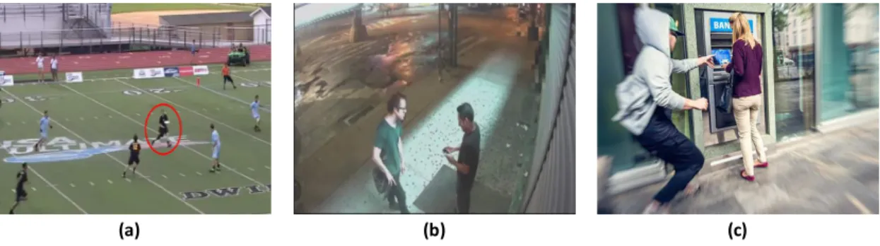
Human action recognition is a task that requires understanding of what activity the human is doing in a video. Figure 1.1 shows some specific examples where human action recognition can play a role. Video retrieval would be more accurate if we can do content-based action recognition so that we know Figure 1.1 (a) is about a group of people actually playing frisbee on a football field. Surveillance video cameras would be more intelligent if

(21)

(a) (b) (c)

Figure 1.1: Example scenarios where human action recognition can play a role.

they can monitor and forecast people’s activities, e.g., people are just talking or preparing to fight each other in Figure 1.1 (b). The police would catch the thief more quickly if the smart phone cameras can detect the robbery in Figure 1.1 (c) and automatically send out alarms.

However, despite the increasing importance of video action recognition, the ability to analyze it in an automated fashion is still limited. Human action recognition is particu-larly hard due to the enormous variation in the visual appearance of people and actions, camera viewpoint changes, ill-defined categorization, moving background, occlusions, and the large amount of video data. The current state-of-the-art approach is a two-stream convolutional network [144] in which spatial stream models appearance using the video frames, and a temporal stream models motion using pre-computed optical flow. Despite its superior performance, the two-stream network [144] and its extensions [164, 165, 37, 27] still face challenges, including real-time inference, long temporal reasoning, multi framerate handling, online action detection, generalizability to unseen actions, etc. Specifically, there are several questions that need to be answered.

• First, do we need optical flow? Can other representations help us differentiate actions better?

• Second, is optical flow the best motion representation? Can we learn optimal motion representation in CNNs for real-time action recognition?

• Third, can we learn a universal representation that can generalize to unseen actions without model re-training?

In the first half of my dissertation, I address the questions mentioned above. I briefly describe the motivation, the methodology and the results of my past work below.

(22)

3

Starting with the seminal two-stream CNN method [144], approaches have been limited to exploiting static visual information through frame-wise analysis and/or translational mo-tion through optical flow. Further increase in performance on benchmark datasets has been mostly due to the higher capacity of deeper networks and better training regularization. In my ECCV 2016 workshop paper [211], I raise the question of whether other representations like depth or human pose can help classify actions? I perform the first investigation into depth for large-scale video action recognition where the depth cues are estimated from the videos themselves. I demonstrate that using depth is complementary to existing approaches which exploit spatial and translational motion information and, when combined with them, achieves state-of-the-art performance. However, depth estimation from videos was not very accurate at that time, and so the improvement was only marginal. I thus turned back to two-stream methods that use video frames and optical flow.

As for two-stream approaches, there are two main drawbacks: (i) The pre-computation of optical flow is time consuming and storage demanding compared to the CNN step. Even when using GPUs, optical flow calculation has been the major computational bottleneck of the current two-stream approaches; (ii) Traditional optical flow estimation is completely independent of the high-level final tasks like action recognition and is therefore potentially sub-optimal. It is not end-to-end trainable, and therefore we cannot extract motion infor-mation that is optimal for the desired task. In my ACCV 2018 paper [209], I raise the question of whether we can learn a better motion representation than optical flow in an end-to-end network and avoid the high computational cost at the same time? I present a novel CNN architecture that implicitly captures motion information between adjacent frames. My proposed hidden two-stream CNNs take raw video frames as input and directly predict action classes without explicitly computing optical flow. My end-to-end approach is 10x faster at inference than a two-stage one. Experimental results on four challenging action recognition datasets, UCF101, HMDB51, THUMOS14 and ActivityNet v1.2, show that my approach significantly outperforms the previous best real-time approaches.

I further improve my hidden two-stream networks [209] by several strategies, including a novel data sampling method, an occlusion-aware motion estimation network [214] and a global segment framework [92]. In my ACCV 2018 paper [215], I propose a random temporal skipping technique that can simulate various motion speeds for better action modeling and make the training more robust. My framework achieves state-of-the-art results on six large-scale video benchmarks, demonstrating its effectiveness for both short trimmed videos and long untrimmed videos.

(23)

Figure 1.2: Visual examples of semantic segmentation (classes are color encoded).

Although I am able to achieve promising results on action recognition benchmarks, e.g. 98.0% on UCF101, generalizing the models to recognizing unseen actions remains a challenge. The excellent performance on the benchmarks is due to the large amounts of annotated data, thanks to recently released large-scale video datasets. However, for real world applications, such as anomaly detection in surveillance videos, there typically is not sufficient training data to train a decent model. In my CVPR 2018 paper [210], I propose a pipeline using a large-scale training source to achieve a universal representation that can generalize to a more realistic cross-dataset unseen action recognition scenarios. I first address the task as a generalized multiple-instance learning problem and discover building-blocks from the large-scale ActivityNet dataset [59] using distribution kernels. Then I propose the universal representation learning (URL) algorithm, which unifies non-negative matrix factorization with a Jensen-Shannon divergence constraint. The resultant universal representation can substantially preserve both the shared and generative bases of visual semantic features. A new action can be directly recognized using such a representation during tests without further training. Extensive experiments demonstrate that my URL algorithm outperforms state-of-the-art approaches in inductive zero shot action recognition scenarios using either low-level or deep features.

1.2 Semantic Segmentation for Autonomous Driving

Semantic segmentation is a long standing computer vision task which requires predict-ing dense semantic labels for every image pixel. Some examples can be seen in Figure 1.2 where different classes are segmented and encoded in different colors, such as person (red), car (blue), vegetation (green), etc. Due to the excessive need of autonomous driving, seman-tic segmentation has advanced rapidly in the last five years [8, 202, 178, 23, 32]. However, most approaches still focus on image segmentation because of insufficient labeled data and expensive computation.

(24)

5

In reality, most semantic segmentation datasets have the video recordings such as in autonomous driving scenario, but they are sparsely annotated at regular intervals. For example, Cityscapes [34] is one of the largest and most popular semantic segmentation datasets. The video frames are annotated every one second (e.g., 1 ground truth image every 30 frames). The final dataset contains 5000 labeled images, which is quite small compared to other computer vision tasks/datasets [35]. Hence, exploring the temporal information between adjacent video frames is a promising research topic to improve seg-mentation accuracy. There are several works [7, 22, 118] that propose to use temporal consistency constraints, such as optical flow, to propagate ground truth labels from labeled to unlabeled frames, or combine the high-level features from multiple frames to make a more informed prediction [49, 122]. However, these methods all have different drawbacks which I will describe later in Chapter 7.

In the second half of my dissertation, I propose to utilize video prediction models to efficiently create more training samples. Given a sequence of video frames having labels for only a subset of the frames in the sequence, I exploit the prediction models’ ability to predict future frames in order to also predict future labels. While great progress has been made in video prediction, it is still prone to producing unnatural distortions along object boundaries. For synthesized training examples, this means that the propagated labels along object boundaries should be trusted less than those within an object’s interior. Here, I present a novel boundary label relaxation technique that can make training more robust to such errors. By scaling up the training dataset and maximizing the likelihood of the union of neighboring class labels along the boundary, my trained models have better generalization capability and achieve significantly better performance than previous state-of-the-art approaches on three popular benchmark datasets, Cityscapes [34], CamVid [18] and KITTI [53].

Note that although the problem of semantic segmentation is different from action recog-nition, my goal in this dissertation remains the same: I want to explore temporal information in the videos for better video understanding. Figure 1.3 shows an overview diagram of my dissertation.

1.3 Dissertation Overview

This section provides an overview of the dissertation and a comprehensive picture about how I address the challenges described in the previous section.

(25)

Video Understanding Action Recognition Semantic Segmentation Chapter 2 Depth2Action ECCVW’16 Chapter 3 Hidden Two-Stream Network

ACCV’18

Chapter 4 Learning Optical Flow ICIP’17, CVPRW’17, ICIP’18 Chapter 6

Zero-Shot Action Recognition CVPR’18

Chapter 5 Radom Temporal Skipping

ACCV’18

Chapter 7

Video Propagation and Label Relaxation CVPR’19

Figure 1.3: An overview diagram of my dissertation.

In Chapter 1, I introduce the problems, the motivations and the challenges.

In Chapter 2, I perform the first investigation into depth for large-scale video action recognition where the depth cues are estimated from the videos themselves [211]. I show that depth is complementary to existing approaches which exploit spatial and translational motion information and, when combined with them, achieves state-of-the-art performance on benchmark datasets.

In Chapter 3, I present a novel CNN architecture that implicitly captures motion information between adjacent frames [209]. My proposed hidden two-stream CNNs only take raw video frames as input and directly predict action classes without explicitly computing optical flow. Experimental results on four challenging action recognition datasets show that my approach significantly outperforms previous best real-time approaches.

In Chapter 4, I propose several strategies to increase the accuracy of unsupervised approaches for optical flow estimation. I first introduce a proxy-guided method [208] which significantly narrows the performance gap between an unsupervised method and its super-vised counterparts. I then investigate different CNN architectures for per-pixel dense pre-diction [212], and show that a fully convolutional DenseNet is the most suitable for optical flow estimation. Finally, I incorporate explicit occlusion reasoning and dilated convolutions into the pipeline [214]. My proposed method outperforms state-of-the-art unsupervised ap-proaches on several optical flow benchmarks. I also demonstrate its generalization capability by applying it to human action recognition.

(26)

7

In Chapter 5, I propose several strategies to further improve my hidden two-stream networks [215]. I propose a simple yet effective strategy, termed random temporal skipping, to handle multirate videos. It can benefit the analysis of both long untrimmed videos, by capturing longer temporal contexts, and short trimmed videos, by providing extra temporal augmentation. I can use just one model to handle multiple frame-rates without further fine-tuning. My network can run in real-time and obtain state-of-the-art performance on six large-scale video benchmarks.

In Chapter 6, I propose a pipeline using a large-scale training source to achieve a universal representation that can generalize to a more realistic cross-dataset unseen action recognition scenario [210]. A new action can be directly recognized using the universal representation during tests without further training.

In Chapter 7, I turn my focus from action recognition to semantic segmentation [217]. I propose an effective video prediction-based data synthesis method to scale up training sets for semantic segmentation. I also introduce a joint propagation strategy to alleviate mis-alignments in synthesized samples. Furthermore, I present a novel boundary relaxation technique to mitigate label noise. The label relaxation strategy can also be used for human annotated labels and not just synthesized labels. I achieve state-of-the-art results on three benchmark datasets, and the superior performance demonstrates the effectiveness of my proposed methods.

Finally, Chapter 8 concludes this dissertation by summarizing the main lessons I have learned, the open problems, and the promising directions that I plan to explore in the future.

(27)

Embedded Depth for Action

Recognition

2.1 Introduction

In this chapter, we present our work on embedded depth for action recognition which was the first investigation into depth for large-scale video action recognition where the depth cues are estimated from the videos themselves. This work was published at the 4th Workshop on Web-scale Vision and Social Media (VSM), ECCV 2016.

Human action recognition in video is a fundamental problem in computer vision due to its increasing importance for a range of applications such as analyzing human activity, video search and recommendation, complex event understanding, etc. Much progress has been made over the past several years by employing hand-crafted local features such as improved dense trajectories (IDT) [159] or video representations that are learned directly from the data itself using deep convolutional neural networks (CNNs) [77]. However, starting with the seminal two-stream CNNs method [144], approaches have been limited to exploiting static visual information through frame-wise analysis and/or translational motion through optical flow or 3D CNNs. Further increase in performance on benchmark datasets has been mostly due to the higher capacity of deeper networks [164, 12] or to recurrent neural networks (RNNs) which model long-term temporal dynamics [121, 38].

Intuitively, depth can be an important cue for recognizing complex human actions. Depth information can help differentiate between action classes that are otherwise very similar especially with respect to appearance and translational motion in the

(28)

9

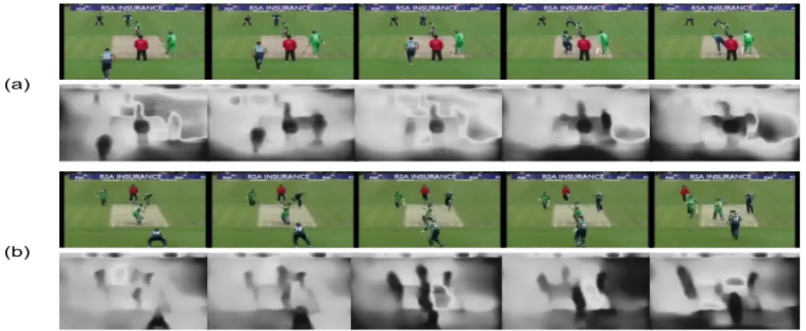
(a)

(b)

Figure 2.1: Action classes comparison: (a) “CricketBowling” and (b) “CricketShot”. Depth information about the bowler and the batters is key to telling these two classes apart. Our proposed depth2action approach exploits the depth information that is embedded in the videos to perform large-scale action recognition.

blue (RGB) domain. For instance, the “CricketShot” and “CricketBowling” classes in the UCF101 dataset [146] are often confused by the state-of-the-art models [164, 168]. This makes sense because, as shown in Fig. 2.1, these classes can be very similar with respect to static appearance, human-object interaction, and in-plane human motion patterns. Depth information about the bowler and the batters is key to telling these two classes apart.

Previous work on depth for action recognition [29, 161, 188, 166] uses depth obtained from depth sensors such as Kinect-like devices and thus is not applicable to large-scale action recognition in RGB video. We instead estimate the depth information directly from the video itself. This is a difficult problem which results in noisy depth sequences and so a major contribution of our work is how to effectively extract the subtle but informative depth cues. To our knowledge, our work is the first to perform large-scale action recognition based on depth information embedded in the video.

Our novel contributions are as follows: (i) we introducedepth2action, a novel approach for human action recognition using depth information embedded in videos. It is shown to be complementary to existing approaches which exploit spatial and translational mo-tion informamo-tion and, when combined with them, achieves state-of-the-art performance on three popular benchmarks. (ii) we propose spatio-temporal depth normalization (STDN) to enforce temporal consistency and modified depth motion maps (MDMMs) to capture the subtle temporal depth cues in noisy depth sequences. (iii) we perform a thorough in-vestigation on how best to extract and incorporate the depth cues including: image- versus

(29)

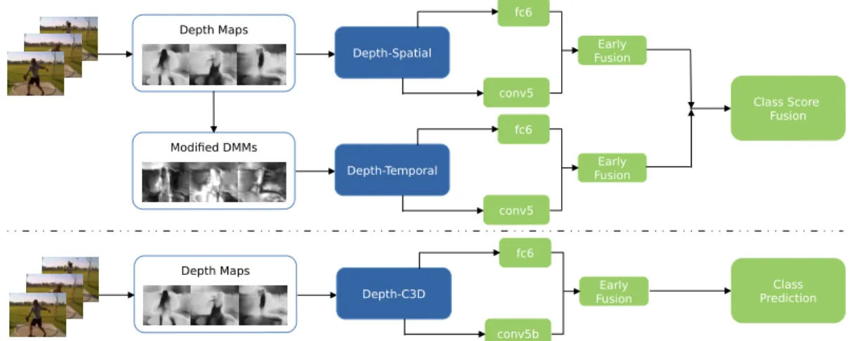
Class Score Fusion Depth Maps Modified DMMs fc6 Depth-Spatial conv5 Early Fusion fc6 Depth-Temporal conv5 Early Fusion Depth Maps fc6 Depth-C3D conv5b Early Fusion Class Prediction

Figure 2.2: Depth2Action framework. Top: Our depth two-stream model. Depth maps are estimated on a per-frame basis and input to a depth-spatial net. Modified depth motion maps (MDMMs) are derived from the depth maps and input to a depth-temporal net. Features are extracted, concatenated and input to two support vector machine (SVM) classifiers, to obtain the final prediction scores. Bottom: Our depth-C3D framework which is similar except the depth maps are input to a single depth-C3D net which jointly captures spatial and temporal depth information.

video-based depth estimation; multi-stream 2D CNNs versus 3D CNNs to jointly extract spatial and temporal depth information; CNNs as feature extractors versus end-to-end clas-sifiers; early versus late fusion of features for optimal prediction; and other design choices.

2.2 Related Work

There exists an extensive body of literature on human action recognition. We review only the most related work.

Deep CNNs: Improved dense trajectories [159] dominated the field of video analysis for several years until the two-stream CNNs architecture introduced by Simonyan and Zis-serman [144] achieved competitive results for action recognition in video. In addition, motivated by the great success of applying deep CNNs in image analysis, researchers have adapted deep architectures to the video domain either for feature representation [163, 183, 153, 197, 148] or end-to-end prediction [77, 164, 121, 176].

While our framework shares some structural similarity with these works, it is distinct and complementary in that it exploits depth for action recognition. All the works above

(30)

11

are based on appearance and translational motion in the RGB domain. We note there has been some work that exploits audio information [126]; however, not all videos come with audio and our approach is complementary to this work as well.

RGB-D Based Action Recognition: There is previous work on action recognition in RGB-D data. Chen et al. [29] use depth motion maps (DMM) for real-time human ac-tion recogniac-tion. Yang and Tian [188] cluster hypersurface normals in depth sequences to form a super normal vector (SNV) representation. Very recently, Wang et al. [166] apply weighted hierarchical DMM and deep CNNs to achieve state-of-the-art performance on sev-eral benchmarks. Our work is different from approaches that use RGB-D data in sevsev-eral key ways:

(i) Depth information source and quality: These methods use depth information ob-tained from depth sensors. Besides limiting their applicability, this results in depth se-quences that have much higher fidelity than those which can be estimated from RGB video. Our estimated depth sequences are too noisy for recognition techniques designed for depth-sensor data. Taking the difference between consecutive frames in our depth sequences only amplifies this noise making techniques such as STOP features [157], SNV representations [188], and DMM-based framework [29, 166], for example, ineffective.

(ii)Benchmark datasets: RGB-D benchmarks such as MSRAction3D [94], MSRDaily-Activity3D [162], MSRGesture3D [160], MSROnlineAction3D [194] and MSRActionPairs3D [127] are much more limited in terms of the diversity of action classes and the number of samples. Further, the videos often come with other meta data like skeleton joint positions. In con-trast, benchmarks such as UCF101 contain large numbers of action classes and the videos are less constrained. Recognition is made more difficult by the large intra-class variation.

We note that we take inspiration from [187, 166] in designing our modified DMMs. The approaches in these works use RGB-D data and are not appropriate for our problem, though, since they construct multiple depth sequences using different geometric projections, and our videos are too long and our estimated depth sequences too noisy to be characterized by a single DMM.

In summary, our depth2action framework is novel compared to previous work on action recognition. An overview of our framework can be found in Fig. 2.2.

(31)

(a)

(b)

(c)

(d)

Figure 2.3: Depth maps estimated from the video v ThrowDiscus g05 c02.avi in the UCF101 dataset. (a): raw RGB frames; (b): depth maps extracted using [98]; (c): depth maps extracted using [41]; (d): the absolute difference between consecutive depth maps in (c). Blue indicates smaller values and yellow larger ones.

2.3 Methodology

2.3.1 Depth Extraction

Since our videos do not come with associated depth information, we need to extract it directly from the RGB video data. Extracting depth maps from video has been studied for some time now [199, 147, 133]. Most approaches, however, are not applicable since they either require stereo video or additional information such as geometric priors. There are a few works [101] which extract depth maps from monocular video alone but they are computationally too expensive which does not scale to problems like ours.

We therefore turn to frame-by-frame depth extraction and enforce temporal consistency through a normalization step. Depth from images has made much progress recently [98, 9, 83, 41] and is significantly more efficient for extracting depth from video. We consider two state-of-the-art approaches to extract depth from images, [98] and [41], based on their accuracy and efficiency.

Deep Convolutional Neural Fields (DCNF) [98]: This work jointly explores the capacity of deep CNNs and continuous CRFs to estimate depth from an image. Depth is predicted through maximum a posterior (MAP) inference which has a closed-form solution. We apply the implementation kindly provided by the authors [98] but discard the time consuming “inpainting” procedure which is not important for our application. Our modified

(32)

13

implementation takes only 0.09s per frame to extract a depth map.

Multi-scale Deep Network [41]: Unlike DCNF above, this method does not utilize super-pixels and thus results in smoother depth maps. It uses a sequence of scales to pro-gressively refine the predictions and to capture image details both globally and locally. Although the model can also be used to predict surface normals and semantic labels within a common CNN architecture, we only use it to extract depth maps. Our modified imple-mentation takes only 0.01s per frame to extract a depth map.

Fig. 2.3 visually compares the per-frame depths maps generated by the two approaches. We observe that 1) [41] (Fig. 2.3c) results in smoother maps since it does not utilize super-pixels like [98] (Fig. 2.3b), and 2) [41] preserves structural details, such as the border between the sky and the trees, better than [98] due to its multi-scale refinement. Quanti-tatively, [41] also results in better action recognition performance so we use it to extract per-frame depth maps for the rest of the chapter.

2.3.2 Spatio-Temporal Depth Normalization

We now have depth sequences. While this makes our problem similar to work on action recognition from depth-sensor data such as [166], these methods are not applicable for a number of reasons. First, their inputs are point clouds which allows them to derive depth sequences from multiple perspectives for a single video as well as augment their training data through virtual camera movement. We only have a single fixed viewpoint. Second, their depth information has much higher fidelity since it was acquired with a depth sensor. Ours is prohibitively noisy to use a single 2D depth motion map to represent an entire video as is done in [166].

The first step is to reduce the noise by enforcing temporal consistency under the as-sumption that depth does not change significantly between frames. We introduce a temporal normalization scheme which constrains the furthest part of the scene to remain approxi-mately the same throughout a clip. We find this works best when applied separately to three horizontal spatial windows and so we term the method spatio-temporal depth normalization (STDN). Specifically, letxbe a frame. We then takenconsecutive frames [xt1,xt2, . . . ,xtn]

to form a volume (clip) which is divided spatially into three equal-sized subvolumes that represent the top, middle, and bottom parts [125]. We take the 95thpercentile of the depth distribution as the furthest scene element in each subvolume. The 95th percentile of the corresponding window in each frame is then linearly scaled to equal this furthest distance. We also investigated other methods to enforce temporal consistency including

(33)

intra-frame normalization, temporal averaging (uniform as well as Gaussian) with varying tem-poral window sizes, and warping. None performed as well as the proposed STDN.

2.3.3 CNNs Architecture Selection

Recent progress in action recognition based on CNNs can be attributed to two models: a two-stream approach based on 2D CNNs [144, 164] which separately models the spatial and temporal information, and 3D CNNs which jointly learn spatio-temporal features [71, 153]. These models are applied to RGB video sequences. We explore and adapt them for our depth sequences.

2D CNNs: In [144], the authors compute a spatial stream by adapting 2D CNNs from image classification [86] to action recognition. We do the same here except we use depth sequences instead of RGB video sequences. We term this ourdepth-spatial stream to distin-guish it from the standard spatial stream which we will refer to as RGB-spatial stream for clarity. Our depth-spatial stream is pre-trained on the ILSVRC-2012 dataset [139] with the VGG-16 implementation [145] and fine-tuned on our depth sequences. [144] also computes a temporal stream by applying 2D CNNs to optical flow derived from the RGB video. We could similarly compute optical flow from our depth sequences but this would be redundant (and very noisy) so we instead propose a different depth-temporal stream below in section 2.3.4.

3D CNNs: In [71, 153], the authors show that 2D CNNs “forget” the temporal information in the input signal after every convolution operation. They propose 3D CNNs which analyze sets of contiguous video frames organized as clips. We apply this approach to clips of depth sequences. We term thisdepth-C3D to distinguish it from the standard 3D CNNs which we will refer to as RGB-C3D for clarity. Our depth-C3D net is pre-trained using the Sports-1M dataset [77] and fine-tuned on our depth sequences.

2.3.4 Depth-Temporal Stream

Here, we look to augment our depth-spatial stream with a depth-temporal stream. We take inspiration from work on action recognition from depth-sensor data and adapt depth motion maps [187] to our problem. In [187], a single 2D DMM is computed for an entire sequence by thresholding the difference between consecutive depth maps to get per-frame (binary) motion energy and then summing this energy over the entire video. A 2D DMM summarizes where depth motion occurs.

(34)

15

We instead calculate the motion energy as the absolute difference between consecutive depth mapswithout thresholding in order to retain the subtle motion information embedded in our noisy depth sequences. We also accumulate the motion energy over clips instead of entire sequences since the videos in our dataset are longer and less-constrained compared to the depth-sensor sequences in [94, 127, 162, 160, 194] and so our depth sequences are too noisy to be summarized over long periods. In many cases, the background would simply dominate.

We compute one modified depth motion map (MDMM) for a clip ofN depth maps as

MDMMtstart =

tstart+N

X

tstart

|maptstart+1₋_maptstart_|_, _(2.1)

wheretstartis the first frame of the clip, N is the duration of the clip, and maptis the depth

map at framet. Multiple MDMMs are computed for each video. Each MDMM is then input to a 2D ConvNet for classification. We term this our depth-temporal stream. We combine it with our depth-spatial stream to create our depth two-stream (see Fig. 2.2). Similar to the depth-spatial stream, the depth-temporal stream is pre-trained on the ILSVRC-2012 dataset [139] with the VGG-16 network [145] and fine-tuned on the MDMMs.

We also consider a simpler temporal stream by taking the absolute difference between adjacent depth maps and inputting this difference sequence to a 2D ConvNet. We term this our baseline depth-temporal stream. Fig. 2.3d shows an example sequence of this difference. It does a good job at highlighting changes in the depth despite the noisiness of the image-based depth estimation.

2.3.5 CNNs: Feature Extraction or End-to-End Classification

The CNNs in our depth two-stream and depth-C3D models default to end-to-end clas-sifiers. We investigate whether to use them instead as feature extractors followed by SVM classifiers. This also allows us to investigate early versus late fusion. We use our depth-spatial stream for illustration.

Features are extracted from two layers of our fine-tuned CNNs. We extract the activa-tions of the first fully-connected layer (fc6) on a per-frame basis. These are then averaged over the entire video and L2-normalized to form a 4096-dim video-level descriptor. We also extract activations from the convolutional layers as they contain spatial information. We choose theconv5 layer, whose feature dimension is 7×7×512 (7 is the size of the filtered images of the convolutional layer and 512 is the number of convolutional filters). By con-sidering each convolutional filter as a latent concept, the conv5features can be converted

(35)

Table 2.1: Recognition performance of our proposed configurations on three benchmark datasets. (a): Our spatio-temporal depth normalization (STDN) indicated by (N) is shown to improve performance for all configurations on all datasets. (b): Using the CNNs to extract features is better than using them as end-to-end classifiers. Also, early fusion of features is better than late fusion of SVM probabilities. See the text for discussion on depth two-stream versus depth-C3D

(a) Effectiveness of STDN

Model UCF101 HMDB51 ActivityNet

Depth-Spatial 58.8% 37.9% 35.9% Depth-Spatial (N) 59.1% 38.3% 36.4% Depth-Temporal Baseline 61.8% 40.6% 38.2% Depth-Temporal Baseline (N) 63.3% 42.0% 39.8% Depth-Temporal 63.9% 42.6% 39.7% Depth-Temporal (N) 65.1% 43.5% 40.9% Depth Two-Stream 65.6% 44.2% 42.7% Depth Two-Stream (N) 67.0% 45.4% 44.2% Depth-C3D 61.7% 40.9% 45.9% Depth-C3D (N) 63.8% 42.8% 47.4%

(b) Features or End-to-End Classifier

Model UCF101 HMDB51 ActivityNet

Depth Two-Stream 67.0% 45.4% 44.2%

Depth Two-Streamfc6 68.2% 46.5% 45.3%

Depth Two-Streamconv5 70.1% 48.2% 47.0%

Depth Two-Stream Early 72.5% 49.7% 49.6%

Depth Two-Stream Late 70.9% 48.9% 48.7%

Depth-C3D 63.8% 42.8% 47.4%

Depth-C3Dfc6 64.9% 43.9% 47.9%

Depth-C3Dconv5b 66.7% 45.0% 49.1%

Depth-C3D Early 69.5% 46.6% 52.1%

Depth-C3D Late 67.8% 45.7% 51.0%

into 72 latent concept descriptors (LCD) [183] of dimension 512. We also adopt a spatial pyramid pooling (SPP) strategy [57] similar to [183]. We apply principle component anal-ysis (PCA) to de-correlate and reduce the dimension of the LCD features to 64 and then encode them using vectors of locally aggregated descriptors (VLAD) [70]. This is followed by intra- and L2-normalization to form a 16384-dim video-level descriptor.

Early fusion consists of concatenating the fc6 and conv5 features for input to a sin-gle multi-class linear SVM classifier [42] (see Fig. 2.2). Late fusion consists of feeding the features to two separate SVM classifiers and computing a weighted average of their probabilities. The optimal weights are selected by grid-search.

2.4 Experiments

The goal of our experiments is two-fold. First, to explore the various design options described in section 2.3 Methodology. Second, to show that our depth2action framework is complementary to standard approaches to large-scale action recognition based on appear-ance and translational motion and achieves state-of-the-art results when combined with them.

(36)

17

2.4.1 Datasets

We evaluate our approach on three widely adopted publicly-available action recognition benchmark datasets: UCF101 [146], HMDB51 [88] and ActivityNet [59]. The evaluation metric we used in this dissertation is top-1 mean accuracy (mAcc) for all three datasets. UCF101is composed of realistic action videos from YouTube. It contains 13,320 videos in 101 action classes. It is one of the most popular benchmark datasets because of its diversity in terms of actions and the presence of large variations in camera motion, object appearance and pose, object scale, viewpoint, cluttered background, illumination conditions, etc. HMDB51 is composed of 6,766 videos in 51 action classes extracted from a wide range of sources such as movies and YouTube videos. It contains both original videos as well as stabilized ones, but we only use the original videos.

Both UCF101 and HMDB51 have a standard three split evaluation protocol and we report the average recognition accuracy over the three splits.

ActivityNetAs suggested by the authors in [59], we use its release 1.2 for our experiments due to the noisy crowdsourced labels in release 1.1. The second release consists of 4,819 training, 2,383 validation, and 2,480 test videos in 100 activity classes. Though the number of videos and classes are similar to UCF101, ActivityNet is a much more challenging bench-mark because it has greater intra-class variance and consists of longer, untrimmed videos. We use both the training and validation sets for model training and report the performance on the test set.

2.4.2 Implementation Details

We use the Caffe toolbox [72] to implement the CNNs. The network weights are learned using mini-batch stochastic gradient descent (256 frames for two-stream CNNs and 30 clips for 3D CNNs) with momentum (set to 0.9).

Depth Two-Stream: We adapt the VGG-16 architecture [145] and use ImageNet models as the initialization for both the depth-spatial and depth-temporal net training. As in [164], we adopt data augmentation techniques such as corner cropping, multi-scale cropping, horizontal flipping, etc. to help prevent overfitting, as well as high dropout ratios (0.9 and 0.8 for the fully connected layers). The input to the depth-spatial net is the per-frame depth maps, while the input to the depth-temporal net is either the depth difference between adjacent frames (in the baseline case) or the MDMMs. For generating the MDMMs, we set

(37)

decreases from 0.001 to 1/10 of its value every 15K iterations, and the training stops after 66K iterations. For the depth-temporal net, the learning rate starts at 0.005, decreases to 1/10 of its value every 20K iterations, and the training stops after 100K iterations.

Depth-C3D:we adopt the same architecture as in [153]. The Depth-C3D net is pre-trained on the Sports-1M dataset [77] and tuned on estimated depth sequences. During fine-tuning, the learning rate is initialized to 0.005, decreased to 1/10 of its value every 8K iterations, and the training stops after 34K iterations. Dropout is applied with a ratio of 0.5.

Note that since the number of training videos in the HMDB51 dataset is relatively small, we use CNNs fine-tuned on UCF101, except for the last layer, as the initialization (for both 2D and 3D CNNs). The fine-tuning stage starts with a learning rate of 10−5 and converges in one epoch.

2.4.3 Results

Effectiveness of STDN: Table 2.1(a) shows the performance gains due to our proposed normalization. STDN improves recognition performance for all approaches on all datasets. The gain is typically around 1-2%. We set the normalization window (n in section 2.3.2) to 16 frames for UCF101 and ActivityNet, and 8 frames for HMDB51. We further observe that (i) Depth-C3D benefits from STDN more than depth two-stream. This is possibly because the input to depth-C3D is a 3D volume of depth sequences while the input to depth two-stream is the individual depth maps. Temporal consistency is important for the 3D volume. (ii) Depth-temporal benefits from STDN more than depth-spatial. This is expected since the goal of the normalization is to improve the temporal consistency of the depth sequences and only the depth-temporal stream “sees” multiple depth-maps at a time. From now on, all results are based on depth sequences that have been normalized.

Depth Two-Stream versus Depth-C3D: As shown in Table 2.1(a), depth two-stream performs better than depth-C3D for UCF101 and HMDB51, while the opposite is true for ActivityNet. This suggests that depth-C3D may be more suitable for large-scale video analysis. Though the second release of ActivityNet has a similar number of action clips as UCF101, in general, the video duration is much (30 times) longer than that of UCF101. Similar results for 3D CNNs versus 2D CNNs was observed in [100]. The computational efficiency of depth-C3D also makes it more suitable for large-scale analysis. Although our depth-temporal net is much faster than the RGB-temporal net (which requires costly optical flow computation), depth-two stream is still significantly slower than depth-C3D.

(38)

19

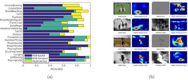
(a)

RGB Frame RGB-Spatial-conv5 Optical Flow RGB-Temporal-conv5

Depth Map Depth-Spatial-conv5 Modified DMM Depth-Temporal-conv5

RGB Frame RGB-Spatial-conv5 Optical Flow RGB-Temporal-conv5

Depth Map Depth-Spatial-conv5 Modified DMM Depth-Temporal-conv5

(b)

Figure 2.4: (a) Recognition results on the first split of UCF101. Plot showing the classes for which our proposed depth2action framework (yellow) outperforms RGB-spatial (blue) and RGB-temporal (green) streams. (b) Visualizing the convolutional feature maps of four models: RGB-spatial, RGB-temporal, depth-spatial, and depth-temporal. Pairs of inputs and resulting feature maps are shown for each model for two actions, “CriketBowling” and “ThrowDiscus”.

We therefore recommend using depth-C3D for large-scale applications.

CNNs for Feature Extraction versus End-to-End Classification: Table 2.1(b) shows that treating the CNNs as feature extractors performs significantly better than using them for end-to-end classification. This agrees with the observations of others [12, 153, 203]. We further observe that the VLAD encoded conv5features perform better than fc6. This improvement is likely due to the additional discriminative power provided by the spatial information embedded in the convolutional layers. Another attractive property of using feature representations is that we can manipulate them in various ways to further improve the performance. For instance, we can employ different (i) encoding methods: Fisher vector [125], VideoDarwin [44]; (ii) normalization techniques: rank normalization [91]; and (iii) pooling methods: line pooling [203], trajectory pooling [163, 203], etc.

Early versus Late Fusion: Table 2.1(b) also shows that early fusion of features through concatenation performs better than late fusion of SVM probabilities. Late fusion not only results in a performance drop of around 1.0% but also requires a more complex processing pipeline since multiple SVM classifiers need to be trained. UCF101 benefits from early fusion more than the other two datasets. This might be due to the fact that UCF101 is a trimmed video dataset and so the content of individual videos varies less than in the other

(39)

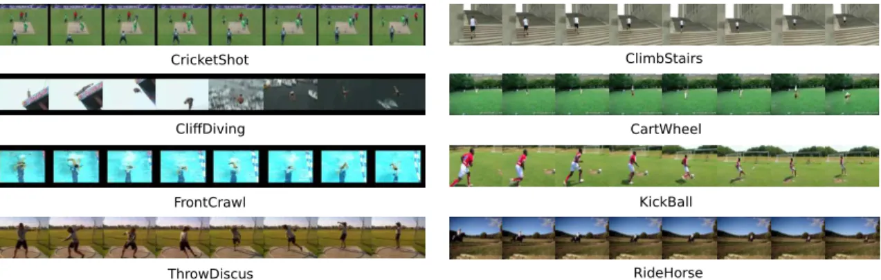
CliffDiving FrontCrawl ThrowDiscus CricketShot ClimbStairs CartWheel KickBall RideHorse

Figure 2.5: Sample video frames of action classes that benefit from depth information. Left: UCF101. Right: HMDB51.

two datasets. Early fusion of multiple layers’ activations is typically more robust to noisy data.

Depth2Action: We thus settle on our proposed depth2action framework. For medium-scale video datasets like UCF101 and HMDB51, we perform early fusion of conv5and fc6 features extracted using a depth two-stream configuration. For large-scale video datasets like ActivityNet, we perform early fusion of conv5b and fc6 features extracted using a depth-C3D configuration. These two models are shown in Fig. 2.2.

2.4.4 Discussion

Class-Specific Results: We investigate the specific classes for which depth information is important. To do this, we compare the per-class performance of our depth2action framework with standard methods that use appearance and translational motion in the RGB domain. We first compute the performances of an RGB-spatial stream which takes the RGB video frames as input and an RGB-temporal stream which takes optical flow (computed in the RGB domain) as input. We then identify the classes for which our depth2action performs better than both the RGB-spatial and RGB-temporal streams. We compute these results for the first split of the UCF101 dataset. Fig. 2.4a shows the 20 classes for which our depth2action framework performs best (in order of decreasing improvement). For example, for the class CricketShot, RGB-spatial achieves an accuracy of around 0.18, RGB-temporal achieves around 0.62, while our depth2action achieves around 0.88. (For those classes where RGB-spatial performs better than RGB-temporal, we simply do not show the performance of RGB-temporal.) Depth2action clearly represents a complementary approach especially for classes where the RGB-spatial and RGB-temporal streams perform relatively poorly